Università degli Studi “Roma Tre”
Dipartimento di Economia
Scuola Dottorale in Economia e Metodi Quantitativi
Dottorato in Economia dell’Ambiente e dello Sviluppo
XXVII ciclo
Energy substitution by sector: technological flexibility
and the impact of mitigation policy
Elena Paglialunga
Supervisor: Prof.ssa Valeria Costantini
Co-Supervisors: Dott. Alessandro Antimiani, Prof. Simone Borghesi, Prof. Francesco Crespi
Coordinatore: Prof. Luca Salvatici
Table of content
Introduction
9
Elasticity of substitution in capital-energy relationship: a sector-based panel
estimation approach
1. Introduction 13
2. Elasticity of substitution between capital and energy: relevance and interpretation 16
3. Literature review 19
3.1 Early studies: substitution or complementarity between energy and capital 19 3.2 Energy and economic output: from Granger causality to Fully Modified OLS 21 3.3 Measuring the elasticity of substitution between energy and capital at sector level 24
4. Empirical analysis 30
4.0 Empirical strategy 30
4.1 Dataset analysis 32
4.2 Long run relationships between energy and economic dimensions at sector level 35 4.3 Translog production function and Allen Elasticity of Substitution 39
5. Empirical results 42
5.1 Results of stationarity and cointegration analysis 42
5.2 Capital-energy Allen Elasticity of Substitution 46
6. Conclusion 51
References 53
Appendix 57
A sensitivity analysis of a dynamic climate-economy CGE model (GDynE) to
empirically estimated energy-related elasticity parameters
1. Introduction 59
2. Literature Review 60
3. Model 64
3.1 Model description 64
3.2 Alternative sets of elasticity of substitution parameters 65
3.3 Baseline and policy scenarios 66
4. Results 70
4.1 Comparison between standard and empirically-based elasticity parameters
4.2 Comparison in model results between economy-wide and sector-specific elasticity
parameters 80
5. Conclusion 86
References 88
Appendix 90
EU climate policy up to 2030: reasoning around timing, overlapping instruments
and cost effectiveness
1. Introduction 99
2. Literature Review 101
3. Model 106
3.1 Model improvements 108
3.2 Baseline and policy scenarios 111
4. Results 114
4.1 Comparison between policy scenarios with and without RD investment in green
technologies 114
4.2 Comparison between alternative timing of emission reduction targets 121
5. Conclusions 127
References 129
Appendix 132
List of tables and figures
Elasticity of substitution in capital-energy relationship: a sector-based panel
estimation approach
Table 1 - Early empirical studies on capital-energy substitution and complementarity 20
Table 2 - Summary of literature review on disaggregated sectors 23
Table 3 - Review of aggregate capital-energy elasticity of substitution estimates 27 Table 4 - Review of sector capital-energy elasticity of substitution for manufacturing
industries 30
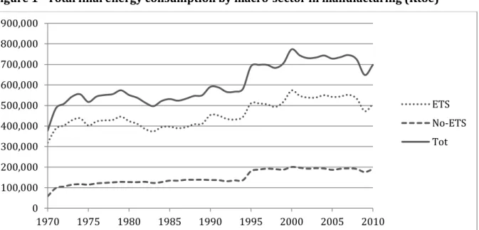
Figure 1 - Total final energy consumption by macro-sector in manufacturing (Ktoe) 35 Figure 2 - Distribution of factors and output share by sector (average on 1975-2008) 35
Table 5 - Unit root tests 42
Table 6 - Pedroni Panel Cointegration Test 43
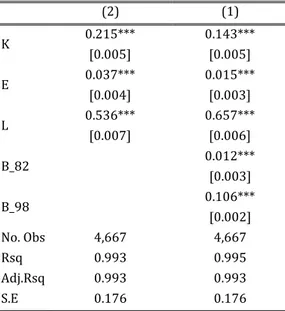
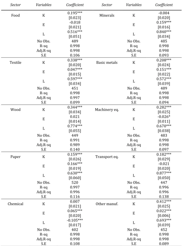
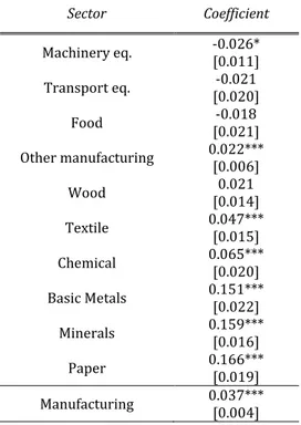
Table 7 - Long-run elasticities from panel FMOLS for whole industry (1975-2008) 43 Table 8 - Long-run elasticities from panel FMOLS for sub-sectors (1975-2008) 45 Table 9 – Energy long-run elasticities from panel FMOLS for sub-sectors (1975-2008) 46 Table 10 - Translog estimation for aggregate manufacturing industry and sub-sectors
in FMOLS (1975-2008) 47
Table 11 – KE-AES by manufacturing sector 50
Appendix
Table A.1 - Energy intensity by manufacturing sector 57
Table A.2 - Capital intensity by manufacturing sector 57
Table A.3 – KE-AES by manufacturing sector (1990-1994) 58
Table A.4 – KE-AES by manufacturing sector (1995-1999) 58
Table A.5 – KE-AES by manufacturing sector (2000-2004) 58
Table A.6 – KE-AES by manufacturing sector (2005-2008) 58
A sensitivity analysis of a dynamic climate-economy CGE model (GDynE) to
empirically estimated energy-related elasticity parameters
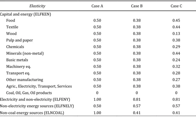
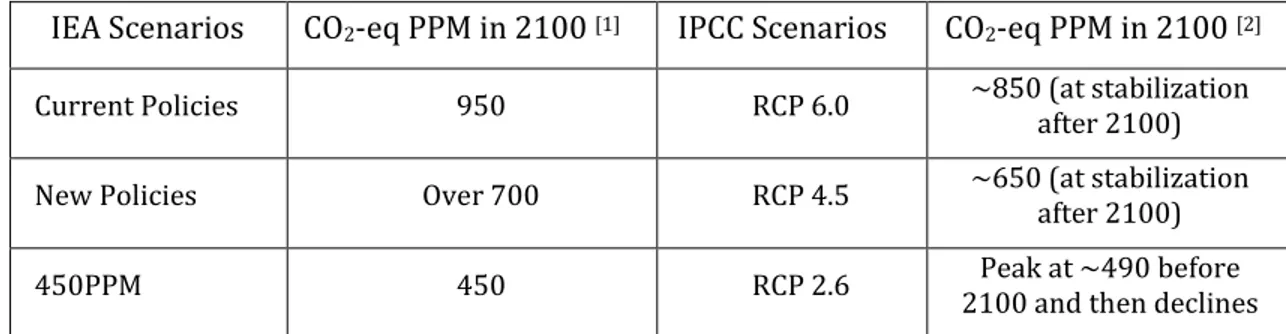
Table 1 - Values of alternative substitution elasticities in energy-related nests 66 Table 2 - Relation between IEA and IPCC Scenarios based on CO2-eq PPM 67
Figure 1 - CO2 trends in 450PPM and BAU, Case A vs. Case B 71
Table 3 – Comparison between Cases A, A1 and B applied to CTAX 72
Table 4 - Carbon tax level and permit price in 450PPM, Case A vs. Case B (USD/ton CO2) 73 Figure 2 – Marginal Abatement Cost curves at the world level in IET scenario,
Case A vs. Case B 74
Table 6 – Comparison in allocative efficiency and EV, Case A vs. Case B (Bln USD) 76 Table 7 - Differences in GDP between Case A and Case B in IET scenario (Mln USD) 77 Figure 3 – Differences in GDP between IET and BAU, Case A vs. Case B (Bln USD) 77 Figure 4 - Differences in Annex I GDP between IET and BAU, Case A vs. Case B (Bln USD) 78 Table 8 – Changes in fuel mix between 2010 and 2050 (Case A vs. Case B) 79 Table 9 – Differences in fuel mix shares between IET and BAU, Case A vs. Case B 79 Table 10 – Differences in carbon intensity w.r.t. changes in σKE, Case C vs. Case B 82 Figure 5 – Differences in output in BAU for Annex I countries, Case C vs. Case B 83 Figure 6 – Differences in output in BAU for non-Annex I countries, Case C vs. Case B 83 Table 11 – Differences in price changes in BAU, Case C vs. Case B (2050) 84 Figure 7 – Differences in output in IET (cumulated 2010-2050), Case C vs. Case B 84 Figure 8 – Differences in export flows in IET (cumulated 2010-2050), Case C vs. Case B 85
Figure 9 – Marginal Abatement Cost curves (Par. C) 85
Appendix
Table A.1 - List of GDYnE countries 90
Table A.2 - List of GDYnE commodities and aggregates 91
Table A.3 - List of GDYnE Regions 92
Table A.4 - List of GDYnE aggregates 92
Table A.5 - Baseline GDP Projections to 2050 (Bln constant USD) 93
Table A.6 - Baseline CO2 Projections to 2050 (Gt CO2) 94
Table A.7 – Differences in GDP between IET and CTAX Scenarios, Case A vs. Case B
(Mln USD) 94
Table A.8 - Differences in fuels mix in IET w.r.t. BAU, Case A vs. Case B (%) 95
Table A.9 – Carbon intensity (Ton/Mln USD, *10,000) 96
Table A.10 – Differences in output between IET scenarios, Case C vs. Case B (%) 97
EU climate policy up to 2030: reasoning around timing, overlapping instruments
and cost effectiveness
Table 1 - Carbon Tax level for EU27 (US Dollars per ton) 115
Table 2 - EU Carbon Tax Revenue for EU27 (Mln US Dollars) 115
Table 3 – Annual flows of public investment in RD activities for EU27 (Mln US Dollars) 116
Table 4 – GDP losses with respect to BAU for EU27 (%) 117
Table 5 - EV losses with respect to BAU for EU27 (%) 117
Figure 1 - Differences in Allocative Efficiency w.r.t. 450PPM for EU27 (Mln US Dollars) 117 Figure 2 – Changes in export flows in 450PPM scenarios w.r.t. BAU for EU27 (%) 119
Table 6 – Changes in electricity prices in EU27 (%) 119
Table 7 - Energy Intensity for EU27 (Toe/Mln US Dollars) 121
Figure 4 - CO2 emission paths for EU27 (Mtoe) 122
Figure 5 – GDP level for EU27 (Mln US Dollar) 122
Figure 6 – Changes in export flows in 450PPM w.r.t. BAU for EU27 (%) 123 Figure 7 – Changes in export flows in EU2030 w.r.t. BAU for EU27 (%) 123
Table 8 – Comparison between EU2030 and 450PPM scenarios 124
Figure 8 - Carbon Tax level for EU27 (US Dollars per ton) 124
Figure 9 - Marginal abatement cost curves for EU27 125
Table 9 – Comparison between EU2030-10%, 450PPM-10% and 450PPM-20% scenarios 126 Appendix
Table A.1 - List of GDYnE countries 132
Table A.2 - List of GDYnE commodities and aggregates 133
Table A.3 - List of GDYnE Regions 134
Table A.4 - List of GDYnE aggregates 134
Table A.5 - Baseline GDP Projections to 2050 (Bln constant USD) 135
Table A.6 - Baseline CO2 Projections to 2050 (Gt CO2) 136
Table A.7 - Changes in output value from BAU for EU27 (%) 137
Table A.8 - Changes in export value from BAU for EU27 (%) 138
Figure A.1 - Changes in export flows in 450PPM scenario w.r.t. BAU for ROW (%) 139 Figure A.2 - Changes in export flows in 450PPM scenario w.r.t. BAU for ROW (%) 139 Figure A.3 - Changes in export flows in 450PPM scenario w.r.t. BAU for ROW (%) 139
Introduction
The impact of climate mitigation policies on economic activity is a longstanding controversial issue justifying the large strand of literature analysing the effect of climate change policies in terms of environmental and economic costs, also in light of the numerous international agreements and negotiations. Starting with the constitution of the Intergovernmental Panel on Climate Change (IPCC), through the 1992 United Nations Framework Convention on Climate Change (UNFCCC), the international community has ratified the Kyoto Protocol (KP) assigning greenhouse gas (GHG) reduction targets for Annex I countries compared to 1990 levels. From then to the current climate policy agenda approved by the European Union in October 2014, mitigation of climate change still constitutes a challenging long term objective at the global level, and it is particularly relevant for the European Union.
These concerns justify the interests in the assessment of climate change impacts given that mitigation costs are an essential input to policy decisions. One of the driving criteria of the KP is explicitly directed toward a minimisation of the overall costs associated with emission reduction and, given both the global scale of the problem and the differences in marginal abatement costs, the KP allows domestic emission reduction efforts to be complemented by various flexible mechanisms, including permit trading. To this purpose, the sole existing permit market under the KP umbrella is the European Union Emission Trading Scheme (EU ETS), started in 2005 as a core instrument within the overall EU climate strategy.
Moreover, given the global scope of environmental policies in an open economy and considering environmental quality as global public good (as the controversial international Post-Kyoto negotiations on reduction targets prove), a second aspect to carefully account for is the regional distribution of those costs. In addition, changes in relative energy costs across countries not only influence industrial and energy competitiveness but also economic competitiveness, and energy-intensive sectors are more and primarily affected by increases in energy prices.
In this context, it is not surprising the comprehensive use of applied models representing the global economy, the relations between the economic, social and technological dimension, across countries and the economic sectors. Models may differ in purpose and perspective, depending on the short or long-term time horizon, focussing on a single country or globally, analysing unilateral or coordinated measures. Recently, great efforts have been directed to link bottom-up technology models into partial or general equilibrium models to provide a better representation of the key energy system in more details.
In this light, the current work is structured in three main parts. The first is an analysis of the energy substitutability in the context of capital-energy relationship, centred on a sector-based panel estimation approach. Several types of impact forecasting tools for the assessment of economic impacts of climate actions have been developed based on top-down, bottom-up or integrated approaches. In particular, Computable General Equilibrium (CGE) models, which have been extensively employed to analyse policy incidence and forecast economic impacts of climate actions, are extremely sensitive to exogenous assumptions on such energy-related elasticity parameters. Indeed, one specific issue under investigation is the role of behavioural parameters in influencing climate models’ results. This part of the work specifically addresses the computation of capital-energy substitution elasticity values in ten manufacturing sectors for OECD countries considering different time horizon and aggregation level. Firstly, the long run elasticities are estimated at aggregate level for the whole manufacturing sector as well as for single sectors during the time span between 1970 and 2008 for a panel of 21 OECD countries with a panel cointegration technique. We then focus on the elasticity of substitution between capital and energy, at the aggregate manufacturing level (1970-2008), distinguishing ten manufacturing sectors (between 1990 and 2008, and for separate sub-periods), and comparing several alternative econometric estimation methods. These results can inform climate-economic models in order to assess more precisely the reaction of the climate-economic system to the implementation of climate policies, in terms of both overall abatement costs and their distribution across different sectors.
The second part presents a sensitivity analysis of a dynamic climate-economy CGE model (GDynE), where we specifically focus on testing the effect of changing the values for the elasticity parameters. In fact, Computable General Equilibrium (CGE) models are especially suitable to analyse the effect of carbon-abating policies considering they can capture the linkages between regulated and non-abating countries in terms of competitiveness through trade channel, but also through investment dynamics in the long run. However, these models need be improved and validated with detailed information on technological and energy modules in order to produce more reliable results. As far as CGE models are concerned, this kind of information is represented by elasticities, or behavioural parameters, which regulate the
substitution processes in response to changes in relative prices. Those behavioural parameters represent a component of the technology information and regulate how the model responds to exogenous policy shock, and, in particular, the elasticity of substitution between energy and capital is a measure of technological flexibility related to energy use. Thus, we shall conduct a sensitivity analysis considering three different sets of elasticity parameters: the standard GTAP version; the parameters derived from Koetse et al. (2008) on energy-capital elasticity of substitution and from the meta analysis by Stern (2012) on interfuel-substitution; and the sector-specific KE elasticity parameters econometrically estimated in the previous part.
Finally, in the third part the focus is on the climate policy strategy of the European Union to 2030 that was discussed in October 2014. This so called EU2030, as the previous strategy EU2020, combines several tools and different objectives, and the assessment of the mitigation costs needs also to consider the potential trade-offs or complementarities among simultaneous policies. This framework defines three goals to be achieved by 2030: a 40% GHG reduction with respect to 1990 levels, the EU target of at least 27% for the share of renewable energy and a 27% increase in energy efficiency. The main instrument to reduce GHG emissions is the European Emission Trading System (EU ETS), which covers the energy and industry sectors. The renewable energy goal does not set binding national targets and leaves each Member States free to choose which types of supporting framework to implement (e.g., feed-in tariff and premium, green certificates or quota system). Hence, in the light of the recent debate around the effectiveness and the optimality of complex policy mix, especially in the case of environmental and innovation public support, the EU approach to climate change represents an interesting case study to be investigated, both in term of complementarity among policy measures and timing of the abatement targets. This last part of the work relies on a simple theoretical approach and on the GDynE, the dynamic CGE climate-economic model considered in the previous part. The aim is to suggest some reflections upon potential trade-offs or complementarity among different policy instruments within a complex climate policy mix, with particular attention to the mechanisms behind prevailing effects in terms of cost effectiveness, economic competitiveness and optimal taxation.
Elasticity of substitution in capital-energy
relationship: a sector-based panel estimation
approach
1. Introduction
Climate change mitigation policies promote the abatement of greenhouse gases (GHG) through the reduction of energy consumption from fossil fuels, the production of renewable energy and the diffusion of low carbon technologies. Starting with the constitution of the Intergovernmental Panel on Climate Change (IPCC), through the 1992 United Nations Framework Convention on Climate Change (UNFCCC), the international community has ratified the Kyoto Protocol (KP) assigning GHG reduction targets for Annex I countries compared with 1990 levels. One of the driving criteria of the KP is explicitly directed toward a minimisation of the overall costs associated with emission reduction and, given both the global scale of the problem and differences in marginal abatement costs, the KP allows domestic emission reduction efforts to be complemented by various flexible mechanisms, including permit trading. To this purpose, the sole existing permit market under the KP umbrella is the European Union Emission Trading Scheme (EU ETS), started in 2005 as a core instrument within the overall EU climate strategy.
In this context, increased interest in analysing the role that energy plays in production processes is more than justified given that the potential impacts, in economic and environmental terms, of climate policies are strongly influenced by several factors. Few examples are the specific energy mix, the energy intensity of the production process, energy prices and responses by the markets, together with the technological opportunities to be
exploited when facing binding constraints in energy consumption.
According to the IEA (2013), the impact of changes in energy prices (especially considering the existence of regional disparities) on economic and industrial competitiveness has been addressed since higher the share of energy cost on total production costs, more vulnerable the economic activity is to changes in energy prices. At the same time, more an economy is based on energy intensive activities, and more severe the consequences of an increase in energy prices can be.
In addition, even considering the possibility of technological advancements that can make production processes more energy efficient, concerns about the possible negative impacts of climate policies still rise, in terms of firm profitability and distribution across sectors of the associated costs.
Given the characteristics of supply and demand for energy and the relevance of the distribution of the policy impacts, the analysis of climate change policies has been largely done using energy economic modelling and literature in this regard is longstanding. Impact forecasting assessment tools are based on both top-down or bottom-up approaches, or are integrated as Integrated Assessment Models (IAMs). Whatever modelling approach is chosen, the specific energy-related behavioural parameters are crucial in influencing results. In particular, Computable General Equilibrium (CGE) models have been extensively employed to analyse policy incidence and forecast economic impacts (see Antimiani et al., 2013a for a review).
Results in the assessment exercise for abatement costs with respect to the role played by the energy mix, energy prices and technological opportunities are all influenced by behavioural parameters that, in applied models, are exogenously given most of the time. In this sense, the criticism to these models is due to the fact that the results can be highly dependent on the value of the behavioural parameters (or elasticities), which are not always validated enough (Okagawa and Ban, 2008). In other words, as Böhringer (1998) has pointed out, these models need to be improved with the inclusion of more detailed technological information that is indeed represented by elasticity parameters.
In particular, the economic impact of abatement policies is strongly sensitive to the values assigned to the elasticity of substitution between capital and energy in the industrial sector (Antimiani et al., 2013b; Nijkamp et al., 2005). Concerns arise mainly when the inter-sector distribution of abatement costs is under scrutiny, since energy-intensive sectors will face more challenging efforts to be compliant (Borghesi, 2011; Hoel, 1996; OECD, 2003, 2005). The strong heterogeneity of the reaction of different industrial sectors to the same abatement policy produces uncertainty about the distributive effects, thus reducing the potential role of CGE models in supporting policy design. This is, for instance, a major alarm in the assessment of the
potential impact of the EU ETS on the competitiveness performance of energy intensive industries, as emphasized in the growing debate on potential carbon leakage and trade policy reactions (Kuik and Hofkes, 2010).
To increase the reliability of the model and its results, the introduction of econometric estimated values for the parameter in the model, driven from historical data, is a first step to ensure that the model will not incorrectly represent the effect of exogenous shocks (and the policy conclusions driven by the results).
Furthermore, the introduction of sector specific parameters is especially relevant for the improvement in the assessment of abatement costs and, above all, sector-based capital-energy elasticity values are key factors when alternative mitigation policies are under scrutiny. In fact, energy-intensive and capital-intensive sectors are characterised by different input shares and different degree of technological content and this imply differences in potentials and cost effectiveness in the responses to energy reduction policies among industries.
In this respect, the debate is still open on whether or not (and if so in which measure) the introduction of climate change policies could have a detrimental effect on competitiveness and economic performances, where particular regard is focused on energy-intensive industries. Moreover, it has also to be noted that the relative importance of the different sectors can vary substantially across countries and regions, in term of both economic value added and employment, and this regional differentiation will also benefits from a more detailed sectoral representation.
The uncertainty given by behavioural exogenous parameters used in forecasting models mainly derives from the absence of a consensus on empirical estimations, or by the scarce availability of punctual estimated values. To this end, the purpose of this work is to partially fill this gap by proposing an empirical framework able to reduce uncertainty in the estimation of elasticity of substitution parameters in capital-energy relationships.
More specifically, the novelties of the work with respect to the existing literature are: i) energy-output elasticities are computed for disaggregated manufacturing sectors for a long time span (1970-2008) for a panel of 21 OECD countries; ii) capital-energy substitution elasticity is estimated at aggregate level for the whole manufacturing sector for the same panel of countries; iii) substitution elasticities are also accurately estimated for 10 distinguished manufacturing sectors for the same time span and panel of countries; iv) average substitution values at sector level are computed by comparing several alternative econometric estimation methods; v) average substitution values at sector level are also computed for separate sub-periods in order to trace the dynamics over time of these behavioural parameters.
The rest of the work is structured as follows. Section 2 provides a detailed literature review on how the concept of elasticity of substitution between capital and energy has evolved in the
last decades. Section 3 gives a description of different methodological approaches used for empirical estimation, Section 4 describes the methodology adopted in this paper for empirical estimation, Section 5 contains empirical results and Section 6 concludes the paper.
2. Elasticity of substitution between capital and energy: relevance and interpretation Understanding the substitution possibilities between energy (E) and capital (K), as well as those between different fuels such as renewables, fossil fuels and electricity, has been a longstanding issue of interest in energy economics literature. In fact, considering a production side approach, “the adoption of energy-saving technologies can be represented by substitution of capital for energy” (Koetse et al., 2008, p. 2237) and the elasticity of substitution between E and K is crucial for policies aimed at reducing energy consumption and the concentration of polluting emissions.
It is not surprising if a large strand of literature is trying to assess the magnitude of these substitution possibilities. Bounds on energy supply, rising energy prices and emission reduction targets can induce changes in the composition of input and energy mix and the impact of these changes strongly depends on the undergoing level of substitutability.
The elasticity of substitution can be defined as the reaction of an economic system to substitute one input with another where the higher the magnitude is (the absolute value assumed by the elasticity parameter), then the stronger the changing effect will be, whereas the positive or negative sign is used to distinguish between substitution or complementarity. This behavioural parameter reflects the role that an input plays in production processes by considering how it is combined with the others. Considering the specific context of interest of this work, it gives information on the scope for new intervention to reduce energy consumption, and, to some extent, represents the overall (production) conditions influencing how difficult or costly it is to reduce energy consumption through the introduction of new capital (e.g., new and less energy requiring machinery), or any other investment able to modify the production process.
Given a certain target for emission reduction, if the elasticity between E and K is low, then the costs for being compliant will be higher. As Golub (2013) points out, the elasticity of substitution between E and K basically measures the degree of technological flexibility: the lower the level then, ceteris paribus, the higher will be the reduction in output required to achieve the established target for cutting emissions. This is an energy-related level of technological flexibility that, together with capital accumulation, rate of technical progress and changes in the sectoral composition of output, describes the technology in CGE models.
Early research questions were mainly focused on investigating the nature itself of the relationship between K and E and whether it indicates complementarity or substitutability. The nature of the relationship is quite crucial in assessing the impact of alternative policy design. If the inputs are complement, they will respond to price changes moving in the same direction, thus promoting innovation and diffusion of less energy-requiring technologies will be more appropriate instruments to reduce energy consumption. On the other hand, if they are substitute, as a consequence of a change in relative prices, the share of energy will be reduced but the level of capital will increase, and a carbon tax could be less harmful than the former case (Tovar and Iglesias, 2013).
In the same line of reasoning, while complementarity and substitutability should be ascribed to a short run view, a parallel strand of literature has also investigated the nature of causal relation between energy and economic output in the long run. Besides the impact it has if combined with capital, energy also has a direct contribution on output and energy-output elasticity has therefore been largely investigated, both in CGE literature and in terms of causality relationships. In this second case, starting from an analysis of the causal direction, the magnitude, sign and significance of these parameters have also been investigated (Ortuz, 2010). Also in this case, by implementing sector-specific estimations, the reliability of parameter values will improve substantially (Costantini and Martini, 2010). Nonetheless, the level of disaggregation for sector-based analyses is not deep since only macro sectors (e.g., residential, commercial, industry) have been used for long run causality estimations.
Later contributions on capital-energy substitution elasticity moved from the issue of complementarity/substitutability to refining the econometric design in order to obtain more realistic estimations to be used in energy forecasting models. In these models, the elasticity parameters measure how sensitive economic agents are to price changes (as for instance how responsive the demand for a good is with respect to changes in relative prices or income) and determine the size of the demand adjustments. It is a crucial parameter in many energy-related models because it is a means through which changes in energy prices affect, differently according to magnitude, the supply and demand for energy, the level of capital investment and output, and the distribution of the associated costs among different sectors and countries. Thus, econometric evaluations from historical data will increase the reliability of the model results because if the parameter values are misspecified, the model will incorrectly represent the effect of exogenous shocks and policy conclusions will not be reliable (Beckam et al., 2011).
While at the general level elasticities of substitution are crucial parameters influencing the results induced by policy shocks, in selected forecasting models, and specifically in CGE models, the computation method may not support complementarity conditions (Böhringer, 1998). This is the main explanation for increasing interest in econometric estimations of the substitution
between energy and capital imposing restrictions in order to obtain a positive estimated value. Several examples available in the international scientific literature reveal the crucial role of elasticity of substitution between K and E. Just to quote a few, Jacoby et al. (2004) analyse the effect of technological change in reducing GHG emissions and find that capital-energy substitution elasticity is the key parameter in the MIT EPPA model given that changes in its magnitude determine large variations in costs associated to a “Kyoto forever” scenario for USA. Antimiani et al. (2013b) and Burniaux and Martin (2012) study the impact on carbon leakage assessment and their results show that when elasticities are higher, the level of carbon leakage is also higher. The relevance of the elasticity has also been studied in rebound effect literature, as can be seen in the works of Saunders (2000, 2008) and the review from Broadstock et al. (2007). Okagawa and Ban (2008) estimate the substitution elasticities between energy and capital at the sector level for a panel of OECD countries and their results show that, compared with the new parameter scenario, in the former specification the carbon price required to reach the objective is overestimated by 44% (and the distribution of the reduction efforts is also different). Lecca et al. (2011) analyse the impact of different separability assumptions among inputs on elasticity values and CGE model results. They therefore conclude that the inclusion of energy in different nesting structures produces significant differences in the estimation results and that capital-energy elasticity, in particular, determines a large variation in energy use, economic growth and other macroeconomic indicators.
Most of these models, however, assume the same values for these parameters in all sectors and regions since empirical estimations for deeper disaggregation at sector level are not reliable.
Hence, the reliability of impact assessment of abatement costs will largely benefit from the implementation of model settings with sector-based capital-energy elasticity values. The reasons behind this requirement can be synthesized as follows. First, the assumption of equal values for energy-intensive and capital-intensive sectors means that the reaction capacity of these sectors will be the same with respect to energy reduction policies whereas the cost shares for single inputs will be substantially different. Second, it is implicitly assumed that the degree of technological content of the production function is equal whereas the capacity of energy-intensive sectors to rapidly reduce their own energy content is rather lower than for other industries.
These features are at the basis of fears regarding the reduction in competitive performance of energy-intensive industries which is misunderstood if equal elasticity values are included in model settings. More importantly, given the different economic structures across regions, a more detailed sectoral representation will also result in a more accurate regional differentiation in terms of the distribution of abatement costs.
3. Literature review
3.1. Early studies: substitution or complementarity between energy and capital
Early studies investigating the linkages between non-energy inputs, technology structure and economic output in terms of energy substitutability took advantage of the works on flexible possibility frontiers, which made the substitution possibilities between production factors the aim of further econometric studies. The Trascendental Logarithmic Function (or Translog) from Christensen et al. (1973, 1975), in particular, has been one of the most popular because setting only a few constraints on the input-output relationship allows for unrestricted elasticities.
Bernd and Wood (1975) analysed industrial demand for energy focusing on the cross-substitution between energy and non-energy inputs in the US manufacturing industry during the period 1947-1971. They used the time series data to test a Translog cost function with four inputs (capital, labour, energy and materials, i.e. the KLEM model) and the results showed energy and capital to be strong complement (negative elasticity of substitution ranging from -3.2 to -1.4). In this case, an increase in energy prices can have a negative impact not only on the demand for energy but also on capital investments, making structural adjustments more difficult.
On the other hand, Griffin and Gregory (1976), using the same methodology on a KLE model, studied the manufacturing sector in nine industrialised countries (in the period 1955-1969)1 focusing on the cross section variation and using a sample of four benchmark years. In this case, the elasticities were always positive (around 1), implying substitutability between capital and energy. Following this line of research, many other studies tried to assess the elasticity of substitution (or complementarity) between energy and capital, e.g. Hudson and Jorgenson (1974), Pindyck (1979), Hunt (1984), Thompson and Taylor (1995), Nguyen and Streitweiser (1997) (see Table 1). Although there are a large number of empirical estimates, no unanimous conclusion has been reached yet, both in terms of sign and magnitude (Apostolakis, 1990; Thompson, 2006).
Two main differences between these works were the central issues of the initial debate, and these are the use of time series or cross section data and a KLEM instead of a KLE model. Cross section studies, capturing long run factor adjustments, usually found that capital and energy were substitutes whereas time series cases typically represented the (short run) complementarity between them. Time series data reflect dynamic adjustments to technical changes and external shocks whereas cross section data capture structural differences between regions, hence large inter-country variation in pooled models has been ascribed to differences
in national policies (Roy et al., 2006).
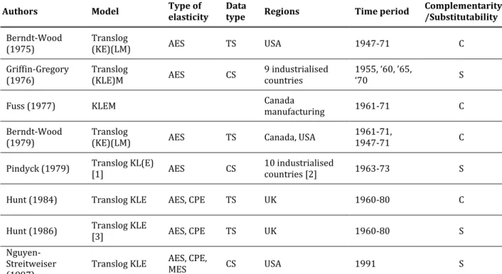
Table 1 - Early empirical studies on capital-energy substitution and complementarity
Authors Model Type of elasticity Data type Regions Time period Complementarity /Substitutability
Berndt-Wood
(1975) Translog (KE)(LM) AES TS USA 1947-71 C
Griffin-Gregory
(1976) Translog (KLE)M AES CS 9 industrialised countries 1955, ‘60, ’65, ‘70 S
Fuss (1977) KLEM Canada manufacturing 1961-71 C
Berndt-Wood
(1979) Translog (KE)(LM) AES TS Canada, USA 1961-71, 1947-71 C Pindyck (1979) Translog KL(E) [1] AES CS 10 industrialised countries [2] 1963-73 S
Hunt (1984) Translog KLE AES, CPE TS UK 1960-80 C
Hunt (1986) Translog KLE [3] AES, CPE TS UK 1960-80 S
Nguyen-Streitweiser
(1997) Translog KLE
AES, CPE,
MES CS USA 1991 S
Notes: AES: Allen Elasticity of Substitution. CPE: Cross Price Elasticity. MES: Morishima Elasticity of Substitution. TS: Time Series. CS: Cross Section. [1] The nest E includes 4 types of fuels: solid fuel, liquid fuel, gas, electricity. [2] Canada, France, West Germany, Italy, Japan, Netherlands, Norway, Sweden, UK, USA. [3] Non-neutral technical change
Considering models with three or four inputs (KLE or KLEM, respectively), the choice of including or excluding material inputs (M) implies different assumptions about the separability of the factors within production processes and, therefore, generates differences in cost shares. Indeed, as pointed out by Frondel and Schmidt (2002), the magnitude of cost shares is crucial in determining the sign for the energy price elasticity (especially in Translog estimations): higher cost shares would be more likely to determine substitutability; whereas for small cost shares it is easier to have smaller or negative elasticities (factors may be complements). As far as the
aggregation level is concerned, most of the studies have focused on the aggregate (whole
economy) level or on the industrial sector. In this regard, it should be stressed that the higher the level of aggregation and the more severe the argument will be according to which elasticity will not distinguish the pure substitution effect among factors from change in the sectoral composition of output and a shift in input demand. In fact, the measurement of elasticity of substitution assumes that there is a change in input mix keeping the level of output, which is however a homogeneous and constant product.
3.2. Energy and economic output: from Granger causality to Fully Modified OLS
Together with an analysis of short run capital-energy substitution elasticity at the aggregate level, a large strand of literature has also tried to assess the nature of the relationship between energy consumption and economic performance in the long run. Starting from Kraft and Kraft (1978), at first the goal of this line of research was to establish the direction of the causal relationship between energy consumption and output, usually measured by Gross Domestic Product (GDP), at the national level in a bivariate framework. Further econometric developments also allowed testing for non-stationarity of time series, cointegration in a multivariate setting and better controlling for omitted variables bias. Moreover, the application of panel cointegration techniques and Vector Error Correction Models (VECM) allows controlling for countries' heterogeneity and cross-sectional interdependency. Although the improvements in empirical analysis, results are still mixed and unambiguous conclusions about the direction of the causality have not yet been reached (see Ozturk, 2010 and Payne, 2010a for a review).
Investigating the role of energy in economic system in terms of direction of the causal relationship has relevant policy implications, especially considering the debate on the potential negative impact of energy and climate regulations on economic performance. The different possibilities are usually expressed in terms of four hypotheses. The neutrality hypothesis holds if no causal relationship is found between energy and economic output and suggests that energy policies have no significant impact on economic growth. On the other hand, for bi-directional causality (feedback hypothesis) energy and economic output need to be considered as interdependent because they affect each other. Considering uni-directional causality, the
conservation hypothesis is verified when the level of economic activity Granger-causes energy
consumption and, in this case, energy policies setting constraints on energy supply are considered not too harmful since the demand for energy may be mainly driven by the level of production processes or income, thus market-based measures and regulatory instruments could be used to reduce energy demand (Coers and Sanders, 2013). Finally, the growth
hypothesis is verified if causality is running from energy consumption to economic output and,
in this case, energy (together with other inputs) can be seen as a limiting factor in production processes.
If the growth hypothesis is verified, measures of intervention aimed at reducing energy consumption could negatively affect economic output while policies fostering the adoption of low carbon technologies and easier access to sustainable and clean energy supply should be preferred (Coers and Sanders, 2013). In this latter case, in particular, understanding the sign and the magnitude of the impact that energy has on the economic performances is of particular
interest (Apergis, 2013). Considering, in fact, that energy conservation policies are growing both in scope and relevance, it is crucial to determine the role that energy plays in the economic system in order to understand the potential impact of energy in different economic activities and whether energy policies can provide a positive impulse to the economic system or if they are harmful.
These studies not only apply different econometric techniques, but also cover different time periods and account for different countries, which are some of the reasons behind the diverging results. Differences in the results may also arise because countries are heterogeneous in terms of structural and development characteristics and because of the different level of aggregation analysed. In addition, there is a wide range of variables on which the analyses are performed, especially in multivariate models, and this aspect also partly justifies the diverging conclusions (Gross, 2012).
The economic variable is usually represented by GDP (in absolute value or in per capita terms) but in some cases a production index is used as an economic growth variable (Ewing et
al., 2008). On the other hand, energy is usually accounted for in terms of total final energy
consumption. In some cases primary energy consumption is used (as in Bowden and Payne, 2009), but several works also deal with particular energy resources, especially electricity (see Payne, 2010b for a review) but also coal, natural gas and fossil fuel (Ewing et al. 2009), or distinguish between renewable and non-renewable energy sources (Tugcu et al., 2012). Finally, some authors (Oh and Lee, 2004; Stern, 2000; Warr and Ayres, 2010) highlight the relevance of the composition of the energy input mix.
The level of aggregation can be seen as a further source of mixed results and contrasting outcomes may hold between the national and sectoral level analysis (Gross, 2012). In the energy-GDP cointegration analysis literature, attention has been mainly focused at the national level and only a few works investigate the relationships considering a more detailed sectoral disaggregation. Examples of country-specific studies exploring the energy-growth link at a lower aggregation level are: Bowden and Payne (2009), Ewing et al. (2009), Gross (2012), Soytas and Sari (2007), Tsani (2010), Zhang and Xu (2013), and Ziramba (2009). On the other hand, examples of multi-countries sectoral investigations are Costantini and Martini (2010), Liddle (2012), and Zachariadis (2007). However, these works usually only distinguish between residential, industry, services and transport sectors (see Table 2), and only Liddle (2012) conducts the analysis at a more disaggregated level, considering five energy intensive sub-sectors of the manufacturing industry.
Table 2 - Summary of literature review on disaggregated sectors
Study Methodology Period Country Sectors Industrial sector results
Zachariadis
(2007) VECM, ARDL, TY [bivariate]
1960-2004 G7 Total, residential, industry, services, transport different for country [1] Soytas -Sari
(2007) VECM [multivariate] 1968-2002 Turkey Manufacturing EY [2] Ewing et al.
(2008) VDC [multivariate] 2001-2006 US Industry different for energy sources Bowden-Payne
(2009) TY [multivariate] 1949-2006 US
Total, residential,
commercial, EY [3]
industrial, transport
Ziramba (2009) TY [multivariate] 1980-2005 South Africa Manufacturing different for energy sources
Costantini-Martini (2010) VECM [bivariate and multivariate] 1970-2005
71 countries Total, residential, industry, services,
transport different [4] (26 OECD and
45 non-OECD)
Tsani (2010) TY [multivariate] 1960-2006 Greece Total, industrial, residential, transport bi-directional Gross (2012) ARDL [multivariate] 1970-2007 US Total, industry, commercial, transport EY short run Liddle (2012)
[5] FMOLS 1978-2007 OECD countries 5 manufacturing sectors Zhang-Xu
(2013) VECM [multivariate] 1995-2008 China Total, industry, service, transport, residential different [6] Notes: Methodology: VECM Vector Error Correction Model, ARDL Autoregressive Distributed Lag, TY Toda-Yamamoto, VDC Variance Decomposition; G7 countries: Canada, France, Germany, Italy, Japan, UK, US; [1] more YE than EY; [2] ElectricityValue Added; [3] negative sign; [4] Bivariate model: YE in the short run, EY in the long run only for OECD sample; Multivariate model: YE; [5] Liddle (2012) has estimated the long-run elasticities for five manufacturing sectors and for the whole panel, using a panel FMOLS to estimate the parameters from a production function model; [6] YE in the short term while a bi-directional relationship is found in the long term.
In this case, determining not only the direction of the causal relationships but also the sign and magnitude of the effects that each variable has on the others is of particular importance. In fact, results can also been used to derive technological parameters to be used in empirical models (as highlighted in previous sections). The contribution by Liddle (2012) adopts the long-run relationship estimation using the Fully Modified OLS (FMOLS) estimator developed by Pedroni (2000) for heterogeneous cointegrated panel data. If the panel series are non-stationary and cointegrated, the FMOLS estimator generates asymptotically unbiased estimates of the long-run coefficients in a relatively small sample. In this case, the direction of the relationship between energy and output is assumed to be that of a production function (EY), thus generating results that can be directly interpreted in elasticity terms. More importantly, these elasticities represent a first assessment of the potential negative impact on economic output due to energy conservation policies in the growth hypothesis, providing country and sector specific assessment of the required complementary actions to be implemented to ensure energy availability (such as the adoption of low carbon technologies and easier access to sustainable and clean energy supply).
3.3. Measuring the elasticity of substitution between energy and capital at sector level
With the increasing attention that energy modelling has gained in an analysis of climate change policies, the focus of the estimations of the elasticity of substitution have moved from the complementarity or substitutability debate to econometric estimations to be implemented in applied models, so that the economy-wide structural adjustments following a change in energy price can be assessed. Although there is a long line of research in this respect, there is still no consensus on the positive or negative sign of the elasticity between energy and capital or on its magnitude. In fact, besides the theoretical assumptions exposed in the previous section, elasticity remains a relative concept (Tovar and Iglesias, 2013) and differences in the estimations are also due to different formulation models, data characteristics and estimation methods (Table 3).
Firstly, considering differences in the model formulation, there are four aspects to take into account: the number of production factors, the functional form, the formulation of the elasticity of substitution and the treatment of technological change. In relation to the former issue, and following the discussion between early works of Bernd and Wood (1975) and Griffin and Gregory (1976), empirical studies analysing substitution possibilities between energy and capital, generally take into account three or four inputs, thus distinguishing KLE and KLEM models.
Considering then the choice between different functional forms, three functions have been extensively employed in empirical analysis on capital-energy substitution: the Cobb-Douglas, the Constant Elasticity of Substitution (CES) and the Translog formulations.2 Translog production (or cost) functions, in particular, have been considered in the majority of econometric works because they have the advantage of being more flexible and, without imposing restrictions on substitutability, are more suitable when the number of inputs is greater than two. In other cases, authors have analysed CES production functions, which are a generalisation of a Cobb-Douglas form, where the elasticity of substitution is constant and not necessary equal to one but can vary between 0 and infinity. A further aspect to consider in CES functions is related to the separability assumptions, which imply different nesting structures. Differences in the aggregation of inputs can have relevant on the magnitude of substitution elasticities and, in some cases, the aim of the analysis has been an investigation into which nesting structure would best fit the data and consequently, the most appropriate elasticities estimations were selected (Kemfert, 1997).
Moreover, there are several formulations of the elasticity of substitution and, starting from
2 Further studies attempt to verify the possibility of zero substitution among inputs, according to the Leontief
function (which assumes that the elasticity of substitution is close to zero and implies that production factors need to be used in fixed proportions) or take into account Generalized Leontief functions (see Tovar and Iglesias, 2013).
the original two Hicks-type elasticity of input substitution, three main generalisations have been developed for cases with three or more factors. The Cross Price Elasticity (CPE) is at the basis of the distinction between gross and net substitution introduced by Berndt and Wood (1979) and is strictly linked with the separability conditions assumed in the model. In particular, in KLEM models, taking E and K as separable from L and M, the CPE is an asymmetric
one-factor-one-price elasticity that represents the net substitution between E and K and measures the relative
change in use of one factor (K) given a change in the other factor’s price (E), keeping output and other input prices fixed. It is the sum of the positive gross price elasticity (which measures the change in E and K demand, holding EK composite input fixed) with the negative expansion elasticity, whose magnitude depends on the cost share of K (in this case output is fixed but the demand for the composite input EK can vary in response to changes in relative prices). Complementarity or substitutability depends on which of the two effects is larger, and the cost share of the two factors have a crucial role, thus changes in energy or capital prices will have different consequences also due to the fact that the capital cost share is usually higher than the energy one.
The Allen Elasticity of Substitution (AES) has been widely used in empirical studies and, as for the CPE, a positive value implies an increase in the use of one factor as a consequence of the increase in the price of another factor, and corresponds to the substitutability case among inputs. Contrary to CPE, it is a symmetric one-factor-one-price formulation that measures the effect of changes in price i on the demand for input j, taking into account the share of input j in output value. Indeed, it can also be derived by dividing the CPEij by the cost share j (Broadstock
et al., 2007).
The Morishima Elasticity of Substitution (MES) is an asymmetric measure of substitution between production factors and, in contrast to AES and CPE, is a two-factor-one-price elasticity that represents the change in the ratio of factor quantities given a change in one factor prices. It is positive in almost all cases and the sign is therefore not very useful for distinguishing substitution from complementarity. Moreover the cost share i will decrease relatively to j (following a rise in pj) only when MES>1. Blackorby and Russel (1989) show that the MESij can be calculated as the difference between the CPEij and the own price elasticity for input j (CPEjj). As far as AES is concerned, if two inputs are Allen substitutes they will also be MES substitutes, but when AES is negative it is still likely to have positive MES.
A further aspect to take into account, which has already emerged in the early debate, is the way technological change is treated. Generally represented in the Hicks-neutral form, technical change can also be represented as non-neutral or factor saving, as in Hunt (1986), Kemfert (1997), Morana (1998), Su et al. (2012), and van der Werf (2008). Moreover, in some cases, non-constant returns to scale are implemented, and Koetse et al. (2008) show that including
returns to scale parameters has a positive and significant impact on MES and CPE. In other studies, as in Popp (1997), a time trend is used to approximate the effect of a general technological change, but it cannot be specifically related to innovations fostering specific forms of energy efficiency. It is also worth noting that non-exogenous technical change can be derived from both factor substitution, as a response to changes in price or income, and capital accumulation, representing innovation embedded in new production machines. Moreover, factor substitution at the aggregate level can be seen as a change within the same technology but, at the process-engineering lower level, it still implies a shift in technologies (Jacoby et al., 2004).
Estimates also vary according to the data characteristics, in term of regions, sectors and time periods selected. In some cases, analysis is focused on a single country, US and UK above all (Broadstock et al., 2007), while in others a sample of countries is analysed, in a cross-section or panel framework. Different results can also arise from different time horizons considered, especially when the time period is quite long and includes some structural breaks that could have modified economic behaviour with regard to energy demand and consumption. Examples of this are oil shocks from the '70s or the introduction of policies able to substantially affect economic activities as far as capital-energy substitution is concerned.
A further source of variation can also be ascribed to the way production factors are measured. In particular, most works consider aggregate energy consumption whereas in other cases specific energy fuels or electricity are distinguished. Moreover, a consequent and relevant argument in the elasticity debate concerns the substitution possibilities at a lower level than the capital-energy nest, or rather between different types of energy inputs, such as electricity, fossil fuels or renewable energy, as in Halvorsen (1977) and Morana (1998). In this regard, Bacon (1992) and Stern (2012) proposed, respectively, a review and a meta-analysis on inter-fuel substitution. As far as capital input is concerned, different types of measure can be accounted for. Tavor and Iglesias (2013), for example, distinguish capital input in buildings from machinery and equipment, whereas Kim and Heo (2013) account for two forms of capital, the first increases the electricity demand while the second does not, while energy is divided into electricity and fuels (they calculate specific capital-fuel elasticity and find evidence of asymmetric substitution).3
3 Energy substitution for capital is greater than the inverse case, i.e. capital do not substitute for energy in the
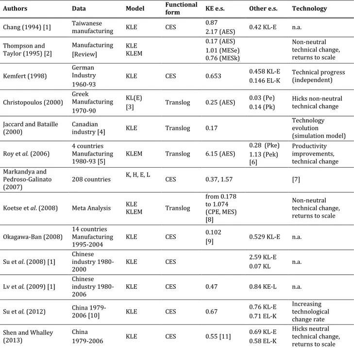
Table 3 - Review of aggregate capital-energy elasticity of substitution estimates
Authors Data Model Functional form KE e.s. Other e.s. Technology
Chang (1994) [1] Taiwanese manufacturing KLE CES 0.87
2.17 (AES) 0.42 KL-E n.a. Thompson and Taylor (1995) [2] Manufacturing [Review] KLE KLEM 0.17 (AES) 1.01 (MESe) 0.76 (MESk) Non-neutral technical change, returns to scale Kemfert (1998) German Industry 1960-93
KLE CES 0.653 0.458 KL-E
0.146 EL-K Technical progress (independent) Christopoulos (2000) Greek Manufacturing 1970-90 KL(E) [3] Translog 0.25 (AES) 0.03 (Pe) 0.14 (Pk) Hicks non-neutral technical change Jaccard and Bataille
(2000) Canadian industry [4] KLE Translog 0.17
Technology evolution
(simulation model) Roy et al. (2006) 4 countries Manufacturing
1980-93 [5] KLEM Translog 6.15 (AES)
0.28 (Pke) 1.13 (Pek) [6] Productivity improvements, technical change Markandya and Pedroso-Galinato (2007) 208 countries K, H, E, L CES 0.37, 1.57 [7]
Koetse et al. (2008) Meta Analysis KLE KLEM Translog
from 0.178 to 1.074 (CPE, MES) [8] Non-neutral technical change, returns to scale Okagawa-Ban (2008) 14 countries Manufacturing
1995-2004 KLE CES
0.102
[9] 0.529 KL-E n.a. Su et al. (2008) [1] Chinese industry
1980-2000 KLE CES
2.59 KL-E 0.07 KL n.a. Lv et al. (2009) [1] Chinese industry
1980-2006 KLE CES 0.47 0.84 KE-L n.a.
Su et al. (2012) China 1979-2006 [10] KLE CES 0.67 0.76 KL-E 0.71 EL-K
Increasing technological change rate Shen and Whalley
(2013) China 1979-2006 KLE CES 0.55 [11] 0.69 KL-E 0.58 EL-K Hicks neutral technical change, returns to scale Notes. [1] Estimations from Su et al. (2012); distinctions between E.S formulations not available. AES values are derived from Markandya-Pedroso Galinato (2007). [2] The review analyses several studies different for KLE or KLEM model, functional forms. MESi represents the Morishima E.S. when the price of input i alters. [3] Price index of energy (E) is constructed aggregating Electricity (EL), Diesel (D), Crude oil (M). Results in table are, Allen E.S. and Price elasticity corresponding to a change in price of factor i (Pi). [4] Pseudo data. They also estimate aggregate EK elasticities for commercial 0.34, residential 0.21, Canada total 0.24. [5] The study includes 3 developing countries (South Korea, Brazil, India) and USA. [6] Results in table are, Allen E.S. and Price elasticity, relative to country pooled estimates. AES excluding Brazil is 4.72. [7] Produced capital (K), Human capital (H) measured as Intangible capital residual (HR) or human capital related to schooling (HE), Energy (E) including oil, natural gas, hard coal and lignite, Land resources (L). Results in table are from the four-factors (KEH)L model using HR and HE. Estimate for the two-factors model with capital and energy using HR is -0.48 but not significant. Estimates using HR (HE) in the three-factors (KE)L model is 0.65 (0.17). The authors did not consider technology, but they include indicators for institutional development and efficiency of economic organization and use non-linear estimation method to estimate the CES function. [8] Different for: Long and short run, Europe and North America, pre-1973, post-1973 and post-1979, MES or CPE. The range reported in Table 3 includes only significant estimates. [9] Result in table is for manufacturing industry, for sector specific elasticities see Table 4. [10] Elasticities for different time periods are, respectively, for 1953-1978 period and 1953-2006: KE 0.2152 and 0.2826; KL-E 0.2553 and 0.2599; EL-K 0.3177 and 0.3329. The authors use nonlinear regression carried on different optimization methods. [11] Results in table are the average elasticities calculated from estimations with constant and non-constant returns to scale for both (K, HL, E) and (K, L, E) models. The authors use grid search based non-linear estimation procedures.
Finally, different data characteristics require different (econometric) estimation methods, especially considering the increasing number of panel data studies. Differences in results can also be due to: linear or non-linear methods, static or dynamic models, non-stationarity and cointegration in time series, correlation between regressors and error components, endogeneity, omitted variable bias4 or the choice of panel estimators (pooled OLS, Fixed or Random Effects, Between estimators).
Koetse et al. (2008) present a meta-analysis on capital-energy substitution elasticity (focusing on CPE and MES) to explain the heterogeneity between different studies and also calculate short and long run elasticities for different regions and time periods. If the exclusion of materials5 (KLE function) and the inclusion of non-neutral technical change do not seem to significantly affect estimation results, the assumption of non-constant returns to scale has a significant and positive effect. Moreover, cross section data (long-run elasticity) and, for CPE, also aggregate data (in contrast with 2- or 4- digit manufacturing data) produce higher elasticities6. With respect to regions and time period, estimations for Europe tend to be lower than the US and systematic differences seem to arise from data before or after the two oil crises (1973, 1979). Aggregate measures of inputs (with respect to CPE) can also lead to underestimating the substitution possibilities since both coefficients for energy fuels and machinery (instead of aggregate E and K) are significant and positive whereas electric energy has a negative coefficient. Given all these possible sources of differences, in order to define a reference range of variation for the capital-energy elasticity of substitution, studies with similar characteristics of interest have to be picked. Here, the research focus is on the level of disaggregated sectors in manufacturing industry and previous attempts studying the substitution elasticity between E and K in this respect are presented in Table 4.
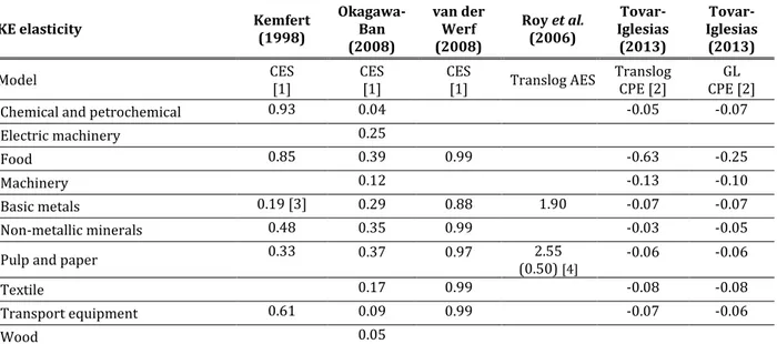
Kemfert (1998) analyses data for industry in West Germany from 1960 to 1993, also accounting for 7 sectors in manufacturing industry (1970-1988)7, and tests which nesting structure of a CES function with three inputs would best fit the data (using non-linear estimation methods). For the aggregate industry the (KE)L nesting form gives the highest R-sq whereas for all industrial sectors (except for food), the (KL)E structure seems more appropriate. Considering both capital-energy elasticity from the first nesting structure and (KL)E elasticity from the second, energy and capital are substitutes for all sectors with ranges of variation going, respectively, from 0.04 to 0.93 and from 0.35 to 0.97.
4 Most relevant omission bias can be ascribed to a lack of information on the technology status and even the inclusion
of a (deterministic) time trend is just an approximation.
5 Also Roy et al. (2006), studying a KLEM Translog function without imposing any separability assumptions and then
testing different restrictions, find weak evidence in this respect.
6 Higher elasticity values from cross section data, and lower ones for time series cases, was the argument proposed
by Griffin and Gregory (1976) and also adopted by Koetse et al. 2008 to calculate (cross section) long-run and (time series) short-run elasticities.
Okagawa and Ban (2008) estimate substitution elasticities to be implemented in a CGE model considering a three level nested CES function (KLEM). They focus their attention on two main structures, the KE-L and KL-E forms, using data from 14 countries8 and 19 industries (within which there are 10 manufacturing sectors)9, from 1990 to 2004. From the former model they obtain EK elasticities ranging from 0.04 to 0.45 (where the assumed pre-existing parameters were 0.10 or 0.20), while in the latter, the (KL)E elasticities go from 010 to 0.64 (while the pre-existing parameters were equal to 0.4 for all sectors)11; they also find higher KE elasticities for energy-intensive industries. The comparison of results from a GAMS/MPSGE static CGE simulation with the estimated parameters shows that, in order to cut CO2 emissions by 13% in Japan, in the (KE)L form the carbon tax required is 44% lower than with the original parameters.
Van der Werf (2008) conducts an empirical analysis on 12 OECD countries (1978-1996) accounting for the manufacturing industry and 6 sub-sectors12, along with the construction industry, and estimates (sector and country specific) substitution elasticities to be implemented in dynamic climate change models. Considering industry specific results, in the (KL)E structure the elasticity between energy and aggregate input (in this case KL) varies between 0.17 and 0.64, in the (LE)K case from 0.18 and 0.50 whereas in the (KE)L form, values for capital-energy elasticity of substitution are significantly higher and around unity (from 0.96 to 1.00).
Tovar and Iglesias (2013), using data from 8 UK manufacturing industries13 from 1970 to 2006, estimate capital-energy cross price elasticities (CPE) from two flexible forms, i.e. Translog and Generalized Leontief functions, and account for technological change by introducing a time trend. They account for 5 production factors: labour, energy, materials and two types of capital input, buildings and machinery and equipment. In the Translog KLEM model, energy and capital are complements in each sector (elasticities for buildings are higher in absolute value), but when materials are dropped (KLE model) estimates are only significant and negative for machinery. When using the GL function (however, in the Translog model, the goodness of fit is higher), capital-energy elasticities in the long-run are all negative and, in particular, chemical, machinery, textile and food sectors show higher absolute values while short-run values are
8 Austria, Belgium, Denmark, Finland, France, Germany, Japan, Italy, Luxembourg, Netherlands, Spain, Sweden, UK
and US.
9 Manufacturing sectors considered in the analysis by Okagawa and Ban (2008) are: Food, Textile, Wood, Pulp and
paper, Chemical, Other non-metallic mineral, Basic metals, Machinery, Electrical equipment and Transport equipment.
10 For Chemical sector the (KL)E substitution elasticity reported in the Appendix is negative (-0.065) but in the result
section is reported as 0.
11 To resume, previously assumed elasticities were: for KE-L model 0.80 (KL-E) and 0.10 or 0.20 (KE); for KL-E model
0.40 (KL-E) and 1.00 (KL).
12 Basic metal products, construction, food and tobacco, textiles and leather, non-metallic minerals, transportation
equipment, and the paper, pulp and printing industry
13 Basic metals, chemical and petrochemical, non-metallic minerals, transport equipment, machinery, textiles, food