DOTTORATO DI RICERCA IN INFORMATICA
Ciclo: XXVI
Settore Concorsuale di afferenza: 01/B1
Settore Scientifico disciplinare: INF01
Automatic Deployment of
Applications in the Cloud
Presentata da: Tudor A. Lascu
Coordinatore Dottorato:
Relatore:
Maurizio Gabbrielli
Gianluigi Zavattaro
Abstract
In distributed systems like clouds or service oriented frameworks, applications are typically assembled by deploying and connecting a large number of heterogeneous software components, spanning from fine-grained packages to coarse-grained com-plex services. The comcom-plexity of such systems requires a rich set of techniques and tools to support the automation of their deployment process. By relying on a formal model of components, a technique is devised for computing the sequence of actions allowing the deployment of a desired configuration. An efficient algorithm, working in polynomial time, is described and proven to be sound and complete. Finally, a prototype tool implementing the proposed algorithm has been developed. Experi-mental results support the adoption of this novel approach in real life scenarios.
A Paola, la mia compagna di vita, va il primo e pi`u grande grazie. L’appoggio che mi ha dato in questi anni `e stato essenziale. `E stata la prima persona a farmi capire che la cosa pi`u importante `e stare bene con se stessi. La vita con te e Federico `e piena di gioia.
Per quanto riguarda l’ambiente universitario, sono tante le persone cui devo molto. Prima di tutto, il Professor Cosimo Laneve per aver creduto in me ed avermi convinto che ero in grado di intraprendere il percorso di dottorato. Senza di lui non l’avrei fatto e gliene sono riconoscente.
Ringrazio i Professori Gabbrielli, Martini e Sangiorgi che, abbinando un grande valore umano ad un grande valore professionale, mi hanno aiutato a superare i momenti di difficolt`a del mio percorso.
Ringrazio il Professor Gianluigi Zavattaro che ha accettato di “adottarmi scien-tificamente” e che mi ha sempre accolto con un sorriso.
Ringrazio la Professoressa Vania Sordoni che `e sempre stata una figura amica, a partire dalla stesura della tesi di laurea in poi. `E bello passare qualche volta a fare quattro chiacchere in simpatia.
Ringrazio i miei compagni di sventura Ornela, Andrea, Giulio, Andrea B., Armir e Nicol`o che nel corso delle scuole estive e dei corsi di dottorato sono stati un gruppo simpatico ed affiatato. In particolare, un grosso grazie a Giulio per la compagnia e le innumerevoli chiaccherate alla macchina del caff`e.
Ad Elena devo di avermi mostrato che si pu`o fare ricerca con passione ed avere una famiglia, allo stesso tempo.
A Jacopo devo di avermi mostrato cosa vuol dire determinazione e continuit`a (e puntualit`a). Grazie anche per avermi s{u,o}pportato come collega di lavoro gomito a gomito.
A Sara devo di tener presente sempre e comunque che siamo prima di tutto esseri umani.
Grazie a tutti i ragazzi dell’underground, vecchie e nuove leve, per la simpatia che mi hanno sempre mostrato: Ivan, Marco, Luca, Saverio, Valeria, Silvio, Roberto, Francesco.
Grazie a Miriam, Daniela, Paolo, Lucia e Vito per aver contribuito a dare una certa atmosfera che mi mancher`a.
Grazie ad alcuni ex compagni di studio, Andrea Bagnacani, Matteo Acerbi e Michele Alberti, che hanno ancora voglia di passare a trovarmi.
Ringrazio i membri del progetto Aeolus, in particolare il gruppo di Parigi che mi ha ospitato per il periodo all’estero: Roberto Di Cosmo, Stefano Zacchiroli, Michael Lienhardt, Jakub Zwolakowski, Pietro Abate e Ralf Treinen. Il Professor Roberto Di Cosmo mi ha mostrato che si pu`o essere brillanti con semplicit`a e umilt`a. Grazie a Zack per la disponibilit`a e per avermi aiutato a cavarmela nella vita di tutti giorni a Parigi. Grazie a Pietro per la pazienza e per avermi svelato l’esistenza di ocamlbuild. Grazie a Michael per le chiaccherate durante le pause e per aver sempre cercato di stimolarmi a lavorare, anche quando non ne avevo voglia.
Grazie, infine, ai Professori Jean-Bernard Stefani e Di Cosmo per aver letto con attenzione la tesi ed avermi inviato dei commenti utili.
Per quanto riguarda il mondo “fuori” da quello accademico, ringrazio: Alina, Andrei e Marco; gli amici “da sempre” Paolo, Michele, Giacomo e Stefano; Cristiana e Gabriel; Steve e Beverly; Alessandro; Matteo; Giuliano; Fra e Mari; Camillo; Cecilia. Persone care che ci sono sempre e sempre ci saranno.
Un ultimo caloroso pensiero va ad alcune persone che significano tanto per me e che sono venute a mancare, ma non per questo meno presenti: Mariolina, Pierre e mio pap`a, colonna portante della mia vita.
Contents
I
Preface
1
1 Introduction 3
II
Background
6
2 Scenario 7
3 State of the art 9
3.1 Academia . . . 11
3.2 Industry . . . 19
4 Elements of planning theory 27
III
Model
33
5 The original Aeolus model 35
5.1 Decidability and complexity . . . 43
5.2 Other component models . . . 45
6 Theory 51
6.1 Aeolus− model & problem statement . . . 51
6.2 Technique . . . 56 6.2.1 Reachability analysis . . . 61 6.2.2 Abstract planning . . . 65 6.2.3 Plan synthesis . . . 72 6.2.4 Heuristics . . . 80 6.3 Formal analysis . . . 82
6.3.1 Soundness & completeness . . . 82
6.3.2 Computational complexity . . . 88
7 Practice 93 7.1 METIS: a deployment planner . . . 93
7.2 Validation . . . 95
V
Conclusion
113
8 Future directions 115 8.1 Integration in the Aeolus toolchain . . . 1158.2 Conflicts . . . 117 8.3 Capacity constraints . . . 120 8.4 Heuristics . . . 121 8.5 Reconfigurations . . . 121 8.6 Restrictions . . . 122 9 Concluding remarks 123 References 131 vi
Part I
Preface
Chapter 1
Introduction
Deploying software component systems is becoming a critical challenge, especially due to the advent of cloud computing technologies that make it possible to quickly run complex distributed software systems on-demand on a virtualized infrastructure, at a fraction of the cost which was necessary just a few years ago. When the number of software components, needed to run an application, grows and their interdepen-dencies become too complex to be manually managed, it is necessary for the system administrator to use high-level languages for specifying the system’s requirements, and then rely on tools that automatically synthesize the low-level deployment ac-tions necessary to actually realize a correct and complete system configuration that satisfies such requests.
Automation is thus a key ingredient for a wide adoption of cloud facilities. It appears at multiple levels ranging from the installation of packages to scaling com-puting power (like increasing the number of virtual machines).
In order to deploy an application one needs to specify a sequence of actions like creation/deletion of components, wiring of components (component functionalities), and internal steps to be carried out by each component employed. Moreover, the order in which these actions are to be performed is crucial as it ensures the correct-ness of all intermediate configurations that the system undergoes. Such a sequence of actions is called a deployment plan.
complex systems, assembled from a large number of interconnected components, is a serious challenge. This is the goal of the thesis and constitutes the main contribution of this dissertation. The work has been developed as part of the Aeolus research project [1] 1. The problem is cast in the Aeolus component model [30], specifically tailored to describe uniformly both fine grained software entities, like packages in a Linux distribution, and coarse grained ones, like services, obtained as composition of distributed and properly connected sub-services.
A novel approach for the automatic synthesis of deployment plans has been developed. The technique is shown to be correct, by proving its soundness and completeness, and efficient (of polynomial computational complexity). Moreover, viability in practice of the proposed technique is assessed by means of a proof of concept implementation, validated against standard planning techniques.
Thesis structure. Part II gives an overview of the context for this work. Chap-ter 2describes the typical usage scenario, Chapter3summarizes the state of the art solutions from both academia and industry, Chapter 4provides some basic elements of planning theory (that will be of use in the validation part).
PartIIIdescribes the original Aeolus component model and reports formal results proving the impossibility to find efficient solutions to the problem of interest, in the general case. In the end, some related component models are recalled.
PartIV is the key part, dedicated to the main contribution of this dissertation, first focusing on the theoretical aspects (Chapter6) and then on the practical issues (Chapter 7). Chapter 6 starts by presenting Aeolus−, a meaningful restriction of the original model, that allows us to devise an efficient algorithm to deal with the problem of interest. The formal statement of the deployment problem, the one we aim to solve, is given. It then continues with the description of the technique developed to tackle the deployment problem together with formal results for its soundness, completeness and efficiency. Chapter 7 deals with the presentation of METIS, a prototype tool, implementing the devised technique, and its validation.
Chapter 1. Introduction 5
Part V closes the dissertation by outlining future directions of development for the presented approach (Chapter8) and by drawing some concluding remarks (Chap-ter 9).
Background
Chapter 2
Scenario
In the cloud era, deploying a complex application on commodity (physical or virtual) machines is becoming more and more a common task. This is due to many different reasons such as cost-effectiveness, scalability, etc. . . The elastic computing paradigm enables rapidly adapting an applications’ needs to the real usage. It might be cheaper to rely on commodity hardware instead of buying and maintaining it in-house.
In the current setting every organization that needs to perform often this task, typically has a team of experts that establishes how the different components are to be installed and connected together. That is, they find a sequence of actions, a deployment plan, that when performed, permits to achieve the desired system. This part of the work is usually performed by hands with “paper and pencil”. The deployment process is then automated by coding it in custom scripts. This approach, however, is effective only if the architecture of the system is decided once and for all. Todays’ applications, however, are expected to change at a very high pace as it is common practice to switch to a different service delivering the same required functionality. In fact, for the same functionality different competitors show up on the market everyday and can quickly become appealing. If the system is subject to change the “by-hands approach” does not scale, resulting in a lot of time spent patching the custom scripts to adapt the deployment plan to the new component. This is rather unsatisfactory as a business process and it is natural to ask for a better solution.
The Aeolus project aims to develop techniques and tools, ground on solid scien-tific bases, to enable simplifying the management of systems/applications to be put in production in the cloud. One of the key ingredients to reach this ambitious goal is a suitable technique to automate the deployment process.
As an example of a possible scenario, one can consider the deployment of Word-Press, a popular blog platform. First, an installed Apache web server is needed to be able to install WordPress. In order to activate the latter one must first ensure that all services required are up and running and that they are all properly connected. Bringing it in production requires also to activate the associated service. WordPress, for instance, must connect to an active MySQL node. In fact, WordPress cannot be started before MySQL is running. This is precisely the kind of temporal dependen-cies taken into account by a deployment plan. Such a plan for this basic example would specify the following steps: first, install and activate an Apache server; install WordPress; install and activate a MySQL instance; finally, connect Wordpress to to the MySQL node and activate WordPress.
Chapter 3
State of the art
Deployment automation is among the key ingredients of the “cloud promise”. In fact, the last years have witnessed a constant rise in the interest towards automation of the process for managing a system in the cloud, both in industry and academia. This is testified by many efforts from both worlds to bridge the gap from the tradi-tional/custom way of dealing with the problem to a rich set of techniques and tools enabling a higher level of automation. Managing the installation of an application in the cloud is a process crossing many related areas such as system’s deployment, configuration and management.
Currently, developing an application for the cloud is accomplished by relying on either of the following service models: Infrastructure as a Service (IaaS) or Platform as a Service (PaaS). The aim of the former is to provide a set of low-level resources forming a “bare” computing environment like CPUs, memory, network, etc . . . The latter, instead, is meant to provide a full development environment where some mid-dleware services are already accessible (operating system, development kit, runtime libraries, etc . . . ).
For IaaS, at the beginning the intended usage scenario was the following: the de-veloper would pack the whole software stack into a virtual machine, containing the application and all its dependencies; the virtual machine would then be hosted on an virtual/physical machine on the provider’s cloud. This paradigm however is limited to cases in which the application is not subject to frequent change. In case this does
not apply, the cost of rebuilding from scratch the virtual machine with the whole software stack can become a heavy burden. Another deployment approach, based on IaaS and gaining more and more credit, is the one put forth by the DevOps [3] com-munity. Following this approach an application is developed by assembling available components that serve as the basic building blocks. This emerging approach works thus in a bottom-up direction. From individual component descriptions and recipes for installing them, an application is built as a composition of these recipes. The latter may be seen as deployment plans for individual components and the “global” deployment plan becomes thus the composition of individual ones.
In the PaaS setting, instead, applications are directly written in a programming language supported by the framework offered by the provider, and then “pushed” to the cloud. It is then up to the provider to set up the necessary run-time environment to execute the newly created application. Almost all details of the deployment are handled automatically. The PaaS approach seems promising, as it lifts the level of abstraction, but at the moment the solutions it provides are limited and thus does not represent a valid alternative for the scenario taken into account by our work. In fact, the high-level of automation comes at the (high) price of little flexibility in choosing the components that the developer may use. First of all, the choice of the programming language to employ is restricted to the ones supported by the specific PaaS provider. Moreover, the application code must conform to specific APIs. Google App Engine [4], one of the most successful products in this setting, supports only applications written in Java and Python 1 and in the Java code, threads are not allowed. Another example of the lack of flexibility in the PaaS world is given by Windows Azure [11] that works only with applications built on proprietary technologies. Moreover, the PaaS setting can be seen as a “middleware as a service” solution. Application stacks are thus limited by the middleware services supplied by the PaaS provider. This makes it unfit, at least at present time, for the high degree of customization demanded by ordinary application stacks.
A third way to deal with deploying applications in the cloud is the one employed
Chapter 3. State of the art 11
by so called holistic frameworks, such as TOSCA [64, 19, 76] and Blueprints [67]. This is a model-driven approach where an application is defined in terms of a high level description. A projection process is thus enabled where the deployment plan for the full application is generated in a top-down way. 2 From the private sector, among the others adopting this approach, we can cite IBM SmartCloud Orchestrator [48]. As we will detail in Section6.2, the approach that we propose shares some com-monalities with the above ones and it might actually be conceived as an intermediate way between the full bottom-up and top-down approaches. The description of the application is a high-level one but the deployment plan is inferred from a declarative description of individual components, forming the basic building blocks.
In the following we review state of the art solutions by discussing first works from academia and then tools made available in the industry.
3.1
Academia
Engage
Engage [34] is a deployment management system. Throughout the paper the term resource is used as a synonym of component. Every resource is represented by two parts: a declarative one, the type, and an implementation part, the driver. The former is employed to statically verify deployment properties and to generate the deployment plan, while the latter, implemented in a specific language, provides all the required low-level actions to install and manage the resource’s life cycle. A notion of hierarchy is introduced by employing three kinds of dependencies: Inside models nesting of resources (like a program running into an application server); Env models local dependencies, that is resources that the current one requires to find on the same physical or virtual machine (like a program needing a Java execution environment); Peer models dependencies to resources possibly deployed anywhere else (one has to look inside and outside the machine of the resource under consideration).
2In order to achieve this some form of recipe for the deployment of the bottom level components is obviously necessary.
Figure 3.1: Example of hypergraph generated by Engage.
The workflow of the Engage framework is the following. There is a universe of available resources populated by the community (typically the vendor of an applica-tion writes down the resource type and the driver for its product). A user writes a (partial) specification of the system he wants to deploy using the resources available in the universe. This (partial) specification is then fed to Engage that first verifies some correctness properties: it mainly amounts to verify that the union of the three dependency relations is acyclic. This is crucial as we will soon explain. The second step is the generation of a hypergraph where nodes and edges represent respec-tively resource instances and dependencies (each edge is labelled with the kind of dependency). Hyperedges are used to model disjunction of dependencies: a resource requires a functionality provided by two or more resources.
Figure 3.1 depicts an example of the generated hypergraph. In this example the Tomcat resource requires a Java environment to execute, this can be provided by a JRE or by a JDK as shown by the hyperedge, tagged with env, to these two resources.
A topological sort of the hypergraph is used to extract an installation order for the deployment plan of the resource instances in the desired system. The acyclicity of the dependency hypergraph ensures that a topological sort exists, thus guaranteeing that a suitable order can always be found. From the hypergraph a set of Boolean constraints is then generated and given as input to a SAT solver. The solution found by the solver corresponds to a 0 − 1 assignment to every resource instance, telling us if it needs to be installed or not. This information is then put together with the installation order given by the topological sort of the hypergraph to obtain a full
Chapter 3. State of the art 13
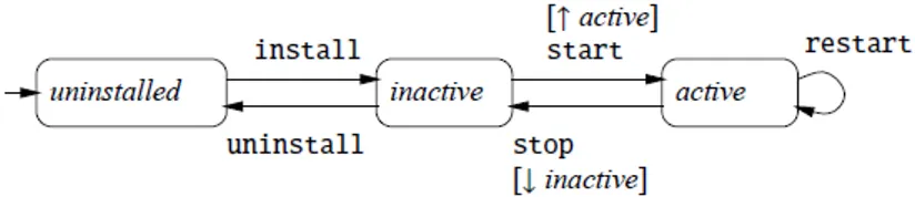
Figure 3.2: Typical state machine associated to a resource driver.
deployment plan.
In the last phase this plan is actually carried out using the driver of each resource. Each resource driver can be seen as a state machine that defines the lifecyle of a resource of that kind. Each driver is thus made of states and transitions. The set of states must contain at least the uninstalled, inactive and active states. Transitions between states take the form of guarded actions [↓ s] α or [↑ s] α, where s is a boolean condition, the ↓ and ↑ arrows define its scope and α is an action that is fired when the transition is taken. The ↑ arrow means that condition s has to be fulfilled by all the resources upon which the given resource depends on (its upstream dependencies) while the ↓ arrow means that condition s has to be fulfilled by all the resources that depend on the given one (its downstream dependencies). If and when condition s becomes true then action α is triggered and the transition is fired, otherwise it stays pending.
In Figure 3.2 a typical state machine of a resource r is depicted. Notice that the start action and the corresponding transition can be fired only when all the resources that r depends on are already active.
The Engage model introduces some important simplifications in order to reach a feasible solution. First of all, conflicts and capacity constraints are not modeled. The acyclicity constraint, crucial to the Engage approach, banishes the possibility of having resources that are mutually dependent, a common case in real-world appli-cations. Moreover, dependencies are between resources, regardless of their current state. i.e. the granularity of dependencies is coarse. The guarded actions are limited in their scope: the only two possibilities are downstream and upstream. Finally, an
Figure 3.3: ConfSolve workflow.
underlying assumption is that the state machine in a driver forms a strongly con-nected graph (as each state is required to be reachable from any other in the state machine).
Overall, Engage represents an interesting compromise between applicability and efficiency but for the deployment problem in the cloud.
ConfSolve
The aim of ConfSolve [44, 45] is to define a suitable language for the description of problems related to system’s configuration. The sought language should be de-signed to ease stating such problems, on one side, and enable their translation into constraint satisfaction problems (CSPs), on the other. This way one can rely on tech-niques from the CSP world to tackle the problems of this domain. ConfSolve consists basically into a definition of a domain specific language and translation mechanisms to a popular format for the description of CSP problems, namely MiniZinc [62]. The underlying assumption is that specific problems can be naturally modeled (and thus expressed) as constraints over valid configurations.
Figure 3.3 shows the ConfSolve workflow. First a specification is written down in the ConfSolve language. This specification defines both the model and the con-straints over it that will specify what is a “valid configuration”. The specifica-tion is translated by a compiler into the MiniZinc model. This in turn is “flat-tened”/translated into a FlatZinc model by a third-party compiler. The obtained problem is then fed to a third-party CSP solver, in this case the chosen one is Gecode [36] but this is a completely modular choice (no changes are needed as long as the solver accepts FlatZinc problem definitions). Finally the solution found by the solver is translated back into a ConfSolve instance. This represents a valid
con-Chapter 3. State of the art 15
figuration that optimizes one or more parameters chosen to define the configuration management problem of interest. As an example one can think of the problem of maximizing the number of (possibly many kinds of) virtual machines per physical one.
The aim of the ConfSolve research was defining a language that would allow to express typical configuration management problems, with direct translation mech-anisms to popular formats for stating CSP problems. The ConfSolve language is object oriented and declarative. The ConfSolve specification is a collection of class declarations, enumerations, variables and constraints where the order in which they appear does not matter. Association between objects and names is achieved through the use of reference variables. Declaration var host as ref Machine;, for instance, states that host is a reference to an object of type Machine. Each reference, left unassigned by the user, represents a decision variable, that will be instantiated by the solver according to the specified constraints. This constitutes the key idea behind ConfSolve: the system administrator is provided a specific language for defining con-figuration problems so that solutions can be represented as assignments over some decision variable(s). The language allows using quantification and summation over decision variables in constraints.
f o r a l l ws in w e b S e r v e r s w h e r e ws . h o s t != m0 {
ws . p o r t = 8 0;
}
Above code for example, may be used to require that every element in webServers, not running on host m0, has port set to 80. As for summation consider the following code: w h e r e f o r e a c h ( m in m a c h i n e s ) { sum ( r in r o l e s w h e r e r . h o s t == m ) { r . cpu } <= m . cpu }
where the above constraint is specifying that for each physical machine if we sum the CPU power of the virtual machines deployed, the total amount does not exceed the capacity bound.
Finally there is also the possibility of writing optimization constraints that instan-tiate decision variables in way to maximize (or minimize) a given expression.
The major limitation of this approach is that the ConfSolve language models faithfully the problem of optimal provisioning (of virtual machines) rather than focusing on the deployment process. For instance, it does not take into account the wiring aspect, i.e. how to bind the components in use. The steps needed to reach the final (optimal) configuration computed by the solver are also out of scope.
VAMP
VAMP (Virtual Applications Management Platform) [33, 71] is a framework that enhances automatic configuration of a distributed application in the cloud. The framework is made of the following elements: a language to describe the global structure of the application and an environment to manage the runtime deployment of components. The language extends the OVF (Open Virtualization Format) [31] language, that is a proposed standard 3 for a uniform format for applications to
be run on virtual machines. The OVF descriptor is an XML file describing the structure of the application. VAMP extends the descriptor with sections that specify the architectural view of the distributed application: interfaces, dependencies and bindings. Listing 3.1 shows a sample AppArchitectureSection section contained in the extended OVF descriptor.
The deployment process is then implemented as a decentralized protocol in a self-configuration manner. The approach is interesting but limited for our purposes as it works under the assumption that the dependency graph is acyclic. 4 Another limitation is given by the fact that the developer must specify the virtual machine
3Promoted by the Distributed Management Task Force (DMTF).
4Dependencies can be optional or mandatory (needed for component activation). It is assumed that there is no cycle among mandatory dependencies.
Chapter 3. State of the art 17
Listing 3.1: Added section to OVF descriptor
1 <! - - A p p l i c a t i v e a r c h i t e c t u r e - - > 2 < A p p A r c h i t e c t u r e S e c t i o n > 3 < d e f i n i t i o n n a m e =" T o k e n A p p " > 4 < c o m p o n e n t n a m e =" C0" > 5 < i n t e r f a c e n a m e =" c " r o l e =" c l i e n t " .../ > 6 < i n t e r f a c e n a m e =" s " r o l e =" s e r v e r " .../ > 7 ... 8 < virtual - n o d e n a m e =" VM0"/ > 9 </ c o m p o n e n t > 10 < c o m p o n e n t n a m e =" C1" > 11 ... 12 </ c o m p o n e n t > 13 < c o m p o n e n t n a m e =" C2" > 14 ... 15 </ c o m p o n e n t > 16 < b i n d i n g c l i e n t =" C0. c " s e r v e r =" C1. s " / > 17 < b i n d i n g c l i e n t =" C0. c " s e r v e r =" C2. s " / > 18 ... 19 </ d e f i n i t i o n > 20 </ A p p A r c h i t e c t u r e S e c t i o n >
in which a given component lives (see line 8 in the above code) : ideally, from our perspective, this is part of low level details that one may not care when defining an application.
A Formal Framework for Component Deployment
In [56] a framework has been developed to formally frame the problem of component deployment. The aim of the work is to model the deployment process of component systems and, based on this, to define a technology-agnostic technique to ensure some correctness properties.
To this purpose a Labeled Transition System (LTS) is defined where states and edges represent, respectively, possible configurations of the system (called Build-boxes) and deployment operations changing the Buildbox.
The properties proved to hold, Well-formedness and Closure, basically amount to the fact that dependency constraints and version compatibility, declared at de-velopment time, will be respected during deployment, including possible run-time updates and dynamic component deployment (a.k.a. hot deployment).
There are some key differences in the approach and overall objectives of this work w.r.t. the work presented in this dissertation. First of all, components are seen as monolithic/atomic entities: their internal state representing their behaviour is not part of the model. Each component is considered to be inherently deployable as a singleton independent unit.
Moreover, dependency constraints must specify the name and version of the component that is expected to act as a provider for the required interface. This essential assumption, however, is not reasonable for our purposes as we do not want the developer to constrain to whom a given component is to be bound to access a needed functionality.
Finally, circular dependencies among components are allowed in a weak form as at installation time dependency constraints may be temporarily violated. Cor-rectness is then ensured at run-time. 5 This form of cyclic dependency does not
correspond to the one considered in this dissertation as the model adopted in the latter allows to represent circularity of strong dependencies, i.e. that must hold at each point in time.
Deployment through planning
Another direction of research is the one leveraging on traditional planning tech-niques and tools coming from the artificial intelligence area. In [16] the problem
5If components a and b are mutually dependent ,installing first a and then b is acceptable. This actually corresponds to the notion of weak requirement in the Aeolus model, presented in Section5.
Chapter 3. State of the art 19
of components’ deployment is translated into an instance of planning problems via an encoding into the PDDL language [35] (the de facto standard format to define problems in the planning domain). A tool, called Planit, relying on the LPG [39] planner, has been developed.
The model described is based on three kinds of objects: components, machines and connectors. Machines are locations for components and connectors to be de-ployed. Connectors represent communication channels.
In this work components are seen as atomic entities, their (internal) behaviour not being considered. They are only subject to start, stop and connect to other components (through connectors).
The input to the planner consists in the domain, the current (or initial) state and the goal state. The goal state represents the final desired configuration. In the approach taken in this dissertation, on the other hand, the final configuration is not known in advance but is, rather, computed while trying to achieve the goal state.
The performance evaluation distinguishes between implicit and explicit configu-ration. The former requires only that a component be connected, without specifying to whom, while in the latter the information on the identity of the connection must be included. The implicit case is closer to our purposes, as in the cloud world one is typically not interested in which component provides a required functionality as long as there is a component that can provide it. In this case the hardest instance has been one with 40 components, 10 connectors (that may be seen as interfaces) and 10 machines (where components may be located) and it took 412 seconds to compute a plan. Scalability experiments were conducted with up to 120 components.
We will further speculate over the viability of this approach in Section7.2, ded-icated to the validation of the tool developed as part of this thesis.
3.2
Industry
The problem of finding a deployment plan for an application made of many different components shares commonalities with a lot of problems, exhibiting subtle nuances
between them. Each of the proposed tools currently found on the market, addresses problems falling into one (or more) between the following categories:
1. configuration management;
2. service orchestration;
3. interoperability and compatibility;
4. resource provisioning;
5. resource migration.
SmartFrog [41] is Java framework, developed at HP, for managing deployment in a distributed setting. It shares some similarities with the Engage approach as every component has a declarative description and a driver, here called lifecycle manager. It lacks, however, a way to use the declarative description to extract some informa-tion for the deployment plan or to perform some static checks. DADL (Distributed Application Description Language) [60] is a language extension of SmartFrog that enables to express different kinds of constraints (such as Service Level Agreements SLAs and elasticity). The work, however, focuses on the language aspects. A de-scription of the deployment process is missing and this makes it impossible to relate it to our work.
The Puppet language (and more generally the framework offered by Puppet-Labs [50, 69]) and CFEngine [23, 2] are two successful tools aimed at configuration management in a distributed setting. Products that fall in this category are de-signed to simplify the task to manage the deployment of the same system on large quantities of replicas of the same system. The problem we are taking into account, however, is somehow the opposite one: how to manage the huge amount of possible ways to deploy a given system?
Chapter 3. State of the art 21
CloudFoundry [75] is a PaaS solution by VMware that allows to select, connect and push to a cloud well defined services (databases, message buses, . . . ), used as building blocks for writing applications with one of the supported frameworks.
Most of the other efforts fall into the third category as their primary concern is to tackle the problems introduced by vendor lock-in. When a company outsources some resources (it may be hardware, platforms or services) to a cloud provider, the access rules to them are specific to the chosen provider. The vendor lock-in problem arises when the company wants to change provider, as there is the need to rewrite the access part on every program using those resources. This is perceived as one of the main difficulties for an ever-growing adoption of the cloud business model. Most of the business offered by cloud brokers is aimed to address this problem. The efforts in this direction are usually made by consortiums, sponsored by private and pub-lic funds, and strive to define a standard, upon which to base interoperability and compatibility of resources. Most notable amongst this category are OpenStack [66] and OpenNebula [65].
Another interesting project, (in contact with Aeolus), is CompatibleOne [25], striv-ing to define a universal interface for the description of resource needs.
Finally, there is a homonymous project [15], Aeolus, from RedHat. Its focus is on allowing the definition of a virtual machine (VM) that is exportable to all major cloud providers (Amazon, Rackspace, Heroku, . . . ). This enables the possibility to migrate a VM to and from cloud providers and also private clouds.
In most of these efforts the user still has to manually put the pieces (components) together in order to obtain the desired system. This is the gap aimed to bridge by the Aeolus project, where the work described in this dissertation constitutes an essential piece. One of the key elements that emerged from the quest for a solution to the problem depicted is the necessity of splitting it in two aspects. The first one is a way to describe declaratively the relationships between the components that form the system, totally ignoring the problem of how to obtain a configuration satisfying the requirements. This declarative part serves two purposes. First, it allows to
statically check some properties of the desired system. Second, it can be used to extract some useful information to find an effective plan for the deployment and reconfiguration of the system. Both of these phases could exploit many different means, ranging from static analysis (e.g. some sort of type inference) to constraint programming techniques to generate a solution.
To the best of our knowledge, conflicts are not taken into account as they in-troduce a level of difficulty that is hard to cope with. Capacity constraints are also omitted from most of the works listed above.
Table 3.1 contains a summary of the available techniques and tools for manag-ing deployment automation in the cloud. Classification is based on the followmanag-ing categories:
Family whether a framework is based on a top-down (holistic) or bottom-up (De-vOps) technique for generating the deployment plan;
Configuration description the description of an application, written in some given language, may have to be fully specified or not;
Component description the language used to specify individual components;
Projection if the application is entirely described in all the details the framework may support a projection operation that synthesizes a deployment plan;
Platform the platform supported;
Cyclic dependencies indicating whether or not the framework is able to deal with circular dependencies among components.
As it addresses different aspects of the automation challenge, some entries have a field filled by symbol “–” which means that the corresponding classification element may not be applied to that particular tool. Consider, for instance, the second entry, namely ConfSolve. The configuration description is the output returned by the tool and so the entry listing the type and language employed for such a description does
Chapter 3. State of the art 23
not make sense. The same holds for the configuration description entries of Juju, as in this framework there is no way to describe the full configuration of an application. Other entries have been left with a ? symbol when it was not possible to establish the correctness of the value. This happens for the cyclic dependencies entries of HP Cloud Service Automation, as being a proprietary technology we were not able to check if it does or does not support cyclic dependencies among components.
Moreover, 3 and 7 symbols are used to denote the fact whether a certain tool, respectively, does or does not deal with/supports the corresponding item. For ex-ample, Engage does support projection but does not handle cyclic dependencies.
There are basically two approaches that stand at opposite sides: the holistic and the DevOps one, employed to characterize the Family entry. In the former, also known as model-driven approach, one defines a complete model for the entire application and the deployment plan is then derived in a top-down manner. In the latter approach, instead, to every component is associated some metadata (usually of declarative nature) complemented with some code to drive the component’s in-stallation/activation. The matadata part describes essentially the functionalities offered by the component, as well as the functionalities (from other components) required to work properly. Other constraints, like CPU power or amount of RAM, may also be part of the description. The deployment plan is then built in a bottom-up manner by assembling individual components (each component is installed by invoking its specific code).
As of today, most of the industrial products, offered by big companies, such as Amazon, HP and IBM, fall in the holistic approach category. In this context, one prominent work is represented by the TOSCA (Topology and Orchestration Specification for Cloud Applications) standard [64], promoted by the OASIS con-sortium [63] for open standards. TOSCA proposes an XML-like rich language to describe an application. Most of the above vendors now supports TOSCA specifi-cations.
The most important representative for the DevOps approach is Juju [49], by Canonical (the company developing the Ubuntu Linux distribution). It is based on
the concept of charm: the atomic unit containing a description of the required and provided functionalities of a service. This description in form of metadata is coupled with configuration data and hooks (basically a collection of binary files necessary for the deployment of the given component). Juju is one of the few projects trying to add an orchestration layer between services. Lately, the Juju team has overcome one of the main limitations of the tool, namely the (heavy) assumption that each service unit must be deployed to a separate machine. This effort, although notable, does not seem to have solved the problem that concerns us because some unnecessary manual intervention is still needed. Consider, for instance, the deployment of Word-Press in a basic scenario where its only requirement is to be connected to a MySQL database. One would first deploy WordPress by simply typing #juju deploy wordpress
and then deploy MySQL by #juju deploy mysql. Finally one would have to estab-lish the binding between the two components by entering the following command
#juju add−relation wordpress mysql. Now, as the metadata (metadata.yaml file), part the WordPress charm, contains a require entry on interface mysql , provided by MySQL, it is not clear why should we manually create the actual connection among the two components. Moreover, as of today, there is no way to statically detect anomalies such as bringing up a WordPress instance without any prior deployment of a (MySQL) database. This would actually result in a run-time error, to be dis-covered only after having “successfully” deployed WordPress.
As a final remark notice that usage of Juju is limited to Ubuntu distributions.
The strategy adopted by METIS represents somehow a breed between the DevOps and the holistic approaches. It starts with individual description for each component, as in the DevOps methodology, but the final deployment plan is not the result of assembling different local plans (for each component), but is rather obtained by means of a unitary projection process, typical of the holistic world.
Chapter 3. State of the art 25 Av ailable F ramew orks Name F amily Configuration description Comp onen t description Pro jection Platform Cyclic dep endencies typ e language language Engage DevOps partial JSON JSON 3 indep enden t 7 ConfSolv e – – ConfSolv e – – indep enden t – SmartF rog – full SmartF rog DSL recip e 7 indep enden t 7 V AMP holistic full O VF O VF 3 indep enden t 7 Juju DevOps – – recip e (c harm) 7 Ubun tu 7 TOSCA holistic full TOSCA TOSCA 7 indep enden t 7 Amazon A WS CloudF ormation holistic full JSON JSON 7 Amazon (AMI, EC2, S3) 7 HP Cloud Service Automation holistic full graphical & TOSCA graphical & TOSCA 7 priv ate & h ybrid cloud ? IBM SmartCloud Orc hestrator holistic full patterns & TOSCA proprietary & TOSCA 7 Op enStac k 7 METIS holistic/DevOps partial JSON JSON 3 indep enden t 3 T able 3.1 : Av ailable tec hniques & to ols for deplo ymen t automation.
Chapter 4
Elements of planning theory
The first approach that comes to mind when facing the problem of dealing with the automatic synthesis of deployment plans is, naturally, planning. Planning is a well-established area of the artificial intelligence field, devoted to the computation of the actions to be performed in order to reach some final goal state of a dynamic system. In the following we will explain why this is not a suitable approach for our purposes. In order to argue for the need of a specialized approach, presented in this dissertation, some basic elements of planning theory are here recalled. The concepts introduced will also ease the understanding of the validation part (Section 7.2), which is based on encoding the problem addressed herein into a classical planning one.
As a “slogan definition” planning is the reasoning side of acting [40]. Starting from a description of the world considered and the possible ways to move from a specific situation to the subsequent one, the aim is to find a way to reach a goal situation. A planning problem is specified by a description of the world, modeling a domain of interest, an initial state and a goal state (or more generally a set of goal states).
A dynamic system is defined by means of a state transition system. The problem we are interested in lies in the classical planning area. Classical planning refers to planning where the transition system considered meets some restricting conditions such as being deterministic, having implicit notion of time, having no (relevant)
internal dynamics, etc. . .
In order to provide the formal statement of the planning problem we need first to define the concepts of state, action, plan and domain.
Planning problem
We will start by giving a first general/generic definition of the planning problem. We will see that we need to specify other details in order to fully define this class of problems.
Definition 4.1 (State transition system). A state transition system is a triple Σ = (S, A, γ), where:
• S is a finite set of states;
• A is a finite set of actions;
• γ : S × A → S
Notation. In the following, for clarity, we will sometimes use si aj
−→ si+1 in place of
γ(si, aj) = si+1.
Based on previous definition we can already define the general form of planning problem.
Definition 4.2 (Generic planning problem). Consider a triple (Σ, s0, Sg), where:
Σ = (S, A, γ) is a state transition system, s0 is the initial state and Sg ⊆ S is a set
of goal states. The planning problem is finding a sequence of actions ha1, a2, . . . , aki
in A s.t. s0 a1 −→ s1 a2 −→ s2· · · sk−1 ak −→ sk with sk∈ Sg.
In this formulation the planning problem is equivalent to the graph reachability problem, where nodes are states and arcs are defined by the state transition func-tion. One should, however, consider that the above one is a conceptual model. A characteristic ingredient of the class of planning problems is the representation of
Chapter 4. Elements of planning theory 29
the input graph/set of states S. An explicit representation is not viable as the num-ber of states is unmanageable even for simple problems. Part of the challenge in planning is, in fact, given by finding a compact representation for the set of states S. In planning problems the set of states is thus provided in implicit form. Just to give the idea, this is achieved by listing the properties that hold in some state and how they are transformed via actions.
The above definition is parametric w.r.t. the way the transition system Σ is specified and this in turn depends on the chosen representation. There are many possible representations available: the set-theoretic one where properties are stated with propositional logic, the classical one which, instead, relies on first-order logic and finally the state-variables one where property modifications by actions are de-fined by functions mapping variables associated to states into the result value. These representations are equivalent w.r.t. the planning problems that can be modeled. In the following we will detail the classical representation, chosen for two reasons: first, it is more compact than the first one; second, its language is closer to PDDL (Planning Domain Definition Language), the language in use by the vast majority of tools from the planning community. As a consequence we obtain an instantiation of the generic planning problem defined in Definition 4.2.
States & actions
We begin by defining the language used by classical planning.
Definition 4.3 (Classical planning language). The language L is a classical plan-ning language if it is a first-order language s.t. :
• the set of predicates and the set of constant symbols are finite;
• there are no function symbols.
state s if and only if p ∈ s. 1 The set of states S must be finite due to the above restrictions on L.
In the following, sans-serif fonts are used for predicate and constant symbols. An action a is specified by means of preconditions and effects. The former define when an action may be applied, while the latter define how a’s application affects the current state. Actions are defined as instantiations of operators. Operators can be seen as rules that apply for generic objects of the world considered and each action is the concretization of an operator. For instance, one may have an operator move(r, l, m), where move is a predicate symbol in L, whose intended meaning is “robot r moves from location l to an adjacent location m”. Then, a possible corre-sponding action would be something like move(robot1, loc2, loc3), where robot1, loc2 and loc3 are constant symbols in L.
We have to specify when an action is enabled, i.e. can be applied in current state. Given a set of literals L, let us denote with L+ the set of atoms that appear in L
and with L− the set of atoms whose negation is in L. Then for a given action a we can divide preconditions and effects into their positive and negative part, denoted respectively preconditions+(a), preconditions−(a) and effects+(a), effects−(a). Definition 4.4 (Applicable action). An action a is applicable in a state s if the following conditions holds:
• preconditions+(a) ⊆ s, and • preconditions−(a) ∩ s = ∅.
Applying a to state s is defined by: γ(s, a)def= (s \ effects−(a)) ∪ effects+(a).
Domain & planning problem
Based on previous section we can define the domain of a planning problem and provide the actual definition of planning problem, as well as its statement.
1Notice that the closed-world assumption is in use: if an atom q does not belong to s then it does not hold in s.
Chapter 4. Elements of planning theory 31
Definition 4.5 (Planning domain). Let L be a classical planning language. A clas-sical planning domain in L is a state-transition system Σ = (S, A, γ), where:
• S ⊆ 2{all ground atoms in L};
• A is the set of all ground instances of a set O of operators;
• γ(s, a)def=
(s \ effects−(a)) ∪ effects+(a) if a is applicable
⊥ otherwise
• S is closed under γ, i.e. if γ is defined at (s, a) and γ(s, a) = s0, then s0 ∈ S.
We are now ready to define the planning problem and its statement. The state-ment of a problem may be seen as the way a planning problem is specified in practice. The set S of states, for example, is not given as is but is the one that can be inferred from a list of operators O.
Definition 4.6 (Classical planning problem). A classical planning problem is a triple P = (Σ, s0, g), where:
• Σ is a classical planning domain;
• s0 is the initial state, in S;
• g represents the goal, a set of ground literals;
The statement of a planning problem P = (Σ, s0, g) is P = (O, s0, g) where O is a
set of operators.
Computational complexity
The computational complexity class of planning problems ranges from constant to NEXPTIME-complete according to the representation adopted and the restrictions that may apply in particular cases. Examples of such restrictions are whether or not negative preconditions and/or negative effects are allowed. Negative preconditions
and negative effects simply amount to allow negative atoms to appear in operators’ preconditions and effects. Another typical restriction is whether the set of operators O is fixed in advance or is part of the input. A complete classification of the computational complexity of the planning problem w.r.t. to the restrictions adopted is summarized in [40]. This classification is based on results that appear in [24, 32,
17]. As we will later explain, the encoding of the deployment problem demands for both negative preconditions and effects. As a result, the complexity class of the problem considered in this dissertation is PSPACE. These computational complexity considerations already hint at the fact that a direct encoding of the deployment problem into a generic planning problem might not lead to a viable solution. We will further discuss this issue in Section7.2, dedicated to the validation of a prototype tool, implementing an ad-hoc planning technique.
Part III
Model
Chapter 5
The original Aeolus model
The component model adopted to frame the deployment problem, called Aeolus−, is a restriction of the more complete and complex Aeolus model. Current chapter introduces the latter, while the former is presented in Section 6.1.
The Aeolus model has been developed to allow formal reasoning upon typical issues that arise in the process of deploying and reconfiguring a system in the cloud.
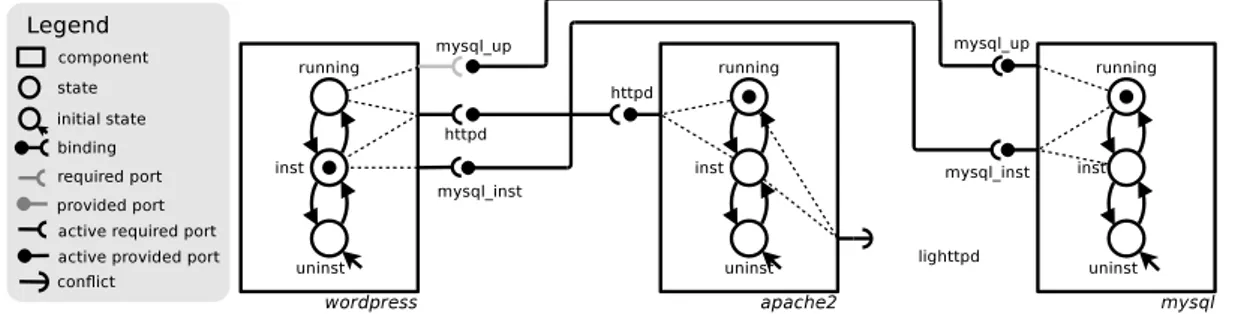
In Aeolus a component is described by a declarative specification of its behaviour by means of states and ports. This information is captured by so-called component types: every component belongs to a certain component type. The relevant internal states of components are represented by means of a finite state automaton 1 (see
Figure 5.1): depending on the current state, components activate provided and required ports, and get in conflict with ports provided by others (in Figure 5.1
active ports are black, while inactive ones are grey). Each port is identified by an interface name. Bindings can be established between provided and required ports with the same interface. Figure 5.1 shows the graphical representation of a typical deployment of the WordPress platform. WordPress requires a Web server providing httpd in order to be installed, and an active MySQL database server in order to be in production. In the example the chosen Web server is Apache2. Notice that Apache2
1It is important to notice that automata employed in Aeolus do not represent the internal behavior of components, but rather the effect on the component of an external deployment or reconfiguration actions.
Figure 5.1: Typical Wordpress/Apache/MySQL deployment, modeled in Aeolus.
is not co-installable with other Web servers, such as lighttpd. 2 This constraint is
depicted by means of a conflict arrow that is active in states inst and running of the Apache2 component.
At present time the Aeolus model is “flat” in the sense that all components live in a single “global” context, are mutually visible, and can connect to each other as long as their ports are compatible. To introduce a notion of hierarchy, different extensions to the original model, enriching it with membranes or boxes, have been envisaged but this part is still ongoing work.
Installing software on a single machine is a process that can already be automated using package managers: on Debian for instance, you only need to have an installed Apache server to be able to install WordPress. But bringing it in production requires to activate the associated service, which is more tricky and less automated: the system administrator will need to edit configuration files so that WordPress knows the network addresses of an accessible MySQL instance.
Services often need to be deployed on different machines to reduce the risk of failure or due to the limitations on the load they can bear. For example, system administrators might want to indicate that a MySQL instance can only support a certain number of WordPress instances. Symmetrically, a WordPress hosting service may want to expose a reverse web proxy / load balancer to the public and require
2Roughly specking, co-installable packages are packages that do not conflict. Refer to [57] for
Chapter 5. The original Aeolus model 37
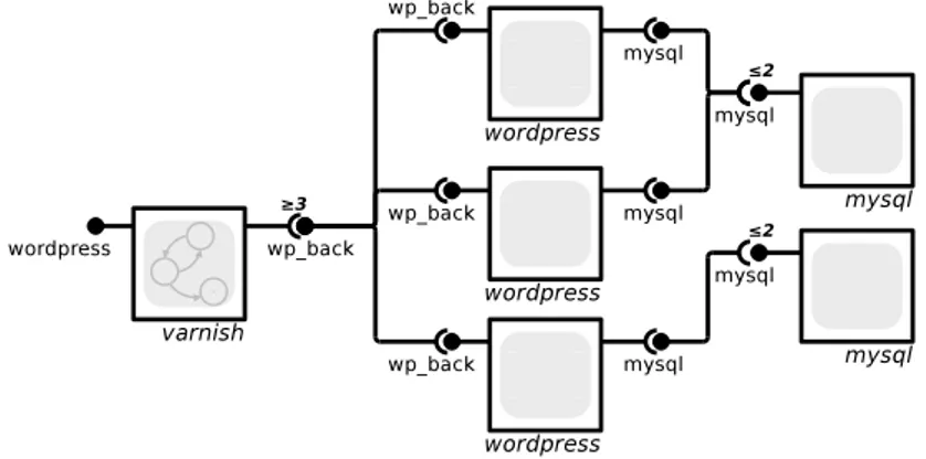
Figure 5.2: A graphical description of the model with redundancy and capacity constraints (internal sate machines and activation arcs omitted for simplicity).
to have a minimum number of distinct instances of WordPress available as its back-ends.
To model this kind of situations, Aeolus allows capacity information to be added on provided and required ports of each component: a number n on a provided port indicates that it can fulfill no more than n requirements, while a number n on a required port means that it needs to be connected to at least n provided ports from n different components. This information may then be employed by a planner to find an optimal replication of the components to satisfy a user requirement.
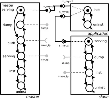
As an example, Figure5.2 shows the modeling of a WordPress hosting scenario where one wants to offer high availability hosting by putting the Varnish reverse proxy / load balancer in front of several WordPress instances, all connected to a shared replicated MySQL database 3. For a configuration to be correct, the model
requires that Varnish is connected to at least 3 (active and distinct) WordPress back-ends, and that each MySQL instance does not serve more than 2 clients.
As a particular case, a 0 constraint on a required port means that no provided port with the same name can be active at the same time; this can be effectively used to model conflicts between components.
Notation. We consider the following disjoint sets: I for interfaces and Z for components. We use N to denote strictly positive natural numbers, N∞ for N plus infinity, and N0 for
N plus 0.
Terminology. There is a distinction between the concept of interface and that of port : the latter being an “implementation” of the former. Throughout this work the two terms are sometimes used as synonyms, whenever there is no ambiguity in the given context.
In Aeolus components are modeled as finite state automata indicating the current state and the possible transitions. When a component changes its state, it can also change the ports that it requires from and provides to other components, thus adjusting its behaviour.
Definition 5.1 (Component type). The set Tf lat of component types of the Aeolus
model, ranged over by T1, T2, . . . contains 5-ple hQ, q0, T, P, Di where:
• Q is a finite set of states;
• q0 ∈ Q is the initial state and T ⊆ Q × Q is the set of transitions;
• P = hP, Ri, with P, R ⊆ I, is a pair composed of the set of provided and the set of required interfaces, respectively;
• D is a function from Q to 3-ple in (P 7→ N∞) × (R 7→ N0) × (R 7→ N0).
Given a state q ∈ Q, the three partial functions in D(q) indicate respectively the provided, weakly required, and strongly required ports that q activates. The functions associate to the active ports a numerical constraint indicating:
• for provided ports, the maximum number of bindings the port can satisfy,
• for required ports, the minimum number of required bindings to distinct com-ponents,
– if the number is 0, that indicates a conflict, meaning that there should be no other active port with the same name.
Chapter 5. The original Aeolus model 39
We assume as default constraints ∞ for provided ports (i.e. they can satisfy an unlimited amount of requires) and 1 for required (i.e. one provide is enough to satisfy the requirement). We also assume that the initial state q0 has no strong demands
(i.e. the third function of D(q0) is empty).
We now define configurations that describe systems composed by components and their bindings. A configuration, ranged over by C1, C2, . . ., is given by a set of
component types, a set of deployed components in some state, and a set of bindings. Formally:
Definition 5.2 (Configuration). A configuration C is a 4-ple hU, Z, S, Bi where:
• U ⊆ Tf lat is the universe of the available component types;
• Z ⊆ Z is the set of the currently deployed components;
• S is the component state description, i.e. a function that associates to com-ponents in Z a pair hT , qi where T ∈ U is a component type hQ, q0, T, P, Di,
and q ∈ Q is the current component state;
• B ⊆ I × Z × Z is the set of bindings, namely 3-ple composed by an interface, the resource that requires that interface, and the resource that provides it; we assume that the two components are distinct.
Notation. We write C[z] as a lookup operation that retrieves the pair hT , qi = S(z), where C = hU, Z, S, Bi. On such a pair we then use the postfix projection operators .type and .state to retrieve T and q, respectively. Similarly, given a component type hQ, q0, T, hP, Ri, Di, we use projections to (recursively) decompose it: .states, .init, and
.trans return the first three elements; .prov, .req return P and R; .Pmap(q), .Rwmap(q),
and .Rsmap(q) return the three elements of the D(q) tuple. When there is no ambiguity
we take the liberty to apply the component type projections to hT , qi pairs. Example: C[z].Rsmap(q) stands for the strongly required ports (and their arities) of component z in
configuration C when it is in state q.
We are now ready to formalize the notion of configuration correctness. We con-sider two distinct notions of correctness: weak and strong. According to the former,
only weak requirements are considered, while the latter also considers strong ones. Intuitively, weak correctness can be temporarily violated during the deployment of a new component configuration, but needs to be fulfilled at the end; strong correctness, on the other hand, shall never be violated.
Definition 5.3 (Correctness). Let us consider the configuration C = hU, Z, S, Bi. We write C |=req (z, r, n) to indicate that the required port of component z, with
interface r, and associated number n is satisfied. Formally, if n = 0 all components other than z cannot have an active provided port with interface r, namely for each z0 ∈ Z \ {z} such that C[z0] = hT0, q0i we have that r is not in the domain of
T0.P
map(q0). If n > 0 then the port is bound to at least n active ports, i.e. there exist
n distinct components z1, . . . , zn ∈ Z \ {z} such that for every 1 ≤ i ≤ n we have
that hr, z, zii ∈ B, C[zi] = hTi, qii and r is in the domain of Ti.Pmap(qi).
Similarly for provides, we write C |=prov (z, p, n) to indicate that the provided
port of resource z, with interface p, and associated number n is not bound to more than n active ports. Formally, there exist no m distinct components z1, . . . , zm ∈
Z \ {z}, with m > n, such that for every 1 ≤ i ≤ m we have that hp, zi, zi ∈ B,
S(zi) = hTi, qii and p is in the domain of Ti.Rwmap(qi) or Ti.Rsmap(qi).
The configuration C is correct if for each component z in Z, given S(z) = hT , qi with T = hQ, q0, T, P, Di and D(q) = hP, Rw, Rsi, we have that (p 7→ np) ∈ P
implies C |=prov (z, p, np), and (r 7→ nr) ∈ Rw implies C |=req (z, r, nr), and (r 7→
n0r) ∈ Rs implies C |=req(z, r, n0r).
Analogously we say that it is strong correct if only the strong requirements are considered: namely, we require (p 7→ np) ∈ P implies C |=prov (z, p, np) and (r 7→
nr) ∈ Rs implies C |=req(z, r, nr).
As our main interest is planning, we now formalize how configurations evolve from one state to another, by means of atomic actions.
Definition 5.4 (Actions). The set A contains the following actions:
Chapter 5. The original Aeolus model 41
• bind (r, z1, z2) where z1, z2 ∈ Z and r ∈ I;
• unbind (r, z1, z2) where z1, z2 ∈ Z and r ∈ I;
• new (z : T ) where z ∈ Z and T ∈ Tf lat;
• del (z) where z ∈ Z.
The execution of actions can now be formalized using a labeled transition systems on configurations, which uses actions as labels.
Definition 5.5 (Reconfigurations). Reconfigurations are denoted by transitions C −→α C0 meaning that the execution of α ∈ A on the configuration C produces a new
configuration C0. The transitions from a configuration C = hU, Z, S, Bi are defined as follows: C−−−−−−−−−−−−−→ hU, Z, SstateChange(z,q1,q2) 0, Bi if C[z].state = q1 and (q1, q2) ∈ C[z].trans and S0(z0) = hC[z].type, q2i if z0= z C[z0] otherwise C−−−−−−−−→ hU, Z, S, B ∪ hr, zbind (r,z1,z2) 1, z2ii if hr, z1, z2i 6∈ B
and r ∈ C[z1].req ∩ C[z2].prov
C unbind (r,z1,z2) −−−−−−−−−−→ hU, Z, S, B \ hr, z1, z2ii if hr, z1, z2i ∈ B C−−−−−−→ hU, Z ∪ {z}, Snew (z:T ) 0, Bi if z 6∈ Z, T ∈ U and S0(z0) = hT , T .initi if z0= z C[z0] otherwise C−−−−→ hU, Z \ {z}, Sdel (z) 0, B0i if S0(z0) = ⊥ if z0= z C[z0] otherwise and B0= {hr, z1, z2i ∈ B | z 6∈ {z1, z2}}
Notice that in the definition of the transitions there is no requirement on the reached configuration: the correctness of these configurations will be considered at the level of deployment run (Definition 5.7).
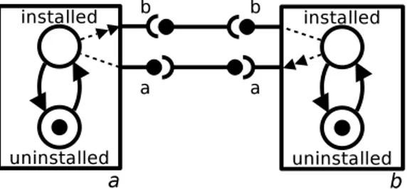
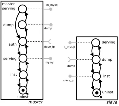
Also, we observe that there are configurations that cannot be reached through sequences of the actions we have introduced so far. In Figure 5.3, for instance, there is no way for package a and b to reach the installed state, as each pack-age require the other to be installed first. In practice, when confronted with such situations—that can be found for example in FOSS distributions in the presence of
Figure 5.3: On the need of a multiple state change action: how to install a and b?
Pre-Depend loops—current tools either perform all the state changes atomically, or abort deployment.
If one wants a planner to be able to propose reconfigurations containing such atomic transitions, one has to introduce the notion of multiple state change. 4
Definition 5.6 (Multiple state change). A multiple state change M = {stateChange(z1, q1
1, q21), · · · , stateChange(zl, ql1, q2l)} is a set of state change
actions on different component (i.e. zi 6= zj for every 1 ≤ i < j ≤ l). We use
hU, Z, S, Bi−→ hU, Z, SM 0, Bi to denote the effect of the simultaneous execution of the
state changes in M: formally, hU, Z, S, Bi stateChange(z
1,q1 1,q12) −−−−−−−−−−−−→ . . . stateChange(z l,ql 1,ql2) −−−−−−−−−−−−→ hU, Z, S0, Bi.
Notice that the order of execution of the state change actions does not matter as all the actions are executed on different components.
We can now define a deployment run, which is a sequence of actions that trans-form an initial configuration into a final correct one without violating strong cor-rectness along the way. A deployment run is the output we expect from a planner, when it is asked how to reach a desired target configuration.
4This kind of actions are part of the original model because one of its objectives was modeling uniformly both fine-grained components (such as packages) and coarse-grained ones (as services). If one focuses on modeling the latter, however, this kind of action can be ignored in favour of simplicity. This is the approach followed in this thesis, as we will explain in next chapter.
Chapter 5. The original Aeolus model 43
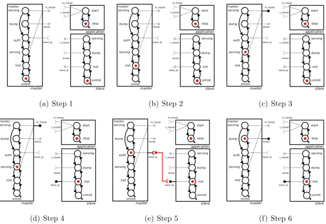
Definition 5.7 (Deployment run). A deployment run is a sequence α1. . . αm of
actions and multiple state changes such that there exist Ci such that C = C0, Cj−1 αj
−→ Cj for every j ∈ {1, . . . , m}, and the following conditions hold:
configuration correctness C0 and Cm are correct while, for every i ∈ {1, . . . , m −
1}, Ci is strong correct;
multi state change minimality if αj is a multiple state change then there
ex-ists no proper subset M ⊂ αj, or state change action α ∈ αj, and correct
configuration C0 such that Cj−1 M
−→ C0, or C j−1
α
−→ C0.
We now have all the ingredients to define the notion of achievability: given an universe of component types, we want to know whether it is possible to deploy at least one component of a given component type T in a given state q.
Definition 5.8 (Achievability problem). The achievability problem has as input an universe U of component types, a component type T , and a target state q. It returns as output true if there exists a deployment run α1. . . αm such that hU, ∅, ∅, ∅i
α1
−→ C1
α2
−→ · · · αm
−−→ Cm and Cm[z] = hT , qi, for some component z in Cm. Otherwise, it
returns false.
Remark 5.1. Notice that the restriction in this decision problem to one component in a given state is not limiting: one can easily encode any given final configuration by adding a dummy provided port enabled only by the desired final states and a dummy component with weak requirements on all such provided ports.
5.1
Decidability and complexity
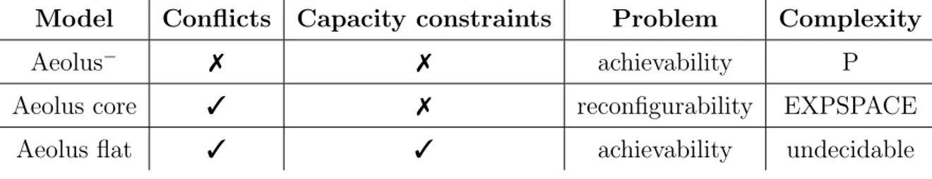
In this section we briefly summarize the formal results established for the achievabil-ity problem (Definition 5.8) cast in different variants of the original Aeolus model.
Table 5.1 gives an overview of the results proven in [30] and in [28]. The model considered is specified by listing in the second and third column if it allows to employ, respectively, conflicts and capacity constraints. The fourth column reports