ALMA MATER STUDIORUM
UNIVERSITA' DI BOLOGNA
FACOLTA' DI
Scienze Matematiche, Fisiche e Naturali
Corso di laurea magistrale in
Biologia Marina
Genetic structure and connectivity between populations of two
common Mediterranean sessile invertebrates.
Tesi di laurea in Ecologia applicata
Relatore
Presentata da
Prof. Marco Abbiati
Stefano Tassinari
Correlatore
Dott.ssa Federica Costantini
Dott.ssa Adriana Jacinta Villamor Martin Prat
II sessione
Index
page
Abstract 3
1.Introduction 5
1.1.Tools for the study of gene flow and connectivity 8
1.2.Theecosystem based management 10
1.3.The Mediterranean Sea 11
1.3.1. The central Mediterranean 14
1.4.Thetarget species 16
1.4.1.Halocynthia papillosa 16
1.4.2. Hexaplex trunculus 18
2. Aim of this work 20
3.Materials and methods 21
3.1.Sample collection 21
3.2.DNA extraction and amplification 22
3.3. Data analysis 23
3.3.1. Genetic diversity of populations 23
3.3.2. Population differentiation 24 3.3.3. Demographic analysis 25 4.Results 28 4.1.Halocynthia papillosa 28 4.1.1.Genetic diversity 28 4.1.2.Population differentiation 29 4.1.3.Demographic analysis 32 4.2.Hexaplex trunculus 35 4.2.1.Genetic diversity 35 4.2.2.Population differentiation 37 4.2.3.Demographic analyses 40 5. Discussion 42
5.1.Barriers to gene flow 42
5.2.Influence of life history traits 45
5.3.Genetic structure and diversity 46
5.4.Influence of past history events 48
5.5.Multispecies approach 49
5.6.Management applications 49
6. Conclusions 51
7. References 52
Abstract
Population genetic and phylogeography of two common Mediterranean species were studied in 10 localities located on the coasts of Toscana, Puglia and Calabria. The aim of the study was to verify the extent of genetic breaks, in areas recognized as boundaries between Mediterranean biogeographic sectors. From about 100 sequences obtained from the mitochondrial Cytochrome Oxidase subunit I (COI) gene of Halocynthia papillosa and
Hexaplex trunculus genetic diversity, genetic structure at small and large distances and
demographic history of both specieswere analyzed. No evidences of genetic breaks were found for the two species in Toscana and Puglia. The genetic structure of H. trunculus evidences the extent of a barrier to gene flow localized in Calabria, which could be represented by the Siculo-Tunisian Strait and the Strait of Messina. The observed patterns showed similar level of gene flow at small distances in both species, although the two species have different larval ecology. These results suggest that other factors, such as currents, local dynamics and seasonal temperatures, influence the connectivity along the Italian peninsula. The geographic distribution of the haplotypes shows that H.
papillosacould represent a single genetic pool in expansion, whereas H. trunculus has two
distinct genetic pools in expansion. The demographic pattern of the two species suggests that Pleistocene sea level oscillations, in particular of the LGM, may have played a key role in shaping genetic structure of the two species. This knowledge provides basic information, useful for the definition of management plans, or for the design of a network of marine protected areas along the Italian peninsula.
1. Introduction
Recognizing biodiversity and biogeographical patterns, and how these relate to contemporary and past events is relevant to better predict the effects of future global environmental changes (Xavier & Van Soest 2012). In the last years, genetic diversity has been proved to be a crucial part of biodiversity and it‘s been demonstrated that can act as a good indicator of population fitness (Claudet et al., 2008). Gene flow may influence the genetic diversity by introducing new polymorphisms in a population, on which evolution can potentially act. This gain of variability into a population may also protect it from extinction (Demarchi et al., 2010; Pérez-Portela et al., 2010). Furthermore, the genetic structure of a species can indicate how related are populations and what is their level of connectivity. In the marine realm, connectivity was long time thought to have no restrictions. However, with the recent widespread use of molecular tools, has been seen that even in cases of well known and widely distributed species, patterns of connectivity are not so obvious, shaping intricate genetic networks and peculiar population structures (Schunter et al., 2011; Kim et al., 2012). For the majority of marine animals, it‘s possible to have a general idea of the dispersal capability of adults and larvae knowing the larval phase duration and their ability to move actively in the water column, or to be passively transported by currents and eddies (Bertness, 2001). However, direct observations on larval dispersal are scarce and difficult. Many works, in fact, infer the dispersal potential only by larval period measures on laboratory experiments and not with direct observations of larvae movements in the water column (Ayre et al., 1997).
An indirect way of studying connectivity is gene flow: it is known that the occurrence of an allele in populations distributed in geographic locations can be an evidence of gene flow between populations (Carvalho, 1998). Thus, gene flow can be inferred from spatial distribution of genetic markers by several statistical approaches (Kelly et al., 2010; Avise, 2004). The study of population connectivity using genetic tools has greatly increased in the last 30 years; nevertheless our understanding of these processes is still largely underdeveloped (Bertness, 2001). These patterns of connectivity, in fact, are related to a large number of physical factors and to specific physiological and ecological traits, which might affect
According with the physiological factors, gene flow between populations can be promoted principally by migration and dispersion of both larvae and adults (Bahri-Sfar et al., 2000). Species that have pelagic adults have the potential to move widely throughout the oceans and face few barriers to dispersal (Horne et al., 2008). Most marine benthic organisms have a biphasic life cycle with sedentary adults and dispersing gametes or larvae, which may be pelagic from few minutes to more than a year (Toonen et al., 2011). Planktotrophic larvae feed on particles and plankton found in the water column, and hence have the potential to move out of their point of release in the search of food (Durante & Sebens 1994). However, the majority of invertebrate larvae move into the water column like passive o semi-active particles (Barber et al., 2000). In fact, species with larvae that spend little time in the plankton should be rare at larger distances from their original habitat showing a low dispersal potential, whereas larvae spending longer periods in the water column should be able to enter on the principal marine currents, implementing their dispersal potential (Durante & Sebens 1994). An example of these last is the benthic stomatopod Haptosquilla pulchella, with a 4-6 week planktonic larval period, having a dispersal potential estimated around 600 km (Barber et al., 2000). On the other hand, some ascidian species, with a planktonic larval phase ranging from few minutes (colonial ascidians) to 24-36 hours (solitary ascidians), are observed only near to the point of larval release (Ayre et al., 2009; Lòpez-Legentil & Turon, 2006). However, it‘s important to note that some species with high larval dispersal have a strong population structure, whereas some others with a priori low larval dispersal capacity can show a little genetic structure and hence high gene flow between distant populations. These unexpected dispersal patterns are due to numerous physical, hydrological and historical factors, that may greatly shape connectivity patterns (Hart & Marko, 2010).
The most important physical factor that might modify connectivity in the marine realm is the currents regime, mainly defined by its direction and velocity. Other secondary factors can be listed as the extent of land masses and the salinity and isothermal gradients (Borrero-Pèrez et al., 2011; Jackson, 1986). The water current regimes at several scales, from the largest general circulation to the smallest local eddies, are capable to modify dramatically the connection between nearby areas. Big general circulations, as recorded for the sea cucumber Holothuria
mammata across the Almerìa-Oran front, may negatively influence the connectivity
larval duration of H. mammata, but it is considered to be a broadcast spawner, having a relatively long planktotrophic larval stage of 13–22 days as has been recorded for other Holothurian species.The restricted gene flow evidenced between the Atlantic and Mediterranean populations is presumably due to the Almerìan-Oran front, in the convergence of Atlantic and Mediterranean water masses (Borrero-Pèrez et al., 2011). Moreover, current regimes at smaller scales may affect the distribution of population as has been shown for the Indonesian mantis shrimps, whose connectivity between nearby populations (distance range of 1,500 km) is very low due to the strong currents crossing the Indian Ocean (Barber et al., 2000).
On the contrary, some species with hypothetical low dispersal capacity are homogeneous between distant populations, as described for the Mediterranean bath sponge Spongia officinalis (Dailianis et al., 2011). However the larval time stage is unknown for this species and, as for some others sponges, it has been hypothesized to be relatively short with the settlement phase close to parental substrata. In spite of this, the S. officinalis populations analysed at 11 locations along the Eastern Mediterranean, Western Mediterranean and the Strait of Gibraltar, appeared to be genetically differentiated between the three basins, but homogenous within each basin (Dailianis et al., 2011). The reduced genetic structure of S. officinalis inside Mediterranean sectors, although the inferred low dispersal capacity, may be due to the current regimes of the basins (Dailianis et al., 2011). At the same time, general currents can be modified in local scales by coastal morphology. Near the coast, the currents are modified in very unpredictable ways by the coastal morphology, and this represents the main problem when trying to predict gene flow in coastal or shallow water species (Bianchi, 2007).
The isothermal regime of the seas, both superficial and deep, is another important factor which may modify the connectivity pattern of the species. Many Mediterranean recognized barriers are represented just by the isotherms following annual seasons (Brasseur et al., 1996). The surface isotherms divide the Mediterranean Sea in sectors which can influence the distribution of species (Brasseur et al., 1996). As it will be shown later, the February 15 C° surface isotherm on the Strait of Sicily may represent a point of break for species distribution at both sides of the strait, while the February 14 C° surface isotherm appear to be related to the differentiation between the Ionian and the Adriatic Seas
the case of the gastropods Charonia spp, represented by C. lampas lampas in the western basin and by C. tritonis variegata in the Eastern basin (Russo et al., 1990). However, not only present day processes affect the connectivity between populations in the marine realm. Current biodiversity patterns reflect the interplay between both contemporary and historical processes, which can generate vicariance or differentiation processes by long time physical separation (Huntley & Birks 1983). The most important historical events causing successive vicariance processes are glaciations, during which the sea level decreased, followed by interglacial periods, during which the sea level raises again reconnecting neighboring basins (Carstens et al., 2009). After the reunification of the basins, the vicariance might have resulted in speciation (Boissin et al., 2011), but in some other cases this speciation process might not have been completed and populations can still interbreed, showing this events reflected in their DNA sequences (Stefanni & Thorley, 2003). This is the case, for instance, of the chaetognath Sagitta setosa in the Mediterranean Sea, which shows two distinct mitochondrial lineages, showing some historical vicariance event, but no full speciation, according to nuclear markers (Peijnenburg et al., 2006). All these historical events, together with life history traits, contribute to delineate the actual distribution and differentiation of species (Ayre et al., 2009).
Understanding which factors affect the current genetic structure of marine species and if this pattern is determined by geographic distance, currents, or by past history events, is among the most crucial question in current marine research (Hart & Marko, 2010).
1.1.Tools for the study of gene flow and connectivity
In the last 20 years, the study of DNA sequences has provided a powerful tool to investigate the relationships between extant populations, giving valuable information on its current gene flow by means of highly variable markers (microsatellite, nuclear DNA), as well as information on past history events when analyzing conserved markers (mtDNA, allozyme) (Templeton et al.,1995; Yoder & Yang, 2000).
Phylogeography is the field of molecular ecology that investigates the geographical distribution of genetic lineages within species and studies the factors that shape their observed genetic architecture (Yoder & Yang, 2000).
Phylogeographic studies are usually aimed to address large-scale evolutionary patterns, related to biogeographic barriers (Rocha et al., 2007). It can also study a group of species across the same distribution area, in order to identify congruent patterns of genetic lineage distributions and hence indicate areas conforming evolutionary significant units (Rocha et al., 2007). In this kind of stu dies, conserved sequences are necessary. Conserved DNA areas usually codify for vital proteins, and hence, have a slow mutation rate. Moreover, these kind of studies need DNA sequences with relative constant mutation rates, which is inversely proportional to DNA gene function. For that reason, conserved and constant sequences should be preferred for phylogeographical studies (Hellberg & Vacquier, 1999).
Population genetics focus on current connectivity patterns at large and small spatial scales (Kelly e Palumbi, 2010). Population genetics is based on direct observation of allele or haplotype geographic distribution and mutation, making use of allele/haplotype identity and the relationship among them to infer the level of gene flow between populations and their subdivisions at small spatial scales (Carvalho, 1998). A central problem in population genetics is detecting fine scale population subdivision, created by current gene flow (Kelly e Palumbi, 2010). In the case of population subdivision, the accuracy of the parameters might be small when based only on a few individuals or when the migration rate is small (Ayre et al., 1997). Moreover, if the study is not repeated in time, might be difficult to verify whether the pattern observed is restricted in space and time or general (Carvalho, 1998). In population genetics studies, in contrast to phylogeographyc studies, highly variable molecular markers are used. These markers should have a high mutation rate, and usually are found in non-coding regions, so they are useful to detect small-scale genetic differences in small, subdivided populations (Peijnenburg et al., 2006).
Different mitochondrial markers offer a good variability of mutation rate (Emerson et al., 2001). For example, in human mitochondrial DNA some parts which are not involved in coding, evolve faster than protein-coding regions (Emerson et al., 2001). The mitochondrial Cytochrome c Oxidase subunit I (COI) gene appears to be among the most conserved protein-coding genes in the mitochondrial genome (mtDNA) of animals. The mtDNA is transmitted predominantly through maternal lineages in most species and although physical recombination does occur; it is unusual or rare in many taxa (Avise, 2004). For
estimates of ―matriarchal phylogeny‖ (Avise, 2004). At the same time, the COI gene offers a good level of genetic variation in the third position of each codon, position that does not involve change in the aminoacid coded. This properties make the COI gene suitable for analyses at different spatial scales, from phylogenetic to population genetic analyses, as it can retain the signature of both past and present demographic events of populations and species (Pérez-Portela et al., 2010).
1.2.The Ecosystem based management
Understanding patterns of connectivity through gene flow has several practical applications such as, for instance, the identification of evolutionary units or the identification of different stocks of commercial species. It is therefore a powerful tool to make proper decisions about sustainable exploitation (Lòpez-Legentil & Turon, 2006). The implementation of conservational studies is receiving increasing attention, especially in the sea, given the recent emphasis in the Ecosystem-Based-Management (EBM) (Rocklin et al., 2011). The EBM can be defined as an integrated approach that considers the entire ecosystem, including its interactions as well as the cumulative impacts of all human activities (Botsford et al., 2009). To properly enforce EBM, it is mandatory to understand the patterns of distribution and connectivity of the species, from the largest to the smallest spatial scales, in order to recognize and preserve the relevant biodiversity units present in a specific habitat (Kalkan et al., 2011; Kelly et al., 2010). In that sense, it is known that a certain species distributed in many small isolated populations, is less capable to recover against any kind of natural or anthropogenic disturbance. This is true in terms of population size (number of individuals), as well as in terms of genetic diversity (Claudet et al., 2008). The genetic diversity at the population‘s level is given by the level of polymorphism and heterozygosity, which might work as a proxy of the health state or fitness of populations as biodiversity units (Botsford et al., 2009).
The most important application of an EBM is the correct implementation of Marine Protected Areas (MPAs). MPAs are especially protected zones that respond to a series of conservational plans assisted by management and economical rules (Perry et al., 2010). One of the first Mediterranean MPAs was created inside the Bonifacio Strait (Corsica) during the 1980s, responding to a decline of commercial species stocks and biodiversity (Rocklin et al., 2011). Since then, biological, ecological and genetics studies have shown that effective MPAs also serve to
promote both effective species protection as well as spill-over to non-protected areas, benefitting also fisheries (Rocha et al., 2007). Thus, the positioning of those areas is critical, and their success is maximized when guided by accurate information about the organism‘s dispersal potential, the patterns of connectivity among populations and the knowledge of biodiversity units (Bird et al., 2007). Molecular tools can give information not only on the connectivity between populations, but also can help to infer the optimal size of a protected area as has been seen in several instances (Rocklin et al., 2011). Molecular tools can detect the existence of different genetic pools, suggesting the most effective protection strategy, and suggesting for instance, the implementation of several linked MPAs, rather than a bigger one (Claudet et al. 2008).
1.3.The Mediterranean Sea
The Mediterranean Sea is a fully enclosed sea, except for a small connection with the Atlantic Ocean, the strait of Gibraltar, and recently with the subtropical Red Sea by the Canal of Suez. This basin is the largest (2,969,000 km2) and deepest (average 1,460 m, maximum 5,267 m) enclosed sea, considered unique in the world for these features, but also for its peculiar hydrographic conditions, currents, temperature and salinity, which create a sharp gradient of conditions from West to East (Zulliger et al., 2009). In the Mediterranean Sea the evaporation is higher in its eastern half, causing the water level to decrease and salinity to increase from west to east. The resulting pressure gradient pushes cool, low-salinity water from the Atlantic across the Mediterranean Sea (Rizzo et al., 2009). The eastern region of the Mediterranean Sea is more oligotrophic than the western. Considering the whole Mediterranean basin the range of productivity decreases from north to south and west to east and is inversely related to the increase in temperature and salinity (Hamad et al., 2005).
The biodiversity of the Mediterranean Sea comprises approximately 17,000 species reported in the literature, among which at least 26% are prokaryotic and eukaryotic marine microbes. More than 8500 species are macro organisms, representing between 4% and 8% of the world‘s marine biodiversity (Coll et al., 2010). The main events structuring Mediterranean biodiversity pattern were the Atlantic flow of northern species during interglacial sea level rise, after ‗Messinian
Red sea after the recent opening of the Suez Canal (Boissin et al., 2011). Other recent climate change phenomena affect the oceanographic structure and biodiversity of the Mediterranean, among which tropicalization processes driven by global warming are the most evident (Bianchi & Morri, 2003).
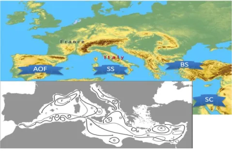
All the physical, historical and environmental factors, together with recent genetic data along the basin, have permitted to define three main physical breaks which have been found to act as effective barriers to gene flow: the Almeria-Oran Front (AOF); the Bosphorous Strait, and the Strait of Sicily (Figure 1)(Quesada et al., 1995; Duran et al., 2004; Luttikhuizen et al., 2008).
The AOF is an oceanographic front exhibiting a pronounced step of temperature (1.4 °C) and salinity (2 ppt) gradient, over a distance of 2 km with an average water current speed of 40 cm/s. It flows south/eastward from the Spanish coast to the coast of North Africa (Tintore et al. 1988),and forms a genetic break for many sessile and pelagic species, as the mollusk Mytilus galloprovincialis (Quesada et al., 1995), the sea urchin Paracentrotus lividus (Duran et al., 2004), the chaetognat Sagitta setosa (Peijnenburg et al., 2006), as well as for many fish and algae species (Coll et al., 2010).
The Bosphorus Strait is a well defined barrier for many species, due to its particular characteristics: During the interglacial period of the Middle Pleistocene, the Mediterranean waters entered in to the Black Sea driving an invasion of Mediterranean fauna, which is believed to have destroyed most part of the Black Sea fauna (Nikula & Väinölä, 2003). Nowadays there is a mutual exchange of water among the two seas: the Mediterranean Sea flows through the Bosphorus Strait depleting itself of oxygen, whereas the Black Sea low-salinity waters flow in to the Aegean Sea, with similar characteristics, supporting the larval flow between the two basins (Nikula & Väinölä, 2003; Kalkan et al., 2011).
Figure 1: Geographical position of the main Mediterranean physical breaks that act as effective
barriers to gene flow:AOF, Almerìa-Oran Front; SS, Strait of Sicily; SC, Suez Canal; BS, the Bosphorous Strait. In grey is shown the map of the main Mediterranean superficial fronts and currents (Bianchi, 2007).
In the central Mediterranean is located the Strait of Sicily, the area where the west and east side of the Mediterranean Sea are separated by a sharp reduction of depth and change in shallow currents (Stefanni & Thorley, 2003). In this area western currents flow on the clockwise direction, whereas Eastern currents flow on the contrary way, further complicated by small scale eddies and jets (Hamad et al., 2005). Moreover the Eastern basin is starved of phosphorous and is oligotrophic, enhancing the differences with the Western Mediterranean basin and strengthening this biogeographical break, described for many species (Krom et al., 2005). Many authors define the Strait of Sicily as the differentiation point of the paleo-biogeographical history of the Mediterranean Sea (Pancucci et al., 1999). In fact, the western basin shows a larger similarity with the Atlantic Ocean, hosting a higher number of cold-temperate species, while the eastern basin shows a large number of subtropical species (Bianchi & Morri, 2000). The Strait of Sicily represents a barrier to dispersal for many species, but also their meeting point. The presence, for instance, of the boreal-temperate species Golfingia margaritacea can indicate the prevalence, in that region, of colder water masses, whereas thermophilic species, such as Phascolion convestium and Aspidosiphon elegans, have been proposed as Lessepsian migrants (Tintore et al. 1988).
1.3.1.The central Mediterranean
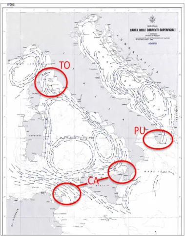
It is interesting to note that most of Mediterranean fronts and basins are influenced by the biodiversity and connectivity of its central area, where the Italian peninsula is located. As already recognized by Astraldi et al., (1999) and Bianchi, (2007), the Italian coasts, as the Mediterranean Sea, seem to be divided in numerous sectors considering currents, isotherms and coastal morphology (e.g. land masses, bathymetric changes, islands) (Figures 2 and 3). The Tyrrhenian biodiversity is influenced by the western/central Mediterranean basin, where the Islands of Sardinia and Corsica represent the main geographical break points. The Sardinia channel (large about 1900 m) represents the main way for Atlantic-western Mediterranean flow into Tyrrhenian Sea (Astraldi et al., 1999). On the Tyrrhenian Sea it is recognized another break, splitting the southern and northern Tyrrhenian Sea (the Gulf of Lion and the Ligurian Sea) (Bianchi, 2007). This area, corresponding to the Toscana archipelago represents a break, where the larval flow might be modified as currents split in two different directions (Figure 3). Furthermore, the coastal morphology of the archipelago with its bathymetric oscillations can greatly modify larval dispersion (Fredj & Giaccone, 1995).
The Adriatic/Ionian subdivision is not so clearlydefined by shallow currents. The Ionian currents (counterclockwise) seem to not meet the western Mediterranean basin (clockwise) and the Adriatic ones (Figures 1 and 3). For most authors, the genetic differences detected in some species among the Adriatic and the others eastern basins are due not to a contemporary break, but rather to ancient migrations of the species from south eastern regions to northern western and north eastern regions (Stefanni & Thorley, 2003). The pattern of Adriatic Sea currents that flow through the Ionian Sea and other eastern basins are not well explained in literature, making difficult any description of whole Ionian Sea currents (Millot, 1992). Moreover, the February isotherm of the southeastern basin of the Mediterranean Sea changes inside the Ionian basin, dividing isotherm of Calabria coast by Puglia coast. This may represent a physical break (Figure 2) (Millot, 1992).
In the present thesis, taking into account the oceanographical and historical characteristics of the Mediterranean Sea, we identified three hypothetical barriers to gene flow located around the Italian peninsula: Toscana, corresponding with the southern/northern Tyrrhenian division, Puglia, corresponding with the Adriatic/Ionian division, and Calabria, corresponding with the Tyrrhenian/Ionian
division (Figure 3). This third area is particularly interesting since it has been suggested as the major boundary between Eastern and Western Mediterranean.
Figure 2: Surface isotherms of February of the Mediterranean Sea (climatological means from the
historical data set 1906–1995). The 14 °C (red circle) and the 15°C (green circle) ‗divides‘ are highlighted by a thicker tract. Modified after MEDATLAS (Brasseur et al., 1996).
Figure 3: Map of superficial currents along the Italian coasts on
August/September (Istituto Idrografico della Marina, Genova 1982). The red circles represent the location of the hypothetical break: TO, Toscana ; CA, Calabria; PU, Puglia.
1.4.Thetarget species
The common assumption of past connectivity studies was that a single representative species could be used as a proxy to estimate dispersal among marine communities (Bird et al., 2007). During the last few years, it has been recognized that single-species studies on genetic connectivity were often contradictory considering the recognized barriers (Toonen et al., 2011; Bianchi 2007). Even among closely related species with similar ecology, life histories, and geographic ranges, the corresponding patterns of connectivity can be very different. In other cases species with highly divergent biology can have similar patterns of connectivity (Toonen et al., 2011). Such variability appears to be the rule rather than the exception, and has led to the necessity of multispecies comparisons.
Here, two widely distributed Mediterranean species living on rocky reefs, in the subtidal zone from 0 m to 200 m depth (Hofrichter, 2004; Bertness, 2001) were considered a two species study approach. The target species we have selected share some ecological characteristics as the geographic distribution, the bathimetric range and rocky substrata but they have some important differences as the reproduction seasonality and the adult mobility (H. papillosa is completely sessile where H.
trunculus is able to make slow movements) (Šantić et al., 2010; Lahbib et al.,
2010).
1.4.1.Halocynthia papillosa
Halocynthia papillosa (Figure 4) is an endemic Mediterranean ascidian of the
order Stolidobranchiata, family Pyuridae. It is one of the most common solitary species on the rocky bottoms of the Mediterranean Sea (Šantić et al., 2010).H.
papillosa is a non selective filter feeder, able to capture particles from 0.5 to 100
µm, with high retention efficiency for particles larger than 0.6 µm (Ribes et al., 1998).
Figure 4: Halocynthia papillosa on its habitat
Figure 5: oral pore of H. papillosa(http//www.commons.
wikimedia.org).
As most sessile suspension feeder ascidians, these organisms are dependent on the surrounding water, which provides them with their resources (Ribes et al., 1998). Therefore, this species prefers the habitats exposed to intense water currents (Santic et al., 2010). Thus, the largest number of individuals of this species can be found on exposed habitats as protruding land masses in areas with high water flow and nutrient content (Ribes et al., 1998). This species is also considered a good indicator of water quality, due to its capacity of concentrating toxic elements in their tissues, such as heavy metals and hydrocarbons (Tarjuelo et al., 2001).
H. papillosa is a hermaphroditic species and broadcast spawner, with external
fertilization that reproduces once per year in late summer. The chordate larvae are smaller than 500 µm of length and are lecithotrophic (Figure 6) (Šantić et al. 2010). The pelagic larval period of this species is not known, but for some others solitary ascidians it is thought between 12-24 hours, with a pre-competent period and prolonged metamorphosis of up to one week (Tarjuelo & Turon, 2004). H.
papillosa is thought to have a relative high dispersal ability (Zeng et al., 2006). In
fact, in a recent work Kim et al., (2012), studying the sister species Halocynthia
roretzi, have shown that these species may have a larval period of up to two weeks.
However, it has also been suggested that this larvae may use their swimming ability to stay close to the substrata of origin in search of appropriate settlement cues (Graham & Sebens, 1996).
Figure 6: Chordate Ascidiacean larva(http//etc.usf.edu.it).
1.4.2. Hexaplex trunculus
Hexaplex trunculus(also known as banded dye-murex, Figure 7) is one of the
most common gastropods of the Mediterranean Sea and Atlantic bottoms. It is a medium-sized species of the family Muricidae, living principally on hard substrata but recorded also on soft bottoms (Zarai et al., 2011).
Figure 7: Hexaplex trunculus (http//www.commons. wikimedia.org).
While during the Roman Empire this species was exploited for its purple dye, nowadays it is also a commercially exploited species, mainly for human consumption, thanks to its nutritive properties, and its potential to replace some overharvested fishes and mollusc species (Zarai et al., 2011). For this reason, during the lasts years H. trunculus has been widely studied in order to describe its reproductive cycle, nutritive properties, and its response to pollution on coastal
habitats (Lahbib et al., 2010). In fact, some works evidenced that the shell and the body of H. trunculus can incorporate some pollutants suspended in the water column and this can constitute a problem for human consumption. Moreover, these pollutants also influence the body size and the reproductive cycle of this species, diminishing the number of propagules production (Abidli et al., 2012).
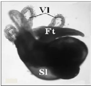
The banded murex H. trunculus, like most neogastropods, is gonochoric with internal fertilization (Fretter & Graham, 1994). The internal fertilization is performed following copulation and spawning of eggs within egg capsules. The incubation lasts 7 weeks, ending with the release of free juveniles (Figure 8). The time of gamete release is the same for male and female (from April to June) and seems to vary depending on habitat characteristics (currents and temperature oscillations) (Lahbib et al., 2010). Juveniles spend between 12 and 24 h searching for a suitable settlement surface (Lahbib et al., 2010).
Figure 8:hatched veliger juvenile of H. trunculus (Lahbib et
2. Aim of this work
The purpose of the present thesis is to verify the presence of barriers to gene flow generating discontinuities in the distribution of genetic diversity in two shallow rocky benthonic invertebrates. This main goal can be subdivided in several specific objectives. -To evaluate the effect of three potential barriers to gene flow located along the Italian coasts on connectivity patterns of two shallow rocky benthos species.
-As the two species studied Halocynthia papillosa and Hexaplex trunculus present contrasting reproductive modes and pelagic larval dispersal capacity, following the same sampling design for both species will allow to evaluate how life history traits can affect the population‘s genetic structure, its connectivity at several spatial scales, and how potential barriers to gene flow affects them.
-To understand large-scale genetic structure and connectivity around the Italian peninsula. Analyzing genetic differentiation among the three studied regions will give new information on phylogeographical patterns, and provide valuable data about genetic pools.
-By means of demographic studies we aim to understand how past history events affected the current genetic structure of the two species in the whole study area.
The number of species might be limited but it is useful to investigate the common connectivity patterns in the central Mediterranean Sea system along the Italian Peninsula. The importance, however, of past events genetic signal can be useful to improve our knowledge of genetic distributions during years and make inferences about resilience of the species and their response to future changes.
The results of this study, combined with the literature and with data collected in future studies, may also help to better implement an integrated and more comprehensive management and conservation plans, as for example the institution of marine protected areas (MPAs).
3.Materials and methods
3.1.Sample collection
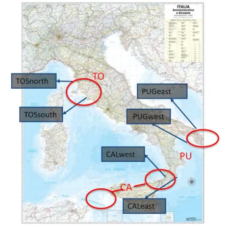
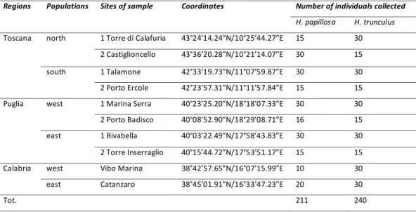
Samples of Halocynthia papillosa and Hexaplex trunculus were collected between July 2011 and June 2012 by scuba diving from 5 to 20 m of depth from Tuscany, Puglia and Calabria (Figure 9). The sampling design was as it follows: in each of the three studied regions one population from each side of the hypothesized barrier were considered on the analyses, but for Toscana and Puglia at each side we sampled on two sites (Table 1). These two populations were about 100 km apart (Figure 9; Table 1). In each sampling site at least 30 individuals of each species were collected (Table 1). Whole individuals of both species were sampled, given that underwater dissection of a piece of tissue was difficult and, in the case of H.
papillosa, did not avoid the death of the animal. Samples were immediately
preserved in ethanol 80% and stored at +4 C° until processed.
Figure 9: Map of the sample sites: TOSnorth, Toscana north;
TOSsouth, Toscana south; CALwest, Calabria west; CALeast, Calabria East; PUGwest, Puglia west; PUGeast, Puglia East. The red circles represent the location of the hypothetical break: TO, Toscana; CA, Calabria; PU, Puglia.(http//www.Google Chrome images.it).
Table 1: Regions, areas, sites, coordinates and number of individual collected of both species
Regions Populations Sites of sample Coordinates Number of individuals collected
H. papillosa H. trunculus
Toscana north 1 Torre di Calafuria 43°24’14.24”N/10°25’44.27”E 15 30 2 Castiglioncello 43°36’20.28”N/10°21’14.07”E 30 15 south 1 Talamone 42°33’19.73”N/11°07’59.87”E 30 30 2 Porto Ercole 42°23’57.31”N/11°11’57.84”E 15 15 Puglia west 1 Marina Serra 40°23’25.20”N/18°18’07.33”E 30 30 2 Porto Badisco 40°08’52.90”N/18°29’08.71”E 16 15 east 1 Rivabella 40°03’22.49”N/17°58’43.83”E 30 30 2 Torre Inserraglio 40°15’44.72”N/17°53’51.17”E 15 15 Calabria west Vibo Marina 38°42’57.65”N/16°07’15.99”E 10 30 east Catanzaro 38°45’01.91”N/16°33’47.23”E 20 30
Tot. 211 240
3.2.DNA extraction and amplification
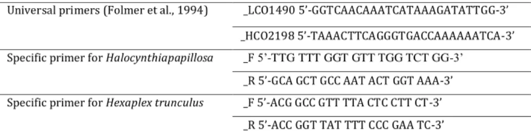
Total DNA was extracted using a REDExtract-N-AmpTMTissue PCR Kit protocol (SIGMA-ALDRICH). Total DNA was visualized in a 0,8% agarose gel, stained with Gelred (BIOTIUM) 1% after a 30 minutes electrophoresis at 120 V. The extraction product was diluted to 1:20 and 1:50 in ultrapure water (SIGMA) for better amplification success. A fragment of the mitochondrial COI gene was amplified with universal primers described in Folmer et al. (1994).As amplification was not consistent, from the first sequences obtained with the universal primers, specific primers were designed for each species with the software PRIMER vs.3.0 (http://www.fokker.wi.mit.edu/primer3/input.htm) (Table 2).
The PCR amplification reactions were performed in a 25 µL final volume consisting of: 2.5 µL of DNA template, 2.5 µL of buffer (PROMEGA), 2.5 µL of MgCl2 25 mM (PROMEGA), 2 µL of dNTPs 10 mM, 1.25 µL of each forward and
reverse specific primers 10 mM (MACROGEN), 12.8 µL of ultrapure water (SIGMA) and one unit (0.2 µL) of Taq polymerase enzyme (Invitrogen). PCR reaction was performed in a GeneAmp® PCR Sistem 2700 thermocycler (Applied Biosytems). The amplification conditions were as follows: an initial denaturation at 94 °C for 3 min followed by 30/35 cycles of 94 °C for 45 sec, 45 sec at a specific annealing temperature (46/50 °C C for H. trunculus and H papillosa respectively) and an extension at 72 °C for 90 sec. After a final extension of 5 min at 72 °C products were maintained at 4ºC. Products of amplification were visualized in a 1,5% agarose gel stained as previously described.
Table 2: Table of universal primers and primers sequences for H. papillosa and H. trunculus.
Universal primers (Folmer et al., 1994) _LCO1490 5’-GGTCAACAAATCATAAAGATATTGG-3’ _HCO2198 5’-TAAACTTCAGGGTGACCAAAAAATCA-3’ Specific primer for Halocynthiapapillosa _F 5‘-TTG TTT GGT GTT TGG TCT GG-3‘
_R 5’-GCA GCT GCC AAT ACT GGT AAA-3’ Specific primer for Hexaplex trunculus _F 5’-ACG GCC GTT TTA CTC CTT CT-3’
_R 5’-ACC GGT TAT TTT CCC GAA TC-3’
PCR products were sent to Macrogen Europe Inc. for purification and sequencing. Sequences were checked by eye and edited with ChromasPro vs1.5 (www.Technelysium.com.au/ChromasPro.htlm). Alignments were performed using MEGA 5 (Tamura et al 2011).
3.3.Data analysis
3.3.1.Genetic diversity of populations
Nucleotide diversity π, number of haplotypes h, haplotype diversity Hd, number (Np) and the percentage of private haplotypes (%Np) were calculated using
DnaSP v5.10 software (Rozas et al., 2003) for all populations at each side of the hypothetical barriers and for the three regions (Table 1). The number of private haplotypes gives a further indication of the diversity of a population (Kelly et al., 2010).
The relationships between haplotypes were represented in a haplotype network, performed with the software Network v4.6.1.0 (Fluxus Technology Ltd.).The Median-Joining network is implemented showing the differences between aligned sequences of one or more populations in a network of distance measures. The simplest way to obtain a distance measure between two sequences is to count the number of character differences and weight the character changes (Bandelt et al., 1999).It is based on improved Kruskal‘s (1956) algorithm, which lists triplets of sequences in increasing order of distance. The resulting network shows the sequences or individuals grouped together according to the haplotypes recognized and their relative distances (Bandelt et al., 1999). This type of network allows identifying haplotypes that are more frequent among a group of individuals, a location, populations that share haplotypes or not etc. The haplotype network gives,
good representation of population genetic structure and some indirect indications of actual population size (Hart & Marko, 2010).
3.3.2.Population differentiation
To study similarity between populations the Fst index between each pair of
populations was calculated. Fst can be interpreted as the proportion of genetic
variation distributed among and within subdivided populations and indirectly of the level of gene flow between populations (Beerli & Felsenstein 1999). Fst values
range between 0, indicating that populations are genetically identical, and 1, indicating that populations are differentiated according to the specific alleles. To better visualize the results of pairwise Fst values, we represented on a bidimensional
space the matrix of dissimilarity in a Multidimensional scaling representation (MDS), using the Primer software (Clarke & Ainsworth, 1993).
According to the results of pairwise Fst, we grouped populations in
homogeneous groups, where no significant genetic differentiation was detected. We analyzed the Molecular Variance of these groups, AMOVA, implemented in Arlequin software v3.5.1.2 (Excoffier & Lischer 2010). The Analysis of molecular variance assigns percentages of variability explained and a significance to the variability among groups, within populations inside the groups and within populations without grouping, giving information on the degree of homogeneity of the groups set and how differentiated are from each other.
Finally, the Isolation by distance model was tested with a Mantel test (Mantel, 1967) with 1000 permutation in Arlequin v3.5.1.2 (Excoffier & Lischer 2010). The Mantel test calculates the correlation between two matrices, one of them is the genetic distance as Fst/1-Fst and the other is the matrix of log-transformed
geographical distances between populations. The isolation by distance model predicts that genetic differentiation will be proportional to geographic distance. If Mantel test results not significant, no correlation between the two matrices exists, and hence it should be inferred that some factors other than distance are affecting the differentiation between populations.
Finally, with the software MIGRATE (Beerli & Felsenstein 1999), we inferred the approximate number of migrants between these three regions. MIGRATE uses a method to make a maximum-likelihood estimate of population parameters for
geographically subdivided populations, using gene frequency distribution and including on this method the Coalescent theory (Beerli & Felsenstein 1999).
3.3.3.Demographic analysis
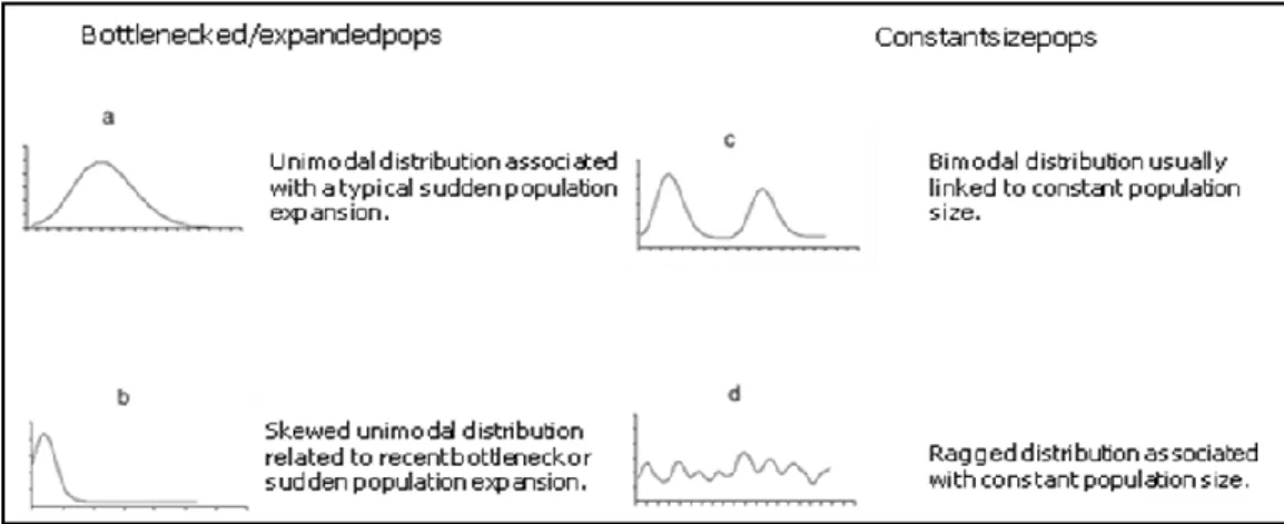
Demographic analyses allow to evaluate the changes on population size through time and infer information on the behavior of populations during past history events (Rogers & Harpending, 1992). It is known that changes in population size left signatures in DNA sequences as proportion of differences, so mismatch distribution analysis are calculated as the frequency of pairwise differences between haplotypes, which can be represented in a graph for better interpretation. The mismatch distribution method is based on the assumption that a rapid population expansion is plotted on the line graph like a peak, as there is a high frequency of individuals with small number of pairwise differences, whereas stable population size has a multimodal distribution of growths and declines (Figure 10) (Harpending, 1994). Mismatch distribution also allow the detection of subpopulations, different genetic pools that coexist in the same geographic area. In figure 10 are shown the most common types of mismatch distribution that populations can show.
Figure 10: Main types of mismatch distributions: (a) unimodal distribution associated with a typical sudden population
expansion; (b) skewed unimodal distribution related to recent bottleneck or sudden population expansion; (c) bimodal distribution usually linked to the presence of more than one genetic pool; (d) ragged distribution associated with constant population size (Patarnello et al.,2007).
For H. papillosa the mismatch distributions for the whole sequences and for the three regions were calculated, while for H. trunculus the mismatch distributions of the two groups found on Fst analyses.
initially for ecologically studies of populations‘ connectivity (Kimura, 1968). However, the neutrality theory applied to molecular ecology states that ―mutation substitutions on sequences are caused by random changes of selectively neutral marker under continued mutation pressure‖ (Kimura, 1991). Alleles at a given locus are selectively neutral, i.e. substituting one allele by another does not affect the fitness of an individual or of a population (Rosindell et al., 2011). Regarding a neutral marker, at large time scales it is notable that mutations would not affect in a large extent the resilience of populations in terms of genetic complexity. The molecular variability can be hence described as a function of neutral mutation rate and effective population size (Avise, 2004).
The Tajima‘s D relates the number of segregating sites and the average number of nucleotide differences estimated with pairwise sequences comparison (Tajima, 1989), while Fu‘s test compares the number of slightly different alleles (typical of expanding populations) with the number of alleles statistically expected in a expanding population (Fu, 1997). Significant negative D and Fs values mean significant departures from mutation-drift equilibrium of populations and can be interpreted as signatures of population expansion. In the opposite, positive values can be interpreted as situations of constant size and in equilibrium populations (Patarnello et al., 2007).
The approximate time of expansion was calculated for those populations fitting the sudden expansion model with the Harpending (1992) equation:
Ƭ=2ût; û=2µk
Where t is the time expressed in generations and û is the per-generation probability of a sequence to have a mutation anywhere. The term û is given by the average number of nucleotide k of the COI amplified sequences and by the termµ, the mutation rate per nucleotide which changes according to different species. Although genes mutate at different rates according to their characteristics (mtDNA, nuclear DNA, allozymes), the common assumption that genes evolve with a nearly constant rate at long time scales is accepted (Hellberg & Vacquier, 1999). For an expanding population, knowing the mutation rate per nucleotide and the number of nucleotides of a sequence, is possible to calculate the time when the expansion began and relate it to a particular historical event (Rogers & Harpending, 1992). The general mutation rates applied for gastropods‘COI is 2.4% per million years
(Hellborg & Vacquier 1999). The mtDNA mutation rate of H. papillosa is not reported on literature but that ofH. roretzi is estimated in 2.86% per million years so it is possible that H. papillosa has the same (Kim et al., 2012).
4.Results
4.1.Halocynthia papillosa
4.1.1.Genetic diversity
A portion of 371bp of the COI gene was obtained from 113 individuals of
Halocynthia papillosa: 58 individuals from Toscana, 40 from Puglia, and 14
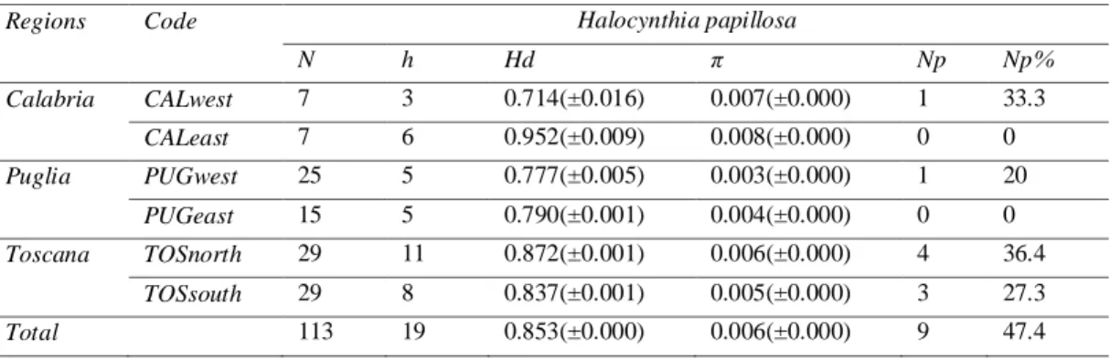
individuals from Calabria (Table 3). A total of 19 haplotypes were obtained, where 9 of them were private, 7 of which were found in Toscana populations (Table 3).
The haplotype diversity (Hd) and nucleotide diversity (π) detected for the whole data set of this species are, respectively, 0.853 and 0.006, similar to those found for each region independently (Table 3).
Table 3: Table of diversity index of H. papillosa:N, number of sequences; h, number of haplotypes; Hd, haplotype diversity± standard deviation; π, nucleotide diversity± standard deviation; Np, number of private haplotypes; Np%, percentage of private haplotypes. Code: TOSnorth, Toscana north; TOSsouth, Toscana south; CALwest, Calabria west; CALeast, Calabria east; PUGwest, Puglia west; PUGeast, Puglia east.
Regions Code Halocynthia papillosa
N h Hd π Np Np% Calabria CALwest 7 3 0.714(±0.016) 0.007(±0.000) 1 33.3 CALeast 7 6 0.952(±0.009) 0.008(±0.000) 0 0 Puglia PUGwest 25 5 0.777(±0.005) 0.003(±0.000) 1 20 PUGeast 15 5 0.790(±0.001) 0.004(±0.000) 0 0 Toscana TOSnorth 29 11 0.872(±0.001) 0.006(±0.000) 4 36.4 TOSsouth 29 8 0.837(±0.001) 0.005(±0.000) 3 27.3 Total 113 19 0.853(±0.000) 0.006(±0.000) 9 47.4
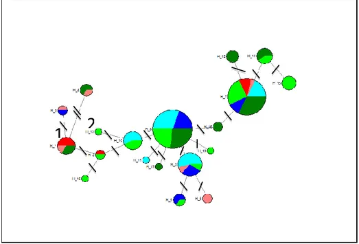
In the haplotype network, it is possible to see that the two more frequent haplotypes (H_7 and H_8) are common in Toscana populations which also present large number of low frequency and private haplotypes, closely linked to H_7 and H_8 (Figure 11). As already evidenced on Table 3, Toscana has more private haplotypes than Puglia (only one, H_11). The H_1 is more common in Calabria, which also shows other common haplotypes, as H_7 and H_3, less common as the H_4, H_5, H_2, and one single private haplotype, H_6 (Figure 11).
Figure 11: Haplotype network of Halocynthia papillosa. Colors represent the populations: TOSnorth,
light green; TOSsouth, dark green; CALwest, red; CALeast, pink; PUGwest, blue; PUGeast, light blue. Short black lines represent the number of mutations between the haplotypes. Two black lines with number 2 represent two mutation where one black line represent one mutation. The number 1 represents one mutation and the 2 number represents two mutations.
4.1.2.Population differentiation
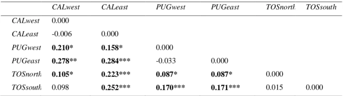
The pairwise Fst analyses do not show significant differentiation between
populations located at each side of the hypothesized barriers in any of the three regions (Table 4). Between regions, Fst values show small but significant
differences in all pairwise comparisons, except between TOSsouth (the south area of Toscana) and CALwest (the west area of Calabria) (Table 4). When pooling together populations of each region all three regions show significant differences between them, however Puglia seems to be more similar (in terms of Fst value) to
Toscana than Calabria (Table 5). The highest differences occur between Calabria and Toscana, with a differentiation value of 0.378 and P=0.000 (Table 5).
The pairwise differences between all the populations are represented in the multidimensional scaling (Figure 13), where populations belonging to the same region are closer together.
2
1
Table 4: Table of pairwise differences (Fst) between Halocynthia papillosa populations: TOSnorth, Toscana north; TOSsouth, Toscana south; CALwest, Calabria west; CALeast, Calabria east; PUGwest, Puglia west; PUGeast, Puglia east.
CALwestA CALeast PUGwest PUGeast TOSnorth TOSsouth
CALwest 0.000 CALeast -0.006 0.000 PUGwest 0.210* 0.158* 0.000 PUGeast 0.278** 0.284*** -0.033 0.000 TOSnorth 0.105* 0.223*** 0.087* 0.087* 0.000 TOSsouth 0.098 0.252*** 0.170*** 0.171*** 0.015 0.000 * = P< 0.05; **=P< 0.01; ***= P<0.000.
Table 5: Table of pairwise differences (Fst) of
Halocynthia papillosa regions when population
within regions are pooled together.
Calabria Puglia Toscana
Calabria 0.000
Puglia 0.341*** 0.000
Toscana 0.378*** 0.103*** 0.000 *=P< 0.05;**=P< 0.01; ***= P<0.000.
Figure 12: Multidimensional scaling (MDS) of the 6 populations of H. papillosa. Blue
According to the Fstvalues obtained, we run the AMOVA analyses with three
groups corresponding to the three regions (Table 6). The results show that most of the variability is due to differences within populations (94.72%, P=0.005 whereas the variability among groups explain only the 4.99% of the total variation (P=0.078).
Table 6: Table of AMOVA of all populations of H. papillosa.
Source of variation d.f. Sum of squares Variance components Percentage of variation P value Among groups 2 2.309 0.021 4.99 0.078 Among populations within groups 3 1.307 0.001 0.29 0.394 Within populations 107 44.127 0.412 94.72 0.005 Total 112 47.743 0.435 Significance when P< 0.05
For H. papillosa the Mantel test did not detected a significant correlation between pairwise differences among populations and geographic distance (P=0.16), indicating that the genetic differentiation detected between regions is not proportional to geographic distance, as expected following pairwise Fst values.
The MIGRATE results show a great effective population size on Toscana, with an average Θ value of 0.016. The most relevant migration rate seems to be from Calabria to Puglia (mean=629.7) whereas the opposite migration rates from Toscana and Puglia to Calabria are much lower (Figure 13-14). The migration rate from Calabria to Toscana is not symmetric and with a higher variance. Between Puglia and Toscana we also detect a not perfectly symmetric migration but relevant, with a mean of 604.3(Figure 13-14).
Figure 13a: H. papillosa migration rates of Bayesian Analyses Posterior Distributions. The black area
indicates the highest probabilities.
Figure 13b: H. papillosa migration rates of Bayesian Analyses Posterior Distributions. The black area
indicates the highest probabilities.
Figure14:H. papillosamigration rates of Bayesian Analyses Posterior Distributions.
4.1.3.Demographic analysis
The mismatch distribution of the whole data set of Halocynthia papillosa fits to a pattern of sudden expansion (goodness of fit=0.001P=0.770) (Figure 15). Because no significant differences were detected inside each region (Table 4), we only performed the mismatch distributions of each region separately (Figures 16-17-18).
Figure 15: Mismatch distribution of the whole data set of Halocynthia papillosa.
For the whole data set, Tajima‘s D test was positive and not significant (D=1.224; P=0.908), while Fu‘s was negative and highly significant (F=-17.458 P=0.000) (Table 7), indicating population expansion. The mismatch distributions of the regions fit to a pattern of sudden expansion model, with significant Fu‘s neutrality test (Figure 16-17-18 and Table 7). Tajima‘s D neutrality tests were not significant in any case (Table 7), but Fu‘s test has been suggested to be more powerful in detecting neutrality (Avise, 2004). As calculated with Harpending, (1992) equation, Halocynthia papillosa experienced a recent expansion, about 17700 years ago (µ=2.86/million years; 1 generation/year).
Table 7: Table of mismatch goodness of fit and neutrality tests of the three
regions. Significant values when P<0.05.
Regions Goodness of Fit Tajima’s D Fu’s Fs
Calabria 0.003(P=0.950) 0.171(P=0.591) -4.038(P=0.009) Puglia 0.001(P=0.690) -1.137(P=0.118) -6.632(P=0.001) Toscana 0.000(P=0.940) -0.832(P=0.234) -17.458(P=0.000) All seq. 0.001(P=0.770) 1.224(P=0.908) -7.100(P=0.010) 0,0 200,0 400,0 600,0 800,0 1000,0 1200,0 1400,0 1600,0 1800,0 0,0 2,0 4,0 6,0 8,0 10,0 Obs. Mod.freq. Pairwise differences Fr eq u en cies
Figure 16: Calabria mismatch distribution of H. papillosa.
Figure 17: Puglia mismatch distribution of H. papillosa.
0,0 2,0 4,0 6,0 8,0 10,0 12,0 0,0 5,0 10,0 15,0 Obs Mod.freq. Pairwise differences Fr eq u en cies 0,0 20,0 40,0 60,0 80,0 100,0 120,0 140,0 160,0 180,0 200,0 0,0 2,0 4,0 6,0 8,0 10,0 12,0 Obs Mod.freq. Pairwise differences Fr eq u en ci es
Figure 18: Toscana mismatch distribution of H. papillosa.
4.2.Hexaplex trunculus
4.2.1.Genetic diversity
Sequences of 523bp of the mitochondrial gene COI from 100 individuals of
Hexaplex trunculuswere obtained. The number of sequences (N) obtained by region
was more homogenous than in the case of H. papillosa: 36 sequences from Toscana, 37 from Puglia and 27 sequences from Calabria (Table 8).
Out of 27 haplotypes (h)9 of them were found only in Calabria, 8 in Puglia, and 5 in Toscana (Table 8). The haplotype diversity (Hd) of the whole data set is slightly lower than that seen in H. papillosa (0.753), and the same is true for each of the three regions (Table 8). The smallest values of Hdand π are found in Toscana, whereas the highest values are found in Calabria (Table 8).
0,0 50,0 100,0 150,0 200,0 250,0 300,0 350,0 400,0 450,0 0,0 5,0 10,0 Obs Mod.freq. Pairwise differences Fr eq u en ceis
Table 8: Table of genetic diversity index of H. trunculus:N, number of sequences; h, number of haplotypes; Hd, haplotype
diversity± standard deviation;π, nucleotide diversity± standard deviation; Np, number of private haplotypes; Np%, percentage of private haplotypes. Populations: TOSnorth, Toscana north; TOSsouth, Toscana south; CALwest, Calabria west; CALeast, Calabria east; PUGwest, Puglia western; PUGeast, Puglia east.
The haplotype network of Hexaplex trunculusshows two well distinct clades separated by 10 mutations, each one of them showing a clear star-like shape (Figure 20).The clade-A is characterized by one more common haplotype (H_3), one less common haplotype (H_7) and few other private haplotypes (Figure 19). The haplotypes of clade-A, are present only in Puglia (light and dark blue), Calabria east (pink) and in a single individual (H_27) of Calabria west (red). The clade-B seems to be more polymorphic and geographically widespread, with haplotypes present in all the populationsand in the three regions. The H_4 is the most common haplotype on the clade B and appears in Puglia, Calabria and Toscana (Figure 20). There is also an individual of Toscana north (H_16) linked with more than 18 mutation steps to haplotypes of Calabria individuals (Figure 19).
Regions Code Hexaplex trunculus
N h Hd π Np Np% Calabria CALwest 12 5 0.803(±0.006) 0.006(±0.000) 2 40 CALeast 15 9 0.848(±0.007) 0.012(±0.000) 7 77.7 Puglia PUwest 17 8 0.846(±0.003) 0.013(±0.000) 5 62.5 PUeast 20 6 0.763(±0.004) 0.011(±0.000) 3 50 Toscana TOSnorth 24 5 0.312(±0.010) 0.003(±0.000) 4 80 TOSsouth 12 2 0.167(±0.010) 0.000(±0.000) 1 50 Tot 100 27 0.753(±0.001) 0.013(±0.000) 22 81.5
Figure 19: Haplotype network of Hexaplex trunculus.Colours represent the populations:
TOSnorth, light green; TOSsouth, dark green; CALwest, red; CALeast, pink; PUGwest, blue; PUGeast, light blue. More than one mutation is signed with two black lines and numbers; one line is one mutation. Number 2 indicates two mutations, number 8 indicates eight mutations, number 10 indicates ten mutations and number 18 indicates eighteen mutations. The upper right clade is clade-A, the lower left clade is clade-B.
4.2.2.Population differentiation
The Fst values show no pairwise differences among the populations inside Puglia
and Toscana (Table 8). Inside Calabria, a sharp differentiation between the two populations was detected (Fst=0.531, P=0.000).Moreover, Toscana and Puglia are
significantly different (Table 8). The western population of Calabria (CALwest) shows small but significant differences with Toscana and larger differences with Puglia. The eastern Calabria population (CALeast) shows small differences with Puglia populations (Table 8).
The representation of these Fst values shows how populations inside Puglia and
Toscana are grouped together, whereas the two regions are highly distinct (Figure 20). It is also represented the large differentiation between the two populations of Calabria (Figure 20). It is also possible to recognize two clear groups that fit Fst
pairwise differences: one group, (Southern Group hereafter), formed by Puglia and Calabria east populations, and a second group (Northern Group hereafter) including Toscana and Calabria west populations.
Table 8: Table of pairwise differences of all populations of Hexaplex trunculus: TOSnorth, Toscana north area; TOSsouth,
Toscana south area; CALwest, Calabria west area; CALeast, Calabria east area; PUGwest, Puglia west area; PUGeast, Puglia east area.
CALwest CALeast PUGwest PUGeast TOSnorth TOSsouth
CALwest 0.000 CALeast 0.531*** 0.000 PUGwest 0.480*** 0.026 0.000 PUGeast 0.263*** 0.145* 0.032 0.000 TOSnorth 0.160*** 0.670*** 0.592*** 0.376*** 0.000 TOSsouth 0.222*** 0.664*** 0.581*** 0.347** -0.028 0.000
Signification of * at P< 0.05;**, P< 0.01; ***, highly significant at P=0.000.
Figure 20: MDS of pairwise Fst values between all populations of H. trunculus.The Northern Group includes down right side populations TOSnorth, TOSsouth and CALwest, and the Southern Group include upper left side populations, PUGwest, PUGeast and CALeast. Blue circles include the two groups found on Fst analyses.
The AMOVA analyses were conducted for the two groups detected according to Fst values, Southern Group and Northern Group. The highest variation is found
within populations (68.95%) and among groups (17.41%) however this last is not significant (Table 9). The Fstbetween the Southern Group and Northern Group is
Table 9: Table of AMOVA of the two groups of H. trunculus. The Northern Group is compost of Toscana and Calabria
west populations; the Southern Group is compost of Puglia and Calabria east populations.
Source of variation d.f. Sum of squares Variance components Percentage of variation P value Among groups 1 5.577 0.073 17.41 0.341 Among populations within groups 2 2.719 0.057 13.64 0.000 Within populations 93 27.106 0.291 68.95 0.000 Total 96 35.402 0.422 Significationat P< 0.05.
The low P value shown among groups (P=0,341), although the percentage of variation is evident (17,41%), is probably due to the fact that these two groups (Figure 21) do not correspond to the real segregation of individuals inside the two clades recognized on the haplotype network (Figure 19). For this we separated the individuals of Puglia and Calabria east belonging to the two clades and performed the AMOVA between the two clades (Table 10). In this case we did detect a significant percentage of variation explained among these two clades (42.14%, P=0.010). Fst value between clade-A and -B is highly significant (Fst=0.451;
P=0.000).
Table 10 AMOVA betweenthe two clades of H. trunculus. Clade-A and clade-B are described above and are shown on
haplotype network (Figure 19).
Source of variation d.f. Sum of squares Variance components Percentage of variation P value Among groups 1 9.623 0.20455 Va 42.14 0.010 Among populations within groups 7 4.388 0.03780 Vb 7.79 0.000 Within populations 88 21.390 0.24307 Vc 50.07 0.000 Total 96 35.402 0.48542 Signification at P< 0.05.
The Mantel test not showed significant correlation between the genetic diversity and geographic distance (P=0.05).