Control of matter wave tunneling in an optical lattice

(1)

Control of matter wave tunneling in an

optical lattice

Carlo Sias

Advisor:

Prof. Ennio Arimondo

Universit`a degli Studi di Pisa

Dipartimento di Fisica E. Fermi

Corso di Dottorato in Fisica Applicata

V Ciclo

(2)

(3)

Acknowledgements

When I arrived in Pisa four years ago I did not know almost anything about experiments with Bose-Einstein condensates. During my Ph.D. I had the opportunity to learn so many things on this subject, so that now I really want to acknowledge all the people that accompanied and helped me in this long way. I want to thank Prof. Ennio Arimondo, who allowed me to work in his laboratory and who encouraged me in working on such interesting topics. Oliver Morsch and Donatella Ciampini were for me as Virgilio and Beatrice for Dante, joining hands with me whenever the way was dark, and theoretical and experimental difficulties were overcoming me. Matteo Cris-tiani, Emmanuel Courtade, Hans Lignier, Yeshpal Singh, Sandro Wimberger, Alessandro Zenesini were not only my ”labmates” during these years: the many scientific discussions we had day by day in the laboratory, that have been fundamental for me to understand the physics we investigated, were joined by discussions about life, so that our relationships became real, won-derful friendships. The Pisa team was like a family for me. And a part of this family were Prof. Maria Allegrini, Prof. Francesco Fuso, Francesco Tantussi (Tupi), Enrico Andreoni and Nicola Puccini. With their help we managed to recover the experiment after the family drama, i.e., the fire that in 2005 occurred in our laboratory. As far as the work presented in this thesis is concerned, I acknowledge Prof. Martin Holthaus and Andr´e Eckardt for the enlightening discussions we had, especially during their visit in Pisa in 2007. I want also to thank Prof. Francesco De Martini, who encouraged me to move to Pisa to learn about experimental atomic physics.

Apart from the ”laboratory family”, I had another family in Pisa, made of all the friends I met during these years. Our common house was the flat I developed with Sascha and Angelo. Our common time was made of sharing the happiness and disgraces of our lives (quite often while drinking a beer). Thanks to all these friends, I will always remember my time in Pisa as one of the best in my life.

But apart from the ”laboratory family” and the ”Pisa family”, I have obviously a real one. My parents and my brother were the solid backbone that from far away supported me during all this time, and this thesis is

(4)

(5)

Contents v

Introduction

Bose Einstein condensation is a phase transition emerging in systems of integer-spin particles whose temperature is lowered under a critical value [1, 2, 3]. One of the signatures of this phenomenon is the emergence of a phase coherence through the whole system, so that its behaviors can be de-scribed by single particle wavefunctions. After two-decades-long efforts in the development of laser cooling techniques [4, 5, 6], Bose-Einstein conden-sation was achieved in dilute gases of neutral atoms [7, 8]. Apart from its fundamental interest, this experimental result opened the way to the study of the quantum world with macroscopic samples.

In parallel with the research on cooling, the developments on laser physics led to the creation of artificial atomic crystals by use of light-induced periodic potentials, so-called optical lattices [9, 10]. These potentials were applied to Bose-Einstein condensates shortly after their discovery [11].

In the last decade, a large part of the BEC community showed a strong interest in ultra-cold atoms loaded into optical lattices [12, 13]. The periodic potentials proved to be an exceptional tool for manipulating BECs, because of their feasibility in the laboratory with the present technology, and be-cause only few parameters govern the behavior of the sample. In fact, this is described by the interplay between two fundamental physical processes: atom-atom interactions and quantum tunneling.

The unifying theme of this thesis is the quantum tunneling in an ultra-cold gas loaded into an optical lattice. In the experiments that we performed we were able to observe effects due to quantum tunneling as well as to develop experimental techniques to control it.

The thesis is organized as follows.

Chapter 1 introduces the theoretical background of Bose Einstein conden-sation and gives a full description of the experimental procedure to reach this quantum phase in dilute gases. Moreover, the experimental apparatus of the Pisa BEC laboratory is described.

Chapter 2 introduces to the physics of cold atoms in periodic potentials. Its first part shows how to realize a periodic potential by light interference. Then, the theoretical description of cold atoms in an optical lattice is

(10)

intro-duced, with particular attention to the connections with solid state physics. In its final part, the chapter describes the experimental realization of an optical lattice, and the basic procedures for its characterization.

Chapter 3 describes the role of quantum tunneling in the evolution of ultra-cold atoms in an optical lattice. The chapter introduces the concepts of intra-band and inter-band tunneling, which constitute the main subject of our experimental investigations.

Chapter 4 describes an experiment on inter-band tunneling. In its first part the tunneling rate is defined by use of the Landau-Zener theory of avoided energy crossings. It is then shown that if the quantized energy levels at each lattice site are taken into account, the tunneling is expected to be resonantly enhanced over this Landau-Zener prediction. The observation of resonantly enhanced tunneling is reported. Finally, an investigation on the role of the atom-atom interactions in inter-band tunneling is described. The observation of the expected destruction of tunneling resonances when the strength of the interactions is increased is reported.

Chapter 5 is devoted to the description of an experimental investigation on the control of intra-band tunneling by strong driving of the optical lattice. First the theoretical description of cold atoms loaded into a driven lattice is given by the use of Floquet theory of time-periodic Hamiltonians. Then, the chapter describes how to measure the intra-band tunneling by letting the atoms expand into an optical lattice. The experimental realization of control of tunneling is reported, and the dependence of the tunneling on the strength and the frequency of the driving is investigated. Then, it is explained how the phase coherence of the condensate is affected by the lattice driving. The evidence of a change of the sign of tunneling is reported. Finally, the problem of adiabaticity in a driven lattice is discussed.

Chapter 6 reports on an experiment in which the complete suppression of tunneling is recovered by a ”photon assistance”. In its first part, the chapter describes the experimental realization of the complete suppression of tunneling by use of a linear potential, lifting the degeneracy between the single site energy levels. Then, the partial recovery of tunneling by a driving of the lattice is reported. The tunneling emerged when the energy carried by the lattice driving matched the position-dependent energy shift induced by the linear potential. An investigation on the dependence of the tunneling on the strength of the driving is described.

(11)

1

Chapter 1 Bose Einstein Condensation in

dilute alkali gases

In 1995 the phase transition of a dilute gas of bosons to a Bose-Einstein con-densate (BEC) was observed for the first time [7][8]. These experiments were the final results of a decade-long research on cooling of atomic gases. The creation of a Bose-Einstein condensate is the first step of all the experiments that will be described in this thesis. Some theoretical notes about BEC in dilute gases will be given in the first part of the chapter. In the second part the steps to experimentally realize BEC are explained. Finally the sequence used in our experiment is described.

1.1 The non interacting Bose gas

In a gas of non-interacting bosons treated as a grand canonical ensemble, the number of atoms is:

N =X

m

1

exp (β²m− µ) − 1

(1.1) where ²m is the m-th energy level, µ the chemical potential, β = (kBT )−1, and kB is the Boltzmann constant. A useful approximation is to consider the energy spectrum to be a continuum, so the sum in Eq. (1.1) can be substituted by the integral:

N = Z _∞

0

g(²)d²

exp (β² − µ) − 1 (1.2)

where g(²) is the density of states, which depends on the potential experi-enced by the bosons. Of particular interest is the case of a harmonic po-tential, because the traps (magnetic or optical) used in the experiments on

(12)

cold Bose gases can usually be well approximated by harmonic ones, whose energy spectrum is:

²nx,ny,nz = µ nx+ 1 2 ¶ ~ωx+ µ ny+ 1 2 ¶ ~ωy+ µ nz+ 1 2 ¶ ~ωz. (1.3) The density of states then reads:

g(²) = ²

2

2(~ωho)2

(1.4) where ωho = (ωxωyωz)1/3 is the mean trapping frequency.

Bose-Einstein condensation occurs when the number of atoms N0

popu-lating the lowest energy level ²0,0,0 becomes a macroscopic fraction of the

whole system, that is when the chemical potential is µ = 0. This corre-sponds to a system in which the number of atoms in the excited energy levels Nexc= N − N0 is much smaller than the total number of atoms: Nexc¿ N. When this is the case, it is convenient to separate the atoms in the ground state N0 from the total number of atoms N in Eq. (1.2):

N − N0 =

Z _∞

0

g(²)d²

exp (β²) − 1. (1.5)

Substituting the density of states (1.4) into Eq. (1.5) one can solve the integral in the latter equation and obtain:

N − N0 = ζ(3) µ kBT ~ωho ¶ (1.6) where ζ(·) is the Riemann ζ function, with ζ(3) ' 1.2.

The gas becomes a thermal Bose gas when the temperature reaches a critical value T = TC such that N0 ¿ N. This value can be found by

imposing N0 = 0 in Eq. (1.6): kBTC = ~ωho µ N ζ(3) ¶ ∼ = 0.94~ωhoN1/3. (1.7)

Eq. (1.7) shows that for a large enough number of atoms N the critical temperature is much larger than the energy levels separation: kBTc/(~ωho) ' 0.94N1/3 _{À 1. Then the phase transition from a thermal cloud to a Bose}

Einstein condensate can be achieved in experiments with cold bosonic gases trapped in harmonic potentials.

(13)

1.1 The non interacting Bose gas 3 250 200 150 100 50 0

Column density (a.u.)

-8 -6 -4 -2 0 2 4 6 8

Position (a_ho)

Figure 1.1: Column density of a noninteracting Bose gas at T = 0.95Tc as a function of the position. The dotted line is the density of the condensed fraction, the dashed line the density of the thermal fraction, and the continous line the total density of the gas.

Emergence of condensation

The wave function of the condensed gas fraction corresponds to the ground state of the harmonic oscillator:

φ0(r) = ³mωho π~ ´_3/4 exp ³ −m 2~(ωxx 2_{+ ω} yy2 + ωzz2) ´ . (1.8)

Therefore, the condensed atoms have a density distribution nc(r) = N0|φ0(r)|2.

The thermal fraction of the system can be estimated for T < TC by substi-tuting Eq. (1.7) in Eq. (1.6):

N − N0 = N µ T TC ¶₃ (1.9) whose density distribution is:

nT(r) = 1 λT

g3/2(e−βVext(r)) (1.10)

where λT = [2p~2/(mkBT )]1/2 is the thermal wavelength, g3/2 is a function of

the type: gα(x) = P_∞

n=1xn/nα[14], and Vext(r) is the potential experienced by the gas, i.e., the harmonic potential Vext(r) = 1/2m(ωxx2+ ωyy2+ ωzz2). A plot of the gas density integrated along one direction (column density) is given in figure (1.1) for T < Tc: the condensate appears as a peaked spatial distribution over the wider distribution of the thermal fraction.

(14)

1.2 The interacting Bose gas: mean field

the-ory

The many-body Hamiltonian that describes a system of N interacting parti-cles in a potential Vext is:

ˆ H = Z dr ˆΨ†(r) · − ~ 2 2m∇ 2_{+ V} ext ¸ ˆ Ψ(r)+1 2 Z dr ˆΨ†(r) ˆΨ†(r0)V (r−r0) ˆΨ(r0) ˆΨ(r) (1.11) where V (r − r0_{) is the inter-particle interaction potential and ˆ}_Ψ(†)_{(r) is the}

boson field operator that annihilates (creates) a particle at the position r. This can be written as:

ˆ

Ψ(†)(r) =X α

Ψα(r)ˆaα (1.12)

where Ψα(r) is the single particle wave function of the α-th energy level, and âα is its corresponding boson annihilation operator, obeying the commuta-tion relacommuta-tions: [âα, â†_α0] = δα,α0, and [âα, âα0] = [â†_α, â†

α0] = 0, ∀α, α0. The

problem of calculating the ground state of the Hamiltonian (1.11) can be solved analitically by use of a mean field approximation. If the gas is in the BEC phase, that is if N0 À 1, the boson creation and annihilation operators

of the fundamental state ˆa0, ˆa†0 can be considered as complex numbers. Hence

the boson field operator ˆΨ(r) can be written as a sum of a complex function for the condensed fraction and a field operator for the atoms in the excited states:

ˆ

Ψ(r, t) = Φ(r, t) + ˆΨ0(r, t). (1.13)

The wavefunction of the condensate is defined as Φ(r, t) ≡ h ˆΨ(r, t)i. The boson field operator in (1.13) is written in the Heisenberg picture, so it is straightforward to write the Heisenberg equation:

i~∂ ∂tΨ(r, t) =ˆ h ˆ Ψ, ˆH i = µ −~2∇2 2m + Vext(r) + Z dr0_Ψ_ˆ†_(r0_{, t)V (r}0_{− r) ˆ}_Ψ(r0_{, t)} ¶ ˆ Ψ(r, t). (1.14) The integral in Eq. (1.14) is the interaction term. Assuming a dilute gas, the relevant interactions are two-body scattering processes, and the interaction potential can be approximated as:

V (r0 − r) = 4π~

2_as

m δ(r

(15)

1.2 The interacting Bose gas: mean field theory 5 where as is the s-wave scattering length. Moreover, if the term ˆΨ0(r, t) in Eq. (1.13) is small, then the operator ˆΨ(r, t) can be substituted with the complex function Φ(r, t)[15]. Therefore the problem (1.14) becomes the so-called Gross-Pitaevskii Equation:

i~∂ ∂tΦ(r, t) = µ −~2∇2 2m + Vext(r) + g |Φ(r, t)| 2 ¶ Φ(r, t) (1.16) where g = (4π~2_a

s)/m. The Gross Pitavskii equation is a Schr¨odinger equa-tion with a nonlinear term which takes into account the interacequa-tions. It is valid if the total number of atoms is much larger than 1, and if the s-wave scattering length is much smaller than the mean distance between atoms. The latter condition corresponds to having a dilute gas, that is, the number of atoms contained in a volume of size as must be very small: n|as|3 ¿ 1, where n is the mean spatial density.

Thomas-Fermi approximation

The Gross-Pitaevskii equation describes the condensate behavior when the assumption of dilute gas holds. However, this does not mean that the in-teractions are weak. The gas can be dilute but exhibit strong inin-teractions: this is the case when the interaction energy Eint ∝ gN0n ∼ gN02/a3ho is much larger than the kinetic energy Ekin ∝ N0~ωho.Therefore the key parameter to estimate the strength of the interactions is:

Eint Ekin

∝ N0|as| aho

. (1.17)

For atoms with a repulsive interaction (as > 0) in a dilute gas (n|as|3 ¿ 1) the kinetic energy term in the Gross Pitaevskii equation can be neglected. This is known as the Thomas Fermi approximation. Under this assumption the density distribution of the condensate reads:

n(r) = |Φ(r)|2 = g−1_{(µ − V}

ext(r)) for µ > Vext(r)

= 0 for µ < Vext(r).

(1.18) For a harmonic potential this corresponds to:

n(r) = µ g · 1 − x 2 R2 x − y 2 R2 y − z 2 R2 z ¸ (1.19) where Ri is the so-called Thomas Fermi radius of the condensate along the direction i: Ri = s 2µ mω2 i . (1.20)

(16)

The chemical potential can be evaluated by imposing the normalization R ndr = N0: µ = ~ωho 2 µ 15N0as aho ¶_2/5 . (1.21)

1.3 Atom cooling by spontaneous emission

The experimental realization of Bose-Einstein condensation in dilute gases has been the final result of a decade-long effort in the research on cooling atomic gases. The first idea on this subject was to exploit the light absorption of the atoms and the Doppler effect due to their motion [16]. In the ideal model an atom in its ground state and with a transition at frequency ω0 is

irradiated by laser light at frequency ωL. If the detuning ∆ = ωL− ω0 is

negative (the laser is red detuned), an atom has the maximum probability to absorb a photon when it moves in the opposite direction with respect to the laser propagation, because of the Doppler effect that shifts the laser frequency closer to the atomic transition frequency. Thus, the probability to absorb a photon increases. When this is the case, the atom gains momentum in a direction opposite to its motion, and its velocity is reduced.

This idea can be explained in a more rigorous treatment by considering the radiation pressure of the light by solving the optical Bloch equations [17]. For a small detuning (∆ ¿ ω0) a process of absorption and spontaneous emission

on one atom changes its momentum by:

δp = ~kL(1 − cos(θ)) (1.22)

where kL = kLˆz is the laser wavevector and θ is random. This randomness causes the effect of the photon emission by the atom to average to zero. Therefore the force exerted on the atom is:

F = Γ 2 ~kLΩ2R/2 ∆2_{+ Γ}2_{/4 + Ω}2 R/2 ˆ z (1.23)

where Γ is the natural linewidth of the excited atomic state, ΩR = ℘E0/~

the Rabi frequency of the atomic transition, ℘ the electric dipole moment and E0 the amplitude of the light electric field.

It is interesting to consider the case of two counterpropagating laser beams. In this case the total force is the sum of the forces exerted by the two beams. In order to take into account the Doppler effect, it is convenient to make the substitution ∆ → ∆−kLvzin Eq. (1.23), where vz is the atom velocity along

(17)

1.3 Atom cooling by spontaneous emission 7 the z direction. One then finds:

F = F++ F− ≈ ~k2 LΓ∆ Ω2 R (Γ2_{/4 + ∆}2₎2vzzˆ = −γvzz.ˆ (1.24)

For red detuning, i.e. ∆ < 0, Eq. (1.24) states that the laser fields work as a viscous medium for the atom. Such a system is known as an optical molasses [18]. It can be evaluated [19] that the theoretical lowest temperature achievable in an optical molasses is:

kBTD = 1

2~Γ (1.25)

usually referred to as the Doppler temperature.

1.3.1 SubDoppler cooling

When experimentally realized, 3D optical molasses exhibited a surprising behavior: temperatures far below the Doppler limit (1.25) were observed [20]. The explanation of this experimental evidence was found by treating the atom-light interaction in the so-called dressed atom model [21]. In par-ticular, the sub Doppler cooling was explained as an effect due to a light polarization gradient [22] along the atomic cloud. This process, usually

re-Figure 1.2: Space dependence of the local polarization of the light field in the lin ⊥ lin configuration of the laser beams.

ferred as Sisyphus cooling, can be easily understood in the case of a lin ⊥ lin configuration of the laser beams, that is, the two counterpropagating laser beams have linear, mutually orthogonal polarization. In this case, the overall electric field carried by the laser light is:

E(r, t) = E0ˆx cos(ωLt − kLz) + E0ˆy cos(ωLt + kLz)

= E0[(ˆx + ˆy) cos ωLt cos kLz + (ˆx − ˆy) sin ωLt sin kLz]

(18)

Figure 1.3: Energy of the ground state sublevels of a Jg = 1/2 atom in a lin ⊥ lin laser fields configuration.

so the light polarization changes in space from circular to linear (see Fig. (1.2)). Let us consider the atoms to have a ground and an excited state with total angular momentum Jg = 1/2 and Je = 3/2 respectively. As shown in figure (1.3), the two Zeeman sublevels of the ground state have different energy depending on the local polarization of the laser field, and they cross where the local polarization is linear. It can be shown that the maximum probability for an atom to experience a photon absorption is when it is in the higher energy sublevel. Every time an atom spontaneously decay to the lower sublevel after an absorption, it loses the kinetic energy used to climb the potential hill corresponding to the difference in energy between the two ground state sublevels. Then the atom during its motion climbs again the potential hill and the process is repeated. Averaged in time, this sequence causes a cooling of the gas below the Doppler limit. In fact, the steady state kinetic energy is of the order of few times the recoil energies Erec = ~kL2/(2m), where kL = 2π/λ is the light wavevector [23], leading to a temperature (for

87_{Rb) T ∼ 1 µK}

1.4 The Magneto-Optical Trap

Cooling in optical molasses is based on the dependence of the detuning seen by the atoms on their velocity (1.24). In order to trap the atoms, a good strategy is to make this detuning dependent on the spatial position of the atoms. This can be realized by use of a magnetic gradient b0_{. In a one} dimensional system this corresponds to having a magnetic field varying in space: B = b0_zˆ_{x. Thus the Zeeman energy shift depends on the position of}

(19)

1.4 The Magneto-Optical Trap 9 the atom:

∆EZ = µBgFmFb0z (1.27)

where µB is the Bohr magneton, gF is the Land´e factor and mF is the x component of the angular momentum. The energy shift (1.27) changes the detuning seen by the atoms. Let us assume that two counterpropagating circularly polarized laser beams create an optical molasses along the same z axis. Referring to Fig. (1.4), the detuning for the σ(±) _{polarized beams}

become: ∆ ∓ γvz± µBgFmFb0z/~, (1.28) hωL σ σ+

-0 ^z δ

Figure 1.4: Principle of a one dimensional MOT for a F = 0 → F0 _{= 1} transition. The inhomogeneous magnetic field induces a space-dependent shift of the Zeeman sublevels, producing a space-dependent force on the atoms.

In order to understand how trapping occurs, let us consider the atoms to have the ground state and the excited state with total angular momentum Jg = 0 and Je = 1 respectively. The molasses laser beams become resonant to the mJ = 0 → mJ = 1 transition for z < 0 and to the mJ = 0 → mJ = −1 transition for z > 0. If the polarizations of the two molasses beams are circular: σ+ _{and σ}−_{, the atoms absorb photons only when they} move away from the B = 0 position, and only from the molasses beam that counterpropagates with respect to their motion. This effect can be extended to a three dimensional system with three counterpropagating pairs of laser beams, resulting in a force exerted to the atoms:

(20)

where: γ = −~k_L2Γ∆ Ωr (Γ2_{/4 + ∆2)}2 ω2 ₌ µgFmFb0 m~kL γ. (1.30)

The atoms are then trapped around the B = 0 point. This trap is known as Magneto-Optical Trap (MOT)[24].

1.5 Evaporative cooling

In order to achieve Bose-Einstein condensation it is necessary to cool the atomic sample far below the temperature reachable in an optical molasses. The technique used in the first observations of Bose Einstein condensation

Figure 1.5: The evaporative cooling process: the edges of the thermal velocity distribution of the atoms are cut by expelling the atoms with higher energy. The system then re-thermalizes and the final temperature is lowered

[7][8] was evaporative cooling [25]. The idea is to expel from the whole system the atoms with the highest energy, i.e., by ”cutting” the edges of the thermal velocity distribution, as shown in fig. (1.5). The truncated distribution is not in equilibrium, and the remaining atoms undergo a process of thermalization that creates again a Boltzmann distribution of the energies. In order to have an efficient evaporation that lowers the temperature of the system as much as possible with the minimum loss rate, the energy of the system must be varied adiabatically with respect to the thermalization process. The latter depends on the elastic collision rate, so a dense atomic sample is needed for fast evaporation. However, it must be noted that excessive densities cause strong atom losses from the sample due to inelastic and three body collisions. In order to realize evaporative cooling experimentally, there must be a physical parameter that can be varied in order to expel the most energetic atoms from the trap. This can be done in several ways; in our experiment evaporative cooling was realized both in a magnetic and in an optical trap. These two setup will be explained subsequently.

(21)

1.6 The TOP trap 11

1.6 The TOP trap

All the optical processes of trapping and cooling have a lower limit corre-sponding to the recoil energy Erec = ~

2_k2

2m gained by an atom in the

absorp-tion of a photon. Cooling below this limit can be achieved by performing evaporative cooling in an all-magnetic trap. The easiest way for trapping neutral atoms without the use of light-assisted processes is to implement a quadrupole trap. A spherical quadrupole field creates a magnetic gradient resulting in a field:

~

B = 2b0_zˆ_{z − b}0_yˆ_{y − b}0_xˆ_x _(1.31) where ˆz is called strong axis because of the factor 2. The potential is: U = −~µ ~B, and the energy of the atoms is then:

E = µBgFmFB. (1.32)

Hence the atoms in a state with gFmF > 0 are trapped, because they will have a minimum of the energy in the origin, where B = 0. Note that it is not possible to trap atoms having a state such that gFmF < 0 because it would be necessary to have a local maximum of the magnetic field, which is forbidden by Maxwell’s laws. During their motion, the atoms see the magnetic field always changing in modulus and direction; their magnetic dipole must follow the magnetic field in order to avoid spin flips that would cause a change of the atomic state from trapped to untrapped. This condition is satisfied if the variation of the magnetic field experienced by the atoms is less than the Larmor frequency ωLar:

dθ dt <

µB

~ = ωLar, (1.33)

where θ is the orientation of B. In the B = 0 point the derivative of the mag-netic field has a discontinuity, therefore the condition (1.33) is not satisfied, causing spin flips and then a loss of atoms from the trap.

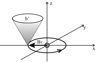
In the Time-Orbiting-Potential (TOP) trap [26] the losses of the quadru-pole trap are avoided by use of a rotating magnetic bias field BT OP added to the quadrupole field (see fig. 1.6). The B = 0 point moves, because of the rotating bias field, in a trajectory called the circle-of-death, because the atoms that cross it undergo a spin flip and then are lost from the trap. The radius of the circle of death is rcod ∝ (Btop/b0)1/2. The displacement speed of the B = 0 point must be such that the atoms cannot follow its trajectory; the potential felt by the atoms then corresponds to the instantaneous potential integrated in time:

U(x, y, z) = Z

(22)

Figure 1.6: The TOP trap. A rotating magnetic bias field causes a continuous displacement of the B = 0 point in order to avoid spin flip losses at the center.

It can be shown that the shape of the integrated potential is, close to its min-imum, parabolic, with its minimum Bmin 6= 0, and with average frequency:

ωho = (ωxωyωz)1/3 = b0 √ BT OP r µ m (1.35)

1.7 The dipolar trap

An alternative method for trapping cold atoms without using spontaneous emission processes is to exploit the dipolar force that emerges when the atoms are illuminated by a laser beam [27]. This force emerges due to the electric field carried by light:

E(r, t) = Eωe−iωt+ E−ωeiωt (1.36)

where E−ω = E∗ω. The resulting potential experienced by the atoms is:

U = −dEω (1.37)

where d is the atomic electric dipole. Because of the potential (1.37), the ground state of the atoms changes as:

∆Eg = X e hg|dEω|ei 1 Eg− Ee+ ~ω he|dE−ω|gi, (1.38)

where the sum is over all the excited states. In fact in Eq. (1.36), the classical field Eωe−iωtcorresponds to the absorption of a photon in a quantum

(23)

1.7 The dipolar trap 13

Figure 1.7: Dipolar confinement along the gravity (z) direction created by a laser beam with λ = 1030 nm, w0 = 46 µm and of power P = 1.1 W. Vdip is the resulting trap depth.

mechanical treatment, while the field E−ωeiωt corresponds to the emission of a photon.

After some calculations, Eq. (1.38) becomes: ∆Eg = −

1

2α(ω)hE

2_{(r, t)i}

t (1.39)

where E = Eˆ², h·it corresponds to a time average and α(ω) is the atomic polarizability: α(ω) =X e 2(Ee− Eg) |he|dˆ²|gi|2 (Ee− Eg)2− (~ω)2 . (1.40)

The change in energy of the ground state of the atoms can be seen as being due to the presence of an effective potential Vef f. Therefore, the atoms experience a force: F = −∇Vef f = − 1 2α(ω)∇hE 2_{(r, t)i} t. (1.41)

It is important to note from Eq. (1.40) that the dipolar force (1.41) is attractive if ~ω < Ee − Eg, i.e. the optical field is red detuned, while it is repulsive if ~ω > Ee − Eg, i.e. the optical field is blue detuned. In the description given above, the effect of spontaneous emission has been ignored. This approximation is valid in the limit that the detuning of the optical field is much larger than the frequency of the atomic transition:

|∆| = |~ω − (Ee− Eg)| À (Ee− Eg). (1.42) Therefore, within this approximation the light excites the atoms to virtual energy levels, and then the atoms decay to the ground state with a stimulated

(24)

emission process. The absence of spontaneous emission processes, i.e., photon scattering, makes the heating of the sample negligible.

Therefore, a red detuned optical laser creates a trap for the atoms. This trap is usually called dipolar trap. Its depth in Kelvin is:

Vdip = ~Γ2 π∆IsatkB P w2 0 (1.43) where P is the power of the laser beam and w0its waist. The radial frequency

of the dipolar trap is:

ωdip = s 2Γ2_~ π|∆|mIsat √ P w2 0 . (1.44)

1.8 The Experiment

The first step of our experiments is the production of Bose-Einstein con-densates of 87_{Rb atoms. This is an alkali element, i.e., of the group 1A}

in the Mendeleev periodic table, with the valence electron in the 52_S 1/2

or-bital. The lowest energy transitions are hence to the 52_P

1/2 and to the 52P3/2

levels, usually called the D1 and D2 lines, centered at 795 nm and 780 nm respectively. The optical transition we used to cool the atoms was the D2 line, whose spectrum is shown in figure (1.8), where the hyperfine levels of the 52_S

1/2 and 52P3/2 states are called F and F0 respectively. The ground

state hyperfine level used in our experiment was |F = 2i. Therefore, the frequency of the light used for the optical molasses and the MOT was near resonant to the transition |F = 2i → |F0 _{= 3i, the so-called laser cooling} transition, and hence only the atoms in the |F = 2i level were trapped in the MOT. However, this laser cooling transition is not closed: the atoms can be off-resonantly excited to the |F0 _{= 2i level, then decaying to |F = 1i. This} effect would cause a depletion of the number of atoms in the MOT. In order to circumvent this problem, a light near resonant to the |F = 2i → |F0 _{= 2i} transition was added to the laser cooling light, hence re-pumping the atoms in the |F = 1i level to the |F = 2i one. This light is called re-pumper.

1.8.1 Laser sources

The light for the laser cooling and the re-pumper was provided by two master lasers, whose output was then optically amplified in order to have the power needed for the experiment. A master laser was composed of a commercial laser diode, whose natural linewidth was of the order of few MHz. In order to reduce the linewidth, the diode output was sent to a grating creating an

(25)

1.8 The Experiment 15

Figure 1.8: Scheme of the D2 line of 87_Rb

external cavity with its first order of diffraction. At the back of the grating a piezo electric transducer was placed to vary the cavity length. The diode and the grating were placed in a home-made mount, stabilized in temperature with two Peltier elements with more than 0.01K of precision. Moreover, the current was supplied by external batteries rather than power supplies in order to avoid any coupling to the usual line noise.

The stability of the frequency of the master laser output is a crucial point in a cold atoms experiment. This goal was fulfilled by locking the laser frequency to an atomic transition. This was realized by sending a small portion of the laser output to an optical circuit. There, two beams were sent almost counterpropagating to a cell containing thermal vapor of Rb, one of them being stronger than the other. This beam (pump) saturated the transition, so it was possible to measure the saturated absorption spectrum by measuring the power of the weaker beam with a photodiode. Its output was used to create an error signal then sent to the piezoelectric transducer.

The output power of the two master lasers was ∼ 20 mW. The re-pumper light was then amplified by injecting a slave laser diode, whose output power

(26)

Figure 1.9: Scheme of the vacuum chamber. The magnetic field coils and both the 2D and 3D MOT laser beams are not shown.

was ∼ 55 mW. The master used for generating the laser cooling light was amplified in two stages: the master light injected a slave diode laser whose output was in turn used to inject a MOPA amplifier, whose output power was up to 600 mW. This light was used for all the purposes of the experiment, by splitting it and varying its frequency with acousto-optic modulators (AOMs).

1.8.2 The vacuum chamber

The apparatus was composed of two quartz vacuum cells placed at opposite sides of a central body. This was made of steel and internally devided by a septum (see Fig.(1.9)) that divided the vacuum chamber into two parts, connected only by a hole placed in the center of the internal septum, where a carbon tube was placed. The two cells had a square section and different sizes: (49 × 49 × 100) mm and (24 × 24 × 90) mm. Two ionic pumps were connected with the two parts of the vacuum chamber, in order to have a pressure ∼ 10−9_{mbar in the big cell and ∼ 10}−11_{mbar in the science cell} , where the experiments are performed (for this reason called the ”science cell”).

The Rb atoms were provided by two pairs of dispensers: electric resistances whose surface was covered with Rb, which was emitted when an electric current flowed in them. The dispensers were placed close to the big cell, where a two dimensional MOT was created by two pairs of counterpropagating laser

(27)

1.8 The Experiment 17 beams circularly polarized with waist w0 = 12 mm. These were detuned by

∆ = −2.4Γ from the |F = 2i → |F0 _{= 3i transition (Γ = 6.065 MHz is the} natural linewidth of the |F0 _{= 3i level), and a repumper beam was added to} them. The 2D MOT magnetic gradient was b0 _{= 11 G/cm.}

In the 2D MOT the atoms were collected in a cigar shaped cloud, whose long axis was parallel to the carbon tube. In the same direction, a near resonant laser beam (the ”pushing beam”) was sent in order to push the atoms from the 2D MOT cell to the science cell through the carbon tube. The corresponding atomic flux was collected by a 3D MOT in the science cell.

1.8.3 The 3D MOT

The 3D MOT was created by splitting a ∼ 30 mW beam into six beams of waist w0 = 8 mm. The beams were directed to the cell as three mutually

orthogonal counterpropagating pairs. A repumper light was added to two of these three pairs. The 3D MOT beams were detuned by ∆ = −2.5 Γ from the |F = 2i → |F0 _{= 3i transition. The magnetic gradient for the MOT was} b0 _{= 6.6 G/cm.}

The flux of atoms from the 2D MOT led to a continuous loading of the 3D MOT. This loading process was counteracted by an atoms loss process that was mainly due to collisions with background atoms. After ∼ 90 s of loading the MOT reached a stationary size, and up to 2 · 109 _{atoms were trapped.}

A portion of the light scattered by the atoms was collected by a lens and sent to a photodiode, whose signal was proportional to the number of atoms in the MOT. This reference was used in order to start the experiments with clouds of roughly the same size. Loading times of 25 − 40 s were usually sufficient in order to trap enough atoms before starting sub-Doppler and evaporative cooling.

1.8.4 The magnetic field

For trapping, cooling and displacing the atomic cloud several magnetic fields were used in the experiment.

• The quadrupole field. This was created by six cylindrical pancake-shaped coils placed along the direction of gravity z, that was hence the strong axis with the largest field gradient. In order to create a spatial magnetic gradient, the three coils above the science cell were in anti-Helmholtz configuration with respect to the three coils below the science cell (see Fig.(1.10)). The coils were made of copper and were covered with an insulating sock. The wires used for the coils

(28)

Figure 1.10: Schematic diagram of the mount of the coils for the magnetic gradient (shaded) and the rotating bias field (white). The science cell is at the center of the coils.

were hollow, and a continuous water flow inside them cooled the coils. The resulting magnetic gradient had cylindrical symmetry so that its modulus in the z direction (the strong axis) was 2b0_{, while in the x, y} directions it was b0_{. Magnetic gradients up to b}0 _{= 366 G/m were} created when the current was 226 A. This value was reached in 4 ms, while the time for switching off the field was of the order of 10 µs. • The rotating bias field. This field BT OP was created by two pairs of

coils: a pair of circular coils that were placed in between the quadru-pole coils, and a pair of square coils in the orthogonal direction (see Fig.(1.10)), both in Helmholtz configuration. The current flowing in each pair oscillated in time, and the pairs were mutually dephased by π/4: Icircular = IT OP sin(ωt), Isquared = IT OP sin(ωt + π/4), with ω = 10 KHz. The maximum value of the field was BT OP = 38 G. The cooling of the coils was assured by their contact with the water-cooled quadrupole coils.

• The compensation coils. These were three muthually orthogonal pairs of coils in the Helmholtz configuration. The current flowing in these coils was of the order of 100 mA. The magnetic field created by these coils was used to compensate the external fields, such as the earth’s magnetic field and the magnetic field created by the ion pumps. • The extra-compensation coil. This was a single coil placed above and

(29)

1.9 The experimental sequence 19 parallel to the quadrupole coils. Its role was to create a magnetic field that was varied during the experiment in order to be able to change the position of the cloud along the z-axis and hence to minimize the losses when the trap was changed, e.g., when passing from the TOP to the dipolar trap.

1.9 The experimental sequence

After that ∼ 109 _{atoms were trapped in the MOT, sub-Doppler and}

evap-orative cooling were used in order to create a Bose Einstein condensate, which was the starting point for all the experimental investigations reported in this thesis. The different stages for driving the atoms through the BEC phase transition constituted a temporal sequence during which several exper-imental parameters (laser frequency and intensity, magnetic fields etc.) were changed. Every single experiment performed was destructive, so the whole process had to be restarted from the 3D MOT loading.

The experimental sequence was controlled by a computer, which controlled in time (within a resolution of 10 µs) all the experimental parameters. In the following, the experimental sequence for the creation of a Bose-Einstein condensate is listed in chronological order.

• The compressed MOT (C-MOT). During this phase the size of the MOT was reduced by decreasing the magnetic gradient (to b = 2.6 G/cm) and increasing the detuning (to ∆ = −4.8 Γ) of the laser. This phase was 200 ms long. This compression was done in order to optimize the loading into the TOP trap.

• The Molasses. During this phase, which was 6 ms long, the magnetic gradient was switched off and the detuning of the laser increased to ∆ = −5.0 Γ. The sample was cooled to the sub-Doppler regime, reaching at the end of the stage a temperature around 15 µK. Moreover, during the molasses phase the capacitors of the quadrupole field power supply were charged, in order to reduce the rising time of the magnetic gradient in the TOP trap.

• Optical pumping. This phase consisted of three light pulses that pumped the atoms into the |F = 2, mF = 2i state. The light frequency was res-onant with the |F = 2i → |F0 _{= 2i transition, and the quantization} axis was defined by the rotating bias field BT OP that was switched on with amplitude BT OP = 3.8 G. In order to pump the atoms into the |F = 2, mF = 2i state, the selection rule for the light-induced atomic transition had to be ∆mF = +1. This condition was realized when the

(30)

light was circularly polarized σ(+) _{and the magnetic field was pointing}

in the same direction as the light wavevector. Because the direction of BT OP rotated with frequency 10 KHz, the optical pumping was re-alized by sending to the atoms three light pulses of 10 µs duration and synchronized with the BT OP field in order to illuminate the atoms only when BT OP was pointing in the desired direction.

• The TOP trap. At the end of the optical pumping stage the atoms were loaded into the TOP trap. This was done by increasing the magnetic gradient in 1 ms to b0 _{= 73 G/cm, while the rotating bias field was} turned on at its maximum value, in order to maximize the circle of death. After the loading, the trap frequencies were first increased in order to enhance the collision rate, and hence to create the conditions for an efficient evaporative cooling. The evaporative cooling was then realized by reducing the circle of death. At the end of the process the cloud contained ∼ 6 · 105 _{atoms at a temperature T = 2.5 µK.}

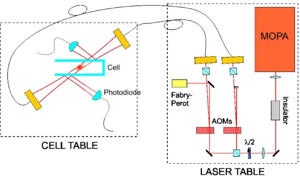
• The Dipolar trap. After the evaporative cooling in the TOP trap, the atoms were loaded into the dipolar trap. This was created by use of a Yb:YAG laser, with a maximum power of 5W and emitting at λ = 1030nm, i.e., far off-resonance from the Rb transitions. Its output was split into two beams, and each of them was sent to an acousto-optic modulator, and then to the atoms. There the two beams intersected at an angle ∼ 90◦_{, creating hence an optical trap for the} atoms. After passing through the science cell, each beam was collected and sent to a photodiode, whose signal was sent to a PID circuit. In this circuit the photodiode signal was compared to a reference from the computer, and the PID output was then used to control the power of the radiofrequency input of the corresponding AOM and hence the power of the dipolar beam. By these feedback circuits the power of each beam was controlled by the computer, and the noise in the beam powers was reduced to a signal-to-noise ratio S/N ∼ 10−4_{. The dipolar} beams had a maximum power of 1.2W each, and were focalized to the atoms with a waist w0 ∼= 46 µm. The corresponding maximum depth

of the optical trap was 7 µK, while the maximum mean frequency was ¯

ω = 490 Hz.

1.9.1 Bose-Einstein condensation

Once the atoms were loaded into the dipolar trap, evaporative cooling started in this trap as well. This was performed by ramping down in time the power of both the dipolar beams, so both the depth and the frequencies of the opti-cal trap were reduced. The overall ramp was formed by four linear ramps of

(31)

1.9 The experimental sequence 21 decreasing gradient. This cooling stage was 2.5 s long, and at its end a Bose Einstein condensate of up to 105 _{atoms was created. Fig.(1.11a)) reports}

the CCD image of a sample formed by a thermal part over which a conden-sate fraction emerges. The density profile reported in Fig. (1.11 a)) shows the typical bimodal distribution (see Fig.(1.1)) in which the Bose Einstein condensate emerges as a density peak surrounded by a broader distribution of thermal atoms. Fig. (1.11 b)) shows the CCD image of an almost pure condensate.

Figure 1.11: Absorption images of the cloud at the end of the evaporative cooling in the dipolar trap. The lines correspond to the density profiles. a) Image of a cloud in which ∼ 30% of the atoms are condensed. The line over the density profile is a fit with a sum of two gaussian functions. b) Image of a cloud which is an almost pure BEC.

Imaging the cloud

At the end of the evaporative cooling the atoms were released from the trap and allowed to expand in free space, in order to decrease the density of the cloud. After a certain time (called time of flight) of the order of ∼ 10−20 ms a resonant light pulse of 10 µs duration was sent to the atoms and then collected by a CCD camera, in which the shadow of the atomic cloud was imaged. This signal was proportional to the column density of the condensate. The CCD camera was purchased from DTA, featuring a Kodak Chip (KAF 1400) with pixel size 6.8 × 6.8 µm, whose quantum efficiency was 40% at 780 nm. In front of the CCD camera an objective (Rodenstock Aporadagon) of focal length f = 75 mm and f-number f /# = 4.5 was placed. The objective was optimized for 1:2 reduction, but it was used reversed in order to have a magnification of ∼ 2. The system was focused by minimizing the apparent size of small atomic clouds imaged on the CCD. The calibration of the image

(32)

size was done by performing an experiment of free fall of the condensate under gravity.

(33)

23

Chapter 2 Optical lattice

The experiments described in this thesis were performed on Bose Einstein condensates in a periodic potential. This was created optically by the inter-ference of two laser beams, far detuned from the atomic transitions. This chapter gives both the theoretical and the experimental background of the physical system that forms the basis of our experiments.

2.1 Introduction

At the end of the 1970s, the technological developments in experimental laser physics allowed to realize experiments on the interactions between atomic beams and standing waves created by the interference of laser beams [28]. The study of the interactions between atoms and light of frequency near resonant to some atomic transition eventually led to the realization of laser cooling [4, 5, 6].

On the other hand, the study of the interactions of atoms and far off-resonant light also paved the way towards ”atom optics” [9, 29]. Within this subject, many predicted effects were observed using atomic beams as a sample [10, 30]. This interest was renewed once cold atomic clouds were realized, and the periodic potentials created by light interference (usually called optical lattices) were used to observe basic phenomena of solid state physics [31, 32, 33].

More recently, Bose-Einstein condensates were loaded into optical lattices [11]. The coherence of the BECs permitted to study more accurately solid state physics effects [12], as well as the physics of strongly interacting systems [34]. Within this research field, the emergence of phase transitions such as the superfluid-Mott insulator [35] led to the use of optical lattices for studying the physics of phase transitions.

(34)

2.2 Atom optics

A standing wave is created by the interference of two laser beams at frequency ωL= 2πc/λ. If the two beams propagate along the x axis and have the same polarization ˆ², the resulting total electric field carried by the light is

E(r, t) = E0sin(kLr + ωLt)ˆ² + E0sin(kLr − ωLt)ˆ², (2.1)

where E0 is the amplitude of each field, and kL= 2π/λ the light wavevector. Under the hypothesis that the frequency of the laser beams is far off-resonant from the closest atomic transition at frequency ω, i.e. |∆| = |ωL− ω| À ω, then spontaneous emission can be neglected. Therefore, the stimulated emis-sion process in which j photons are transferred from one laser beam to the second one causes a change of the atomic momentum of ∆p = 2j~kL [36]. In this atom optics approach the atomic states are plane waves that experience Bragg diffraction from the standing wave. In a j-th order diffraction process, energy conservation reads:

~2_p2 2m = ~2_{(p + ∆p)}2 2m = ~2_{(p + 2j~k} L)2 2m . (2.2)

The condition (2.2) leads to the atom optics analogue of the Bragg law:

p = −j~kL. (2.3)

Let us consider a first-order diffraction process in which the initial atomic momentum is ~kL. The state of the system after a time t is:

Ψ(x, t) = c(−1, t)| − 1, gi + c(0, t)|0, ei + c(1, t)|1, gi (2.4) where |n, g(e)i is the free particle state of the ground (excited) level with momentum n~kL. Under the dipole approximation, the Hamiltonian of the system is [29]:   ~ω0 −ie −iωLt~Ω r/2 ie−iωLt~Ωr/2 ieiωLt~Ωr/2 −~ωrec 0 −ieiωLt~Ω r/2 0 ~ωrec   , (2.5) where:

Ωr= ℘E0/~ single beam Rabi frequency

℘ electric dipole moment

ωrec = Erec/~ recoil frequency Erec = ~2k2L/2m recoil energy

If at t = 0 the atomic momentum is ~kL, so that the initial state is:

(35)

2.2 Atom optics 25

Figure 2.1: First order Bragg transition. The atom initially in the state |1, gi absorbs a photon, thus reaching the virtual level represented by the dotted line. A subsequent stimulated emission of one photon into the other beam forming the standing-wave field takes the particle to the level |−1, gi. then the state of the system at time t is:

c(−1, t) = ie−iΩ(2)r /2_sin Ã Ω(2)r t 2 ! c(0, t) = 0 c(1, t) = e−iΩ(2)r /2_cos Ã Ω(2)r t 2 ! , (2.7)

(36)

where the two photon Rabi frequency Ω(2)r is given by: Ω(2) r = Ω2 r 2∆. (2.8)

The atomic momentum oscillates in time from ~kL to −~kL, and the proba-bility of finding the atoms in the initial state is thus:

P (p = ~kL, t) = sin Ã Ω(2)r 2 t ! (2.9) This process is known as Pendell¨osung oscillation [37] and it is the analogue of the Rabi oscillations in a two-level system.

2.3 Solid state approach

The effects of a standing wave on an atomic sample can be studied by use of the dressed-atom approach [21], for which the light interaction results in a change of the atomic adiabatic levels. Let us consider a system with one ground state |gi and one excited state |ei. The Hamiltonian reads:

H = µ −~∆ ~Ωrsin(kLx) ~Ωrsin(kLx) 0 ¶ , (2.10)

where x is the mean value of the position and can therefore be considered as a parameter. If one solves the problem by adiabatically eliminating the excited state |ei, the energy of the ground state is:

Eg = ~ Ω2 r ∆ sin 2_(k Lx). (2.11)

The eigenvalue (2.11) can be considered as a conservative potential expe-rienced by the atoms in the ground state. In the case of far off-resonant light, the population of the excited level is infinitesimally small, therefore the Hamiltonian of the system is:

H(x) = p2 2m + V0 2 cos(2kLx), (2.12) where V0 = ~ Ω2 r ∆ = 2~Ω (2) r (2.13)

is the lattice depth, usually expressed in units of recoil energies Erec = ~2_k2

(37)

2.3 Solid state approach 27

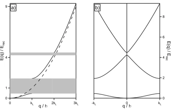
Figure 2.2: a) the dispersion law for the free particle (dashed line) is plotted together with the energy-vs-momentum curve in the presence of the periodic potential (continuous line): the shaded regions correspond to energy gaps; b) the energy spectrum is folded into the first Brillouin zone

Before solving the eigenvalue problem of the Hamiltonian (2.12), let us reanalyze the first order Bragg scattering process within this picture. As stated in the previous section, if the atomic momentum is ~kL the evolution of the atomic wavefunction involves only the states with momentum ±~kL. In the base formed by the plane waves |kLi, | − kLi, the Hamiltonian (2.12) reads: H = µ Erec V0/4 V0/4 Erec ¶ . (2.14)

|kLi = 1 √

(38)

The atomic wavefunction at time t is therefore: |ψ(t)i = √1 2e iErect/~_(e−iV0t/4~_|ψ 1,kLi + e iV0t/4~_|ψ 2,kLi). (2.17)

The probability at time t that the atomic momentum has at the initial value ~kL is: |h+kL|ψ(t)i|2 = sin2 µ V0 4~t ¶ , (2.18)

that is equal to the probability (2.9) that was found in the atom optics picture.

Apart from demonstrating that the Hamiltonian (2.12) describes this phys-ical system as the atom optics picture does, the previous calculations allow us to observe one of the key features of the energy spectrum of this problem. The Hamiltonian (2.14) has two eigenvalues E1(kL) and E2(kL) that are not degenerate, but have a difference in energy ∆E1 = E2(kL) − E1(kL) = V0/2.

This corresponds to an energy gap in the dispersion law, because a region of forbidden energies emerges. Energy gaps of different sizes emerge in the dis-persion law periodically with period ~kL (see Fig.(2.2)). The dispersion law is therefore divided into branches, called energy bands, that can be labeled by an index n: in first order Bragg scattering the two eigenvalues (2.15) cor-respond to the first (n = 1) and the second (n = 2) band. The energy bands can be folded into the region [−~kL, ~kL] of momentum space, called first Brillouin zone, and the momentum p is substituted by the quasimomentum q = p + ~K, where K = jkL, j integer, is a generic reciprocal lattice vector.

The band structured dispersion law of an atom in an optical lattice recalls the dispersion law of an electron in a crystal. In fact, as in this physical system, the Hamiltonian (2.12) is periodic in space: H(x) = H(x + dL), where dL = λ/2 is the lattice constant. Therefore the Bloch theorem holds [38], and the eigenstates of the Hamiltonian (2.12) are of the form:

|ψn,q(x)i = X

q

eiqx_|u

n,q(x)i (2.19)

where the functions |un,q(x)i are periodic in space: |un,q(x)i = |un,q(x + dL)i. In the case of a sinusoidal potential as in Hamiltonian (2.12), the wavefunctions (2.19) are the Mathieu functions [39]. It is interesting to point out the link between the atom optics and the solid state approach. This can be done by expanding the periodic functions |un,q(x)i in the Fourier series:

|un,q(x)i = X

j

(39)

2.4 The tight-binding approximation 29 The exponential terms in (2.20) correspond to plane waves of momentum 2j~kL:

|un,q(x)i = X

j

cn,q|2jkLi. (2.21)

Therefore the eigenfunctions (2.19) can be written as a sum of plane waves: |ψn,qi =X

j

cn,j(q)|q/~ + 2jkLi. (2.22)

The analogies between the problem of an atom in an optical lattice and an electron in a crystal suggest that solid state physics can be explored in a different framework. In fact, with respect to solid state experiments, there are several advantages in studying solid state physics using a condensate in an optical lattice. First, the optical lattice can be easily manipulated: its depth and lattice constant can be varied, it can be switched on and off in a short time, and different lattice structures can be implemented [40]. Moreover, an optical lattice has no impurities, resulting in an increase of the mean free path. Finally, the dynamics of the atoms can be observed both in real and momentum space, and the role of nonlinearity in the system can be explored.

2.4 The tight-binding approximation

In the previous section the Mathieu functions |ψn,q(x)i were expanded in the basis of the plane waves |q/~+2jkLi. Another full basis of the system is given by the Wannier functions. The Wannier function |φn(x − xl)i is centered at the l-th lattice site of coordinate xl, and it is defined as the Fourier transform of the Mathieu function [38]:

φn(x − xl) = 1 2~kL Z _~k_L −~kL dqe−ildLq_ψ n,q(x). (2.23)

The Wannier functions are localized, and Wannier functions centered at dif-ferent lattice sites are orthogonal:

hφn(x − xl)|φn(x − xj)i = δl,j. (2.24) Because the Wannier functions form a complete set, the Mathieu functions can be expanded in this basis:

|ψn,q(x)i = X l cl|φn(x − xl)i = 1 √ N X l eildLq_|φ n(x − xl)i. (2.25) The Hamiltonian (2.12) can be expressed in the Wannier basis as well. The Hamiltonian matrix elements are:

(40)

where for simplicity we restricted the analysis to the fundamental band, i.e., n = 1. In the case of a deep lattice one can neglect all the interactions between lattice sites that are not nearest neighbors:

Hl,j = 0 for j 6= l, l ± 1. (2.27)

This is a tight binding approximation that makes the Hamiltonian matrix tri-diagonal. The terms of the principal diagonal of the matrix are:

Hl,l = hφ1(x − xl)|H|φ1(x − xl)i = E0, (2.28)

while the off-diagonal terms are:

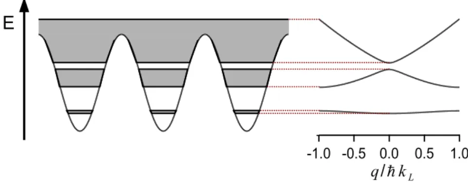
Hl,l±1= hφ1(x − xl)|H|φ1(x − xl±1)i = γ. (2.29) The off-diagonal terms connect neighboring lattice sites. The physical process that is behind these connections is the inter-well tunneling. This point will be cleared when the Bose-Hubbard model will be introduced. The dispersion law for the fundamental band can be calculated by use of the expansion of the Mathieu function for n = 1 in the Wannier basis (2.25) [38]:

E1(q) = hψ1,q(x)|H|ψ1,q(x)i = E0+ 2γ cos(qd/~). (2.30)

2.4.1 The Bose-Hubbard model

In 1998 Jaksch et al. [41] proposed to use a tight-binding-like approximation to write an Hamiltonian for a condensate of N interacting bosons loaded in a deep lattice. The starting point is the many-body Hamiltonian for the Bose-field operators: H = Z d3r ˆΨ†(r) µ − ~ 2 2m∇ 2₊ V0 2 cos(2kLx) ¶ ˆ Ψ(r)+ +1 2 4πas~2 m Z d3_{r ˆ}_Ψ†_{(r) ˆ}_Ψ†_{(r) ˆ}_{Ψ(r) ˆ}_Ψ(r), (2.31)

where ˆΨ(r) is the Bose field operator in a three dimensional space of coor-dinate r = (x, y, z), and the 1D optical lattice is along the x direction. The 3D Hamiltonian (2.31) is separable in three 1D Hamiltonians. In the y, z directions the Bose-field operator can be approximated by a single particle wavefunction Φ(y, z) as shown when the Gross-Pitaevskii equation was de-rived. In the x direction, the Bose field operator can be expanded in terms of the boson creation and annihilation operators a†_l, al at the single lattice site:

ˆ

Ψ(†)_{(x) =}X

l

(41)

2.4 The tight-binding approximation 31 where the amplitude of each term is given by the corresponding Wannier function. The expansion (2.32) can be now substituted into the Hamiltonian (2.31). If, as in the tight binding approximation, only the interactions be-tween next neighboring sites are considered, then the Hamiltonian along the x axis is: H = −JX hl,ji a†_laj + U 2 X l nl(nl− 1) (2.33) where:

• the sum hl, ji is over nearest neighbor sites

• nl = a†lal is the number operator that counts the number of atoms in the n-th site • J = R dxφ(x − xl) ³ −~2 2m∇2+ V0 2 cos(2kLx) ´ φ(x − xj) is the hopping matrix element that considers the tunneling from one lattice site to a neighboring one. J is equal to the off diagonal term γ (2.29) of the Hamiltonian that was found in the tight binding approximation. • U = 1

24πas~

2

m R

dx |φ(x)|4 is the interaction energy of two atoms occupy-ing the same lattice site.

The Bose-Hubbard Hamiltonian (2.33) expresses therefore that the dynamics of cold atoms in a deep lattice depend only on two parameters: the on-site interaction U and the tunneling between lattice sites J. Their dependence on the lattice depth V0 is [42]:

J = √4 πErec µ V0 Erec ¶ exp Ã −2 r V0 Erec ! U = √8 πkasErec µ V0 Erec ¶_1/4 (2.34)

The preceding formulas demonstrate how the evolution of an atomic sample in an optical lattice can be controlled by just varying the lattice depth. Experimentally, this can be done very easily by changing the power of the laser beams creating the lattice. However, by changing the lattice depth both U and J are varied at the same time. The interaction U can be controlled independently by using a Feshbach resonance [43, 44], that allows to vary the scattering length as. On the other hand, one can control independently the tunneling parameter J by strongly driving the lattice. This technique has been explored in an experiment described in Chapter 5.

(42)

2.5 The lattice and a force

The flow of an electric current in a conductor is one of the fundamental problems of solid state physics. Theoretically, this results in the problem of a crystal Hamiltonian to which an external force is added. This same physical system can be implemented in an experiment of cold atoms in an optical lattice by applying a force F to the atoms.

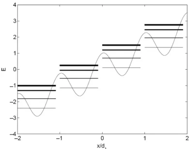
One of the first solid state phenomena that was observed in an atomic physics experiment were the Bloch oscillations [32]. In order to observe how this effect emerges, let us start from the problem of an atom loaded into an optical lattice and on which a force is exerted. The force leads to a linear potential that must be added to the optical lattice Hamiltonian (2.12):

H = Hlattice+ HF = p2

2m +

V0

2 cos (2kLx) − F x. (2.35) Let us assume that one atom is loaded in the fundamental band of an optical lattice with initial quasimomentum q = 0, and to exert at t = 0 a constant force F on the atom. At time t the atomic wavefunction is:

|ψ(x)it = exp µ −i ~(Hlattice+ HF)t ¶ |ψq=0(x)it=0. (2.36) The exponential operator into Eq.(2.36) can be transformed in a product of exponential operators by use of the Baker-Campbell-Hausdorff formula [45]. In this operator product, all the terms containing the momentum operator p give no contribution. Therefore, Eq.(2.36) reduces to:

|ψ(x)it= exp µ −i ~Hlatticet ¶ exp µ −i ~HFt ¶ |ψq=0(x)it=0 = exp µ −i ~Hlatticet ¶ exp µ i ~F xt ¶ |ψq=0(x)it=0 = exp µ −i ~Hlatticet ¶ |ψq(t)(x)i. (2.37)

The state of the atom remains an eigenstate of the Hamiltonian Hlattice but with quasimomentum changing in time according to

q(t) = F t. (2.38)

In the more general case of a time dependent force F (t) Eq.(2.38) becomes: q(t) =

Z

F (t)dt. (2.39)

Eq.(2.37) states that the evolution of the wavefunction of the atom cor-responds to an evolution of its quasimomentum in momentum space. Let us follow this evolution in the case of a constant force step by step: