In vitro assessment of the primary stability of the acetabular component in hip arthroplasty

(1)

___________________________________________________________________________________ ALMA MATER STUDIORUM - UNIVERSITÀ DI BOLOGNA

CAMPUS DI CESENA

SCUOLA DI INGEGNERIA E ARCHITETTURA

CORSO DI LAUREA MAGISTRALE IN INGEGNERIA BIOMEDICA

TITOLO DELLA TESI

IN VITRO ASSESSMENT OF THE PRIMARY STABILITY

OF THE ACETABULAR COMPONENT IN HIP

ARTHROPLASTY

(Valutazione sperimentale della stabilità primaria della componente acetabolare nell’artroplastica dell’anca)

Tesi in MECCANICA DEI TESSUTI BIOLOGICI

Relatore Presentata da

Chiar.mo Prof. Luca Cristofolini

Mariateresa Linsalata

Co-Relatore

Ing. Federico Morosato

Sessione III

(2)

(3)

3

ABSTRACT

In Europe, more than 700,000 hip arthroplasties are performed annually. The failure rate of hip implants is 2-8% (at 10 years). Of this, more than 50% is due to the aseptic mobilization of the acetabular component (more than to the femoral component).Some follow-up clinical studies demonstrate a correspondence between the loss of the primary stability and the late aseptic loosening of the prosthesis, hence, the need to investigate more thoroughly the primary stability of the acetabular component. Despite the presence in literature of in vivo evaluations carried out through radiographic criteria, there are no exhaustive pre-clinical studies conducted in vitro with respect to primary stability.

The central aim of this project is to create a pilot-test for the in vitro evaluation of the primary stability of a commercial acetabular component, implanted in a synthetic hemipelvis (implanted by press-fit surgical procedure). The micromovement evaluation includes a multi-faceted approach, consisting in using the Digital Image Correlation (DIC) and linear displacement sensors. To adapt and improve the performance of the two measuring instruments, the study aims to: (1.a) optimize the measurements obtained from image correlation, (1.b) create and perform the internal calibration procedure of the displacement sensors and optimize the measurements obtained from the sensors themselves (used as spot-check of the entire pilot-test). The second part of the work is to implement a reliable methodology for calculating the relative roto-translations between cup and bone, applying a physiological critical load on the specimen. The creation of a dedicated algorithm provides, therefore, to evaluate: (2.a) permanent migration and (2.b) inducible micromotion. The use of image correlation was a focal point for the study. Thanks to the power of the DIC in analysing displacement motion and strain in full-field, in contact-less and relying on stereophotogrammetry, for the first time it was possible to obtain 3D information of the migration vector of the cup. Furthermore, by creating an optimized procedure for the calibration of the DIC, it was possible to report all the measurements obtained from the pilot-test, to the Anterior Pelvic Plane (reference frame with clinical relevance).

The results obtained from the pilot-test highlight the reliability of the procedure, proposing it as

(8)

(9)

9

RIASSUNTO

In Europa, più di 700'000 interventi di artroplastica d’anca vengono effettuati annualmente. Il tasso di fallimento della chirurgia è del 2-8 % (a 10 anni). Di questo, più del 50% è dovuto alla mobilizzazione asettica della componente acetabolare (più che ad un fallimento legato alla componente femorale). Alcuni studi clinici di follow-up, dimostrano esserci una corrispondenza tra la perdita della stabilità primaria e la mobilizzazione asettica tardiva della protesi. Da ciò nasce l’esigenza di investigare più a fondo sulla stabilità primaria della componente acetabolare. Nonostante la presenza in letteratura di valutazioni condotte in vivo, specialmente attraverso criteri radiografici, mancano studi esaustivi di carattere pre-clinico condotti in vitro rispetto alla stabilità primaria.

Lo scopo centrale di questo progetto di tesi è quello di creare un pilot-test per la valutazione in

vitro della stabilità primaria di una componente acetabolare commerciale, impiantata in una

emipelvi sintetica (senza cemento, attraverso la procedura chirurgica press-fit). La valutazione dei micromovimenti prevede un approccio multiplo, costituito dall’utilizzo della Digital Image Correlation (DIC) e di sensori lineari di spostamento. Per adeguare e migliorare le prestazioni dei due strumenti di misura, lo studio prevede: (1.a) l’ottimizzazione delle misure ottenute dalla correlazione di immagini, (1.b) creare ed effettuare la procedura di calibrazione interna dei sensori di spostamento e l’ottimizzazione delle misure ottenute dai sensori stessi come monitor dell’intero pilot-test. La seconda parte del lavoro si prone di implementare una metodologia affidabile per il calcolo delle roto-traslazioni relative tra coppa e osso. La creazione di un algoritmo dedicato, prevede, quindi, di valutare: (2.a) la migrazione permanente e (2.b) i micromovimenti inducibili dai picchi di carico.

L’utilizzo della correlazione di immagini è risultato un gran punto di forza dello studio. Grazie al potere della DIC nell’elaborare spostamenti e deformazioni a tutto campo, senza contatto e in stereofotogrammetria, per la prima volta è stato possibile ottenere informazioni 3D del vettore migrazione della coppa. Inoltre, creando una procedura ottimizzata dell’allineamento del provino sotto la macchina, si sono potute riferire tutte le misure ottenute dal pilot-test, all’Aneterior Pelvic Plane (sistema di riferimento di rilevanza clinica).

I risultati ottenuti dall’esecuzione del pilot-test mettono in luce l’efficacia della procedura creata, proponendola come modus-operandi per una campagna di test su emipelvi in composito e biologici.

(10)

(11)

11

1. INTRODUCTION

The aim of the introduction is to provide some information about the anatomy and the biomechanics of the pelvis, about the total hip arthroplasty and its failure risks. In addition, for a proper knowledge of the work, the primary stability definition is given, with a synthetize state of the art about its assessment. Finally, an overview about the sensors used for this study is presented.

1.1 ANATOMY OF THE PELVIS

1.1.1 Bone tissue

Bone tissue is a specialized form of the connective tissue. It is characterized by a mineralized extracellular matrix which lend stiffness and mechanical strength1_.

The bone is the major structural and supportive tissue of the body, constituting the skeleton2. The bone exerts important functions in the body, such as locomotion, support and protection of soft tissues, calcium and phosphate storage, and hosting of bone marrow3, 4

It is composed by the 25% of water, the 32% of organic matrix and the 43% of apatite mineral1. Bone exhibits four types of cells: osteoblasts, bone lining cells, osteocytes, and osteoclasts. Osteoblasts and osteocytes are involved in the formation and mineralization of bone; osteoclasts are involved in the resorption of bone tissue: despite its inert appearance, bone is a highly dynamic tissue that is continuously resorbed by osteoclasts and reconstituted by osteoblasts. There are evidences that osteocytes act as mechanosensors and orchestrators of this bone remodelling process5_{, necessary for fracture healing, skeleton adaptation to mechanical use} and for calcium homeostasis. Finally, flat-shaped osteoblasts become the lining cells that form a protective layer on the bone surface. Precisely, the lining cells are set in the inner surface of bones, which separates the bone from the marrow, called endosteum. The external surface of bones is composed by a high-vascularized soft tissue called periosteum6.

Bone tissue is a mineralized tissue of two types: cortical bone and trabecular bone.

The cortical bone represents the outer shell of bones and is composed by several closely packed osteons or harvesian systems. The osteon is a 150-250 micrometers cylinder in diameter, consisting of a central canal (harvesian canal) through which blood and lymphatics vessels and nerve run, surrounded by 4-20 concentric layers of lamellae7.

The trabecular bone consists in a network of about 0.2 mm-thick trabeculae, composed by packages of parallel lamellae, up to 1 mm long and 50-60 microns in section and linked by cemented lines. Here, the nutrients are directly taken from the mellow in the interstitial space between trabeculae. Trabecular bone density and orientation may widely vary within different anatomical sites depending on the mechanical role which locally cover; trabecular structure, in fact, results to be mainly oriented along the primary load direction8. Because of its structure, trabecular bone does not significantly contribute to the bone stiffness alone; however, due to the

(12)

cheaper metabolic cost (rather than the cortical) and in combination with the cortical bone, it covers an important role in terms of:

• stiffen the structure connecting the outer shell of cortical bone;

• support the layer of the cortex and distribute the loads in the case of lateral impacts; • support the articular cartilage and act as shock-absorber during load

• transfer and distribute the load to the surrounding cortical bone; • protect the cave bones from phenomena of instability (buckling)1_. Due to their shape, bones can be classified in:

• Long: characterized by a shaft, the diaphysis, that is much longer than its width, and by an epiphysis, a rounded head at each end of the shaft. They are made mostly of compact bone, with lesser amounts of marrow, located within the medullary cavity, and areas of spongy, cancellous bone at the ends of the bones;

• Short: they mostly withstand compressive loads and transfer loads between articular surfaces;

• Flat: these kind of bones (i.e. the pelvis) are made by a typical sandwich structure, with the thin layers of cortical bone carrying most of the load9. The thin layers are separated by the trabecular bone (Fig.1).

This structure is optimized for being characterized both by stiffness (high inertia) and tenacity, thus with high deformability and strength1.

Fig.1: Detail of the iliac crest flat bone.

(13)

13

1.1. 2 Optimized hip structure is functional to the load distribution

The concept that bone adapts to stress, or a lack of it, is known as Wolff’s law. It’s the reason why astronauts return with reduced bone density after floating in microgravity!10

The adaptive nature of bone lies in its ability to respond to the environment by conforming and reshaping itself constantly to accommodate life-time stresses experienced throughout daily activities11. Wolff’s law states that bone has the ability to adapt to mechanical loads: it means that the external and internal structure of bone changes depending on the load occurring in the bone. Especially with regard to implant technology and arthroplasty, bone adaptation (bone remodelling) plays an important role: if the biomechanical distribution of forces in and around the treated joint is reconstructed inappropriately during surgery, or if the design of the implant is improper, many complications can occur20.

This ongoing turnover of bone is a process of resorption followed by replacement of bone, with little changes in shape accomplished through osteoblasts and osteoclasts. Cells are stimulated by a variety of signals, maybe as the result of bone's piezoelectric properties, which cause bone to generate small electrical potentials under stress12_{. Approximately 10% of the skeletal mass of an} adult is remodelled each year13.

1.1.3 The pelvic girdle

The pelvic girdle is composed by two symmetrical flat bones that constitute the pelvic girdle, the bony structure that links the axial skeleton to the lower limbs. The hip bone presents three articulations:

• Sacroiliac joint: articulation with the sacrum (Fig.2.A).

• Pubic symphysis: articulation with the contro-lateral hip bone (Fig.2.B). • Hip joint: articulation with the head of the femur (Fig.2.C)14.

(14)

Fig.2: A. Sacroiliac joint in green; B. Pubic Symphysis articulation in green; C. Hip joint in green.

The hip bone is formed by three parts: the ilium, the ischium, and the pubis, fused together in the acetabulum, the socket in which the femoral head is inserted (Fig.3.A). The complete fusion of

ilium, ischium and pubis occurs at the end of the teenage years (14–16), with the calcification of

the triradiate cartilage (Fig.3.B).

A B

Fig.3: A. Anterior view of the pelvic girdle;

B.The hip bone of a 5 years old, with triradiate cartilage still present.

The acetabulum is supported by the anterior and the posterior columns (Fig.4.A). Because of their architecture, these columns act as struts, adding stability and transferring the forces exerted by the femoral head15_{. The two columns join superiorly to the acetabulum, forming a radiolucent triangle,} which gives flexibility to the acetabulum. The acetabular rim is inferiorly interrupted with the acetabular notch. Here the legamentum teres is originated and it directly links the acetabulum with the femoral head, allowing more stability to the joint. The legamentum teres is a somewhat flattened band inserted by its apex into the antero-superior part of the fovea capitis femoris. Under the notch there is the oval foramen, through which nutrient vessels and nerves reach the joint (Fig.4.B)16.

(15)

15

A B

Fig.4: A. Acetabular columns, acetabular notch and the radiolucent triangle labelled on figure; B. Legamentum teres;

The legamentum teres is the intracapsular ligament of the hip joint. The extracapsular ligaments are:

• the ileofemoral ligament (Fig.5.A), • the ischiofemoral ligament (Fig.5.B), • the pubofemoral ligament (Fig.5.A),

All three strengthen the capsule and prevent an excessive range of movement and dislocation in the joint 17.

A B

Fig.5: A. Pubofemoral ligament and ileofemoral ligament in anterior view; B. Ischiofemoral ligament in posterior view

(16)

1.1.3.4 The hip joint

A joint, or articulation, is a connection between two bones, which allows their relative movement. The hip joint, or acetabulo-femoral joint (art. coxae), is one of the largest among the synovial joints of the body, which are characterized by bones joined each other with a fibrous joint capsule that is continuous with the periosteum of the joined bones. The joint capsule is made up of an outer layer, the articular capsule, which keeps the bones together structurally, and an inner layer, the synovial membrane, which seals in the synovial fluid. The hip joint is formed by the femur and the acetabulum and its primary function is to support the weight of the body in both static and dynamic tasks ensuring relative movement between thighs and pelvis. It is a ball-and-socket joint, where the ball is the femoral head and the ball-and-socket is the acetabulum.

As a ball-and-socket joint, the allowable movements at the hip joint are three components of rotation:

• flexion and extension (in the sagittal plane of the body); • abduction and adduction (in the frontal plane of the body);

• intra and extra rotation (in the transverse plane of the body)10,18 _(Fig.6).

Fig.6: ball- and -socket simplified representation with allowed movements labelled.

These movements are limited both by the morphology of the hip bone and by the soft tissues, ligaments and muscular structures. In addition, the presence of osteophytes (referred to bone irregularities that form in joints margin to give more contact surface between articular bodies), along the acetabular rim (i.e. labrum), may constrain the joint mobility.

1.2 BIOMECHANICS OF THE HIP

Biomechanics is the science that studies the forces acting in the living body. Under gravity and other loads, controlled by the nervous system, human movement is achieved through a complex and highly coordinated mechanical interaction between bones, muscles, ligaments and joints within the musculoskeletal system. If any of these individual elements is injured or lesioned, the mechanical interaction will change, causing degradation, instability or disability of movement19_.

(17)

17

Thus, it’s necessary to study and to understand the body biomechanics to prevent injury, correct abnormality, and improve healing and rehabilitation.

Tab.1 shows the movements at the hip joint (with their own range of motion) and the muscles involved (Fig.7).

Tab.1: List of the kind of rotation (first column), the range of motion of the related rotation in human pelvis (degrees (°)) and the main muscles involved in the related rotation.20

Rotation Range of Motion Muscles involved

external rotation 30° with the hip extended 50° with the hip flexed

gluteus maximus; quadratus femoris; obturator internus; dorsal

fibers of gluteus medius and minimus; iliopsoas

(including psoas major)

internal rotation 40° anterior fibers of gluteus

medius and minimus; tensor fasciae latae; the part of adductor magnus inserted into the adductor tubercle; and, with the leg abducted

also the pectineus.

Extension 20° gluteus maximus;

tensor fasciae latae: pectineus; adductor longus; adductor brevis; gracilis.

Flexion 140° iliopsoas; tensor fasciae latae;

pectineus; adductor longus; adductor brevis; gracilis; rectus femoris; sartorius. Abduction 50° with hip extended,

80° with hip flexed

gluteus medius; tensor fasciae latae; gluteus maximus with its

attachment at the fascia lata; gluteus minimus; piriformis;

obturator internus. Adduction 30° with hip extended,

20° with hip flexed

adductor magnus with adductor minimus; adductor longus, adductor

brevis, gluteus maximus with its attachment at the gluteal

(18)

tuberosity; gracilis (extends to the tibia); pectineus, quadratus femoris;

and obturator externus

Fig.7: Main muscles involved in hip movements.

All the knowledge about the biomechanics is due to experimental investigations, conducted through different methods, generally classified as: in vitro, in vivo and in silico.

1.2.1 In vivo, in vitro, in silico tests in biomechanics

• In vivo (latin for “within the living”) refers to those observations in which the effects of various biological entities are tested on whole, living organisms or cells, usually animals, including humans, and plants, as opposed to a tissue extract or dead organism21.

In biomechanics one of the most common in vivo study performed, is the gait analysis. This is the study of human motion through specific tools able to measure body movements, body mechanics and the activity of the muscles. Nowadays this kind of test is largely used to support clinical decision-making, for example in case of gait dysfunction22. Another approach for in vivo assessment is given by follow-up studies, performed thanks to Roentgen Stereophotogrammetric Analysis (RSA) (see Par.).

• in vitro (latin for “within the glass”) refers to the technique of performing a given procedure in a controlled environment outside of a living organism25.

In biomechanics, the in vitro studies are often used to assess the behaviour of human cadaveric or synthetic (even subjected, or not, to prosthetic implants) specimens, under controlled loading conditions. When a structure is loaded, this can induce deformations. As the load-deformation plot is function of the material properties and the geometry structure26, it is possible to characterize the specimen (stiffness, ductility, elasticity, toughness and so on) in a controlled condition.

(19)

19

• In silico means “performed on computer or via computer simulation”. In silico it is possible to test virtually any kind of specimen realized as numerical model.

Computational biomechanical modelling is a very useful tool in bioengineering research as cheaper and practical alternative of physical tests. Computational analysis allows many variables to be tested quickly and provides full-field data predictions, such as strains within a tissue structure. This is particularly useful in orthopaedics where finite element (FE) models are commonly used to predict the structural behaviour of joint prostheses and the mechanical response of the supporting bone23,24. However, the main limit is that the outcomes are strictly affected by the approximation of the input data, for example isotropic versus anisotropic, homogeneous versus inhomogeneous, etc.

Anyway, in each case of study, a reference frame is essential for biomechanical assessment.

1.2.2 Reference frames of the pelvis

Anatomical reference frames are based on reliable landmarks that should be identified on the bone 27. Dealing with the pelvis or the hemipelvis, the most experimentally used anatomical landmarks are (Fig.8):

• Anterior Superior Iliac Spine (ASIS) defined as the most prominent point on the iliac surface;

• Posterior Superior Iliac Spine (PSIS) defined as the upper and most posterior point of the iliac crest;

• Pubic Tubercle (PT) defined as a prominent forward-projecting tubercle on the upper border of the medial portion of the superior ramus of the pubis28.

(20)

By the definitions of these landmarks it is possible to define different anatomical reference frames such as:

• The ISB Plane: the plane recommended by the Standardization and Terminology Committee of the International Society of Biomechanics (ISB) (Fig.9.A). The ISB plane is used in gait analysis. In fact, it is suitable for in vivo application because it relies on anatomical landmarks that can be accessed non-invasively in living subjects and that can be palpable on them29,30;

• The Anterior Pelvic Plane (APP): it is defined by the ASISs and the PTs (Fig.9.B) (described by several, such as Robinson and Lewinnek31_{) and it is the most used in clinical} applications; in example it is commonly used for the assessment of acetabular cup orientation after total hip replacement.

A B

Fig.9: Planes of reference for measurement and pelvic XYZ coordinate system. A. Reccomanded by ISB, this is the typical gait analysis sdr because it relies on anathomic reference frames more

palpable than B; B. The Anterior Pelvic Plane (APP);

1.2.3 The hemipelvis stress distribution

The hemipelvis stress distribution results different with respect to: •_{the cortical bone, which become thick at the points of major stress;} •_{the trabecular bone, which is more stressed in thin cortical bone regions;} •_{the bone density, that increases in response to mechanical loading;}

Because of these evidences, the highest stresses are commonly located near the superior acetabular rim, the incisura ischiadaca region (Fig.10) and, to a lesser extent, the pubic bone32.

(21)

21

Hence, the structure of bones may contain direct information about the forces they may have undergone.

Fig.10: left: focus on the incisura ischiadica; right: Lateral view of the von Mises stress distribution during one-legged stance in the cortical shell if only the hip joint force is applied.

The iliac bone remains largely unloaded, while loading of the pubic bone is high.

1.2.4 Forces across the Hip Joint

Hip joint force (or joint reaction force) is the most important force acting in the body-pelvis. It's the resultant mainly of the muscles and ligaments action and of the body weight33. Generally, the concept of equilibrium is used in the static analysis of joint loading. In this case, the joint of interest is considered in isolation from the rest of the body, and all forces and moments acting on it are identified, establishing the free body diagram for the joint. The equilibrium condition is then applied to find the resulting joint reaction force34.

In first approximation, basic analytical approaches to the balance of forces and moments about the hip joint has been frequently approximated with a simplified, two-dimensional analysis performed in the frontal plane35_{. The involved forces are:}

• the body weight;

• the abductors muscles, which can counter the torques produced by the body weight by their pulling action;

• for some tasks the ligaments transferred tension (these are not represented in figures because negligible);

(22)

• the joint reaction force, the resultant force of the aforementioned forces.

1.2.4.1 Both leg stance

When the weight of the body is hold up on both legs in static conditions, the centre of gravity is centred between the two hips and its force is exerted equally on both hips. Under these loading conditions, the join reaction force vector is vertical42. In this case the joint reaction force is approximately twice the body weight36.

1.2.4.2 Single leg stance

In a single leg stance, the effective centre of mass moves distally and away from the supporting leg since the non-supporting leg is now calculated as part of the body mass acting upon the weight-bearing hip (Fig.11). This downward force exerts a turning motion around the centre of the femoral head, the moment is created by the 5/6 of the body weight34 (5W/6: the magnitude of the bodyweight equals the bodyweight minus the weightbearing leg37), and its moment arm, c (distance from femur to the centre of mass). The muscles that resist this movement are offset by the combined abductor muscles, M. This group of muscles includes the upper fibres of the gluteus maximus, the tensor fascia lata, the gluteus medius and minimus, and the piriformis and obturator

internus. The force of the abductor muscles also creates a moment around the centre of the femoral

head; however, this moment arm is considerably shorter than the effective lever arm of body weight. Therefore, the combined force of the abductors must be a multiple of body weight.

Fig.11: J, hip joint reaction force, M, abductor muscle force; W, body weight component. Moments about joint centre, Mb=(5W/6)c.

Typical joint reaction force levels for single leg stance are three times bodyweight. Thus, anything that increases the lever arm ratio also increases the abductor muscle force required for gait and consequently the force on the head of the femur as well 38.

(23)

23

1.2.4.3 Walking task

Earlier Rydell et al.39, later Bergmann et al.36, measured in vivo the hip joint forces finding out that the walking cycles are characterized of two pick forces of the joint reaction force: the first just after heel strike and the second just before toeing off .

The highest peak load measured by Bergmann was in average 238% of the body weight. Hence, during a walking task, the hip contact force can reach more than twice the body weight.

1.2.4.4 Telemetric measurements

Fig.12: Plot of Bergmann’s in vivo study, about several motor tasks, of the resultant contact force (joint reaction force): in x-axis the cycle in percentage (%), in y-axis the

force (N).

Bregmann et al. conducted his study by means ten volunteers, which were operated by instrumented hip implants. Throughout these ingenious devices, the real patient-specific loads were acquired and telemetrically transmitted. The data were stored in a database containing load information across the hip bone for several motor tasks (Fig.12). After processing data, it was possible to document all the forces applied on the joint of every patient, and to plot them, both as single trials and as average values. Finally, the peak load was highlighted (Fig.13).

This database of hip contact forces is turned out to be so convenient in in vitro and in silico studies to align the prosthetic components as better as possible to maximize the support of the implant40 and to apply the physiological load direction through mechanical tests, in several motor tasks (walking, going up stairs, going down stairs, standing up, sitting down, etc…).

In addition, because of it is a free accessible database, the telemetric forces are becoming an important landmark both in research field and in clinical assessments.

(24)

Fig.13: Eexample of contact force F (the action reaction JRF vector at the head of the femur) on the femoral head during normal walking. Left: Hip contact force Fin %

BW: thin lines represent single trials; thick line represents the average value. Right: Individual average of force F from left diagram and its components -Fx,

-Fy, -Fz, where the x-axis of the femur system is parallel to the dorsal contour of the femoral condyles in the transverse plane, the z-axis is parallel to an

idealized midline of the femur. The highest value is the peak force Fp.

1.3 TOTAL HIP ARTHROPLASTY

The total hip arthroplasty is an orthopaedic procedure that aims to restore the physiological motion of the hip joint, to reduce pain and return patients to “better function”41.

The total hip arthroplasty (THA) procedure was further developed in the 1950s by pioneers such as McKee and Farrar. This early work gave the groundwork for the innovative studies of Sir John Charnley who, in the late 1960s, approached the problem of artificial hip joint design by using the biomechanical principles of human hip joint function40.

This procedure involves the surgical excision of the head and the proximal neck of the femur and the removal of the acetabular cartilage and subchondral bone. An artificial canal is created in the proximal medullary region of the femur, and a metal femoral prosthesis, composed of a stem and small-diameter head, is inserted into the femoral medullary canal. An acetabular component is inserted proximally into the enlarged acetabular space. The acetabular component is a modular prosthesis formed by a metal black that constrains the acetabular element with the bony hip tissue and an insert as articulating surface (Fig.14). The insert can be made of high-molecular-weight polyethylene (more common nowadays) or of ceramic. The first case (metal on polyethylene) represents the most commonly implanted bearing surface (also called: liner), but this kind of coupling could be associated to the formation of wear particles that may lead to failure for osteolysis. So, ceramic liners are also used for THA and good mid to long term outcomes have been reported42 .

(25)

25

To conclude, the mission of the THA is to restore the physiological biomechanics of the hip joint and so, to give back the autonomy of the hip movements that will lead to a significant improvement in the quality of life.

Fig.14: Left: the total hip implant in the human body; right: the implant components.

1.3.1 Causes for Total Hip Arthroplasty

Despite its efficient structure, the pelvis can be damaged from altered loading derived from several disease, pathologies or traumas. The most common cause of chronic hip pain and disability is arthritis (70% of cases40): osteoarthritis, rheumatoid arthritis, and traumatic arthritis are the most common forms of this disease.

• Osteoarthritis: an age-related "wear and tear" type of arthritis. The cartilage cushioning the bones of the hip wears away. The bones then rub against each other, causing hip pain and stiffness.

• Rheumatoid arthritis: it is an autoimmune disease in which the synovial membrane becomes inflamed and thickened.

• Post-traumatic arthritis: this can follow a serious hip injury or fracture. The cartilage may become damaged and lead to hip pain and stiffness over time.

• Avascular necrosis: this is a disease in which an injury to the hip, such as a dislocation or fracture, may limit the blood supply to the femoral head. The lack of

(26)

blood may cause the surface of the bone to collapse, and arthritis will result. Some diseases can also cause avascular necrosis.

• Childhood hip disease. Some infants and children have hip problems. Even though the problems are successfully treated during childhood, they may still cause arthritis later in life. This happens because the hip may not grow normally, and the joint surfaces are affected43.

These are the major causes that lead to the THA and in such as a background, the total hip arthroplasty becomes vital9_.

1.3.2 The incidence of the Total Hip Arthroplasty

In Europe every year 700 000 hip implants are performed44; 285 000 interventions are carried out each year in the United States according to the Agency for Healthcare Research and Quality. In Italy the 60% of the arthroplasty surgeries involve the hip and this number is expected to increase during the next 2 decades of 5% every year45. Even if the arthroplasty is characterized by a low rate of failure (approximately 5%46), follow-up studies report higher incidence of failure for the acetabular cup than for the femoral stem47.

In Fig.15 are shown data about prosthetic replacements in, from the Hip and Knee Arthroplasty Annual Report- National Joint Registry, Australian Orthopaedic Association (2003-2010)48_.

Fig.15: Left: Proportion of Hip Replacements; right: number and percent of hip replacements reported to the National Joint Registry by the Australian Orthopaedic Association, with a

procedure date up to and including 31 December 2010.

As shown in Fig.15, the hip arthroplasty can consist of a total or a partial replacement (the surgical procedure used to replace half of the hip joint, involving the replacement of the head of the femur only). Another distinction can be done between primary and revision hip arthroplasty. The second one is a consequence of the failure of the primary THA and it is characterized by many risk factors

(27)

27

which are patient-related (e.g., gender, neuromuscular disorder status, and bone quality) or surgery-related (e.g., surgical approach of primary THA, orientation of the cup, component malpositioning, femoral head size, neck head offset, and surgeon experience)49.

To yield successful results, the prosthetic components must be fixed firmly to the bone: this can be done with or without surgical cement.

1.3.3 Press-fit fixation (cementless)

Cementless THA was developed in response to evidence that cement debris plays an important role in promoting bone lysis and loosening50 (as explained in 1.3.4). Nowadays, cementless devices are most frequently used in young patients with high physical demands where a revision surgical procedure in the future will be more likely45_{. Preliminary data suggest that cementless} THA have a relatively low revision rate and excellent prosthetic durability for as long as more than 10 years47, 59

In the 2016 Norwegian Arthroplasty Register51, the Norwegian survival percentage of total hip prostheses from 2005 to 2015 in function of years of failure, has been reported (Fig.17), showing a clear sign of good performance of cementless implants after 10 years and sometimes even better than the cemented implant (i.e. for patients younger than 55 years old ones).

The aim of cementless fixation is to obtain osteointegration of the implant, generally referred to as biological fixation 52. The use of the cement for the cup implant is decreasing because of the problems linked to cement: fatigue failure and wear and debris.

So prosthetic devices have been developed without cement, but with a method which rely on biological bone ingrowth: the press-fit technique. Today this is the most used procedure of implant for the cup (usually combined with the femoral component implanted with cement).

The press-fit fixation involves the implant of the cup forcing it in the bone. The diameter of the cup is usually bigger then the reaming diameter of the acetabular bone, to ensure the best fit and adhesion of the cup with the bone surface (under-reaming press-fit). If the acetabular bone is very sclerotic and hard, or if the hemispherical dome created by reaming is small, sometimes it is difficult for the acetabular cup to contact the whole acetabular roof, since its pole cannot reach the predeterminate depth. Under these conditions a gap will be created. Some authors in literature15, encourage the presenceof the small gap at the dome. In this way, the contact area between the bone and the cup should be limited to the equatorial rim of the acetabulum. This fact is translated into a strong equatorial fit which produces compressive stress at the periphery of the acetabulum that stabilize the cup. Despite the great clinical results, a standard criterion for press-fit fixation lacks. For example, Tabata et al.53 stated that the optimal fixation of the acetabular component needs a press-fit that involves the complete adaptation to the component seat (without any gap at the dome) for optimizing the available surface for the bone ingrowth and the transfer of stress between the implant and the bone. Additionally, if the hemispherical dome created by reaming is larger than necessary, initial press-fit fixation cannot be expected to gain sufficient cup stability. In order to promote the biological fixation of the press-fit implants, all the cups are coated by a porous structure (Fig.16). A study by Bobyn et al.54 suggests the use of porous tantalum material

(28)

for coating the cup thank to its remarkable outcomes: more bone occupied the porous tantalum than other porous materials. The reason can be found in the high porosity of tantalum (75% to 85%), greater than in either fibre metal (45% to 50%) or sintered beaded (30% to 35%) coatings. Another controversial issue is related to the use of screws to enhance the fixation: a press-fit implant combined with screws may lead to obtain a better stability of the implant. Kwong et al.55 suggest that the optimum fixation might be performed through an under-reaming press fit of 1 mm of the cup with the use of screws (only if not dangerous for close vascular structures). Other studies53, 56 suggest that the screws fixation doesn’t influence the longevity of the implant; in example, Wilson-McDonald et al. 57 stated that “the screw fixation makes no difference to failure rate” of the implants. Furthermore, the problems related to screw fixation can be several, such as:

• screws and its holes can be conduit for migration of polyethylene debris that can cause osteolysis;

• a high number of screws holes decreases the treated surface area for stimulating bon ingrowth;

• a wrong insertion of the screws risks vascular injury.

Fig.16: Detail of a porous acetabular component coat.

Survival of total hip prostheses 2005-2015

(29)

29

Fig. 17: Kaplan-Meier survival curves. Rate ratio (RR) is adjusted for age, gender and diagnosis.

Survival estimate is given as long as more than 50 prostheses remains in the risk set.

1.3.5 The acetabular orientation

In this paragraph, the practical aspect about the acetabular orientation is discussed. It is essential both to perform the right acetabular component settlement during the operation by surgeons and to monitor it by mean of radiographs. In addition, the acetabular orientation needs to be known to reproduce in vitro the correct implanted (or not) pelvis positioning and to test it under physiological condition.

According to Murray61, the acetabular orientation in the space can be defined with an anatomical approach, radiographically and by the direct observation during the operation. The work of Murray has been essential for switching from one spatial alignment to another, comparing and finding differences among each one. The most common description of the acetabular orientation is due to the combination of two tilts, called inclination and anteversion.

• In the anatomical definition, the angle between the face of the acetabulum and the transverse plane is considered to be the anatomical inclination. The anteversion is the angle defined between the transverse axis and acetabular axis when it is projected onto the transversal plane (so the angle between the acetabular axis and the coronal plane). • Due to the importance of clinical assessment, the orientation of the acetabulum can be

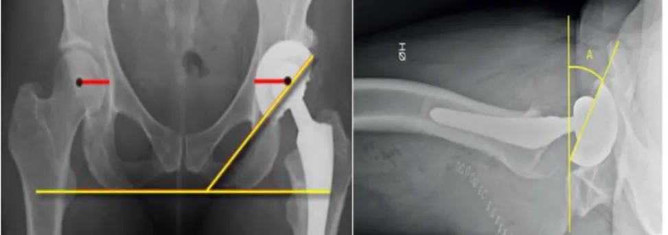
evaluated post-operatively on anteroposterior radiographs29 especially for detecting the inclination angle, or on lateral radiographs and CT scans for assessing the anteversion angle (as this cannot be determined reliably on an AP radiograph62). So, in the radiograph definition (used for CT scans too63), the inclination is the angle between the longitudinal axis and the acetabular axis when projected onto the coronal plane (thus, the angle formed through the face of the acetabulum and the transverse axis) and the anteversion is the angle between the acetabular axis and the coronal plane (Fig.18);

(30)

Fig.18: The upper-left panel shows the inclination angle in a radiograph of an implanted pelvis; the upper-right panel shows a lateral shoot-through radiograph in which A is the anteversion angle; the down panel shows: a. sketched anteversion angle; b. anteversion angle in a CT scan.

• in the operative approach, the inclination angle is defined as that between the acetabular axis and the sagittal plane, while the anteversion is the angle between the longitudinal axis of the patient and the acetabular axis as projected onto the sagittal plane.

The measured average value of the inclination and anteversion angle, conventionally used by clinicians for diagnosis and surgery, are respectively of 45° and 20°29, 30, 31, 64, 65, 66_.

1.3.5.1 The Standard Acetabular Plane

All the previous mentioned reference frames (paragraph 1.2.2) are suitable for an entire pelvis. As in in vitro application hemipelvis is frequently adopted, Morosato et al.24 defined a reference frame suitable for a single hemipelvis, adapting the APP reference frame: this is called Standard Acetabular Plane (SAP) (Fig.10). Due to the link with the orientation of the acetabular plane, it can be potentially used to assess clinical problems67. In addition, the relative alignment of the proposed reference frame with respect to the ISB reference frame was measured. This reference frame born specially to overcome the problem related to the different orientation of the cup in cadaveric specimen. Measuring with respect to the SAP it was possible to standardize the actual alignment.

(31)

31

Fig.19: Visualization of the SAP reference frame

(the picture shows the acetabular component implanted on left hemipelvis, which was potted and painted ad hoc for the Digital Image Correlation analysis).

1.3.6 Failure risks of the Total Hip Arthroplasty

In THA, the causes of failure of primary implant are several. It has been reported 68,69 that the prostheses may fail because of:

• implant fracture,

• surgical technique error, • dislocation,

• wear/osteolysis, • infection,

• periprosthetic fracture,

but especially because of the late aseptic loosening, leading to the revision surgery70 _{(up in the} figure Fig.20, the percentage of revisions, because of the failure of the THA, reported in some registers and studies from 2006 to 2011 are shown; down in the figure, the number and the percentage values of diagnosis in revision of primary THA are reported from the Regional Register of Orthopaedic Prosthetic Implantology (RIPO), which depends on all the orthopaedic units in the Emilia-Romagna region in 2013: the most common cause of revision is the cup aseptic loosening71).

(32)

Fig.20 Up: the percentage of revision because of the failure risks of the THA reported in some registers/ studies from 2006 to 2011; “Current study” refers to Delaunay et. al. study69_{; Down:}

number and percentage values of diagnosis in revision of primary THA are reported from the Regional Register of Orthopaedic Prosthetic Implantology (RIPO).

In general, aseptic (not caused by infection) loosening refers to the failure of fixation at the bone/implant interface, with resultant micro- or macro-motion of the implant, relative to the adjacent bone. It may occur early, because of the failure of initial ingrowth of bone into the prosthesis or caused by poor cementing technique. Alternately, loosening of a fixed implant may occur months (or years) after implantation, potentially because of mechanical overload, physiologic bone resorption, or a combination of both at the bone–implant interface Ref. In addition, aseptic loosening is due to the presence of debris caused by the wearing of the prosthetic

(33)

33

components. The localization in situ of these particles can be the result of inadequate initial fixation, mechanical loss of fixation over time, or biologic loss of fixation caused by particle-induced osteolysis around the implant, oxidative reactions, minor pathogen contaminations ref. When the mobilization affects a significantly large area at the implant-bone interface, then the ingrowth process will result in formation of fibrous or fibro-cartilagineous tissue more than bony tissue: this is the initial anti-inflammatory response of the body. Later the macrophages absorb particles. The osteolysis process act and lead to the failure of the implant (Fig.21). Pain and functional limitation often represent the final phase of this process.

In cemented implant, from radiographic examination,

bone resorption

progressively enlarges lytic foci around the prosthetic components. Mechanical loosening of the device ultimately occurs, occasionally with further fragmentation of the cement surrounding the components72_.

Fig.21: Representation of the Osteolysis process

Similar lytic bone resorption may take place in cementless arthroplasties due to debris produced by wear of the femoral head against the polyethylene acetabular component as previously mentioned (2.6.3).

Thus, the nature of the implant technique (cemented or cementless) influence the rate of loosening: despite its initial stability, cemented implants demonstrate an unfavourable rate of late aseptic loosening. Charnley73 reported a 25% overall incidence of aseptic loosening of cemented acetabular components at 12-15 years. Sutherland et al.74_{reported a 29% rate of loosening at 10} years and underlined that acetabular loosening increased exponentially after 8 years 50_{, causing} more debris then the cementless implants. However, exact rates of aseptic loosening are difficult to define, since definitions and methods of diagnosing loosening vary considerably in the literature.

Recently the AAOS (American Academy of Orthopaedic Surgeons) developed a treatment algorithm for osteolysis as well as several “pearls” of surgery75_{as shown in figure. (Fig.22).}

(34)

Fig.22 Treatment Algorithm developed by the American Academy of Orthopaedic Surgeons75.

1.4 PRIMARY STABILITY

Primary stability is the essential prerequisite to achieve the osseointegration of prosthesis with bone15. The primary stability is the capacity of the prosthesis to not incur in loosening (below a low predetermined threshold) in a conventionally adopted period equal to the first 90 days right after the settlement of the acetabular component.

The stabilization of the cup after the surgical implant is of outstanding importance to create the right environment to favour the osteointegration at the bone-implant interface. There is still not consensus about an absolute definition of the primary stability. Either tested in vivo, in vitro, or detected by clinicians through diagnostic tests, the primary stability can be assessed by mean of different methods. For sure, this is the outcome of both a good osteointegration and of a well performed implant. If the osteointegration is not achieved, the formation of fibrous tissue may occur, in the cup-bone interface, leading to the aseptic loosening 76 (Fig.23).

(35)

35

Fig.23: Flowchart about the influence of Primary Stability on the failure of the implant (if the primary stability is ensured, this yields a good osteointegration).

The osseointegration is the bone ingrowth, where new bone is laid down directly on the implant surface and the implant exhibits mechanical stability77 .

1.4.1 In vivo assessment of tolerance to micromotion

As several definitions and not complete understanding of the mechanism of the osteointegration evolution at the implant surface still doesn’t exist, some in vivo studies have been conducted to assess the primary stability from a biological point of view.

In Sennerby et al.’s work78, titanium implants were inserted into the tibia of rabbits. The osteointegration was then assessed over 3-180 days through optical microscopy and transmission electron microscope:

• At 3 days red blood cells and scattered macrophages predominated at the implant surface after 3 days;

• At day 7 multinuclear giant cells were found at the implant surface protruding into the bone marrow and in areas with no bone-titanium contact;

• At days 14-28 gradually more frequently with longer time, apparently fully mineralized bone was seen close to the implant;

• At days 28-180 the bony tissue is born, and the mineralized bone continue to ingrowth and move to the implant;

(36)

Similarly, Søballe’s work79_{, was focused on the influence of micromovements on bony ingrowth} into titanium alloy (Ti) and Hydroxyapatite (HA)-coated devices, implanted into femoral condyles of seven mature dogs. A loaded unstable device producing movements of 500 micrometers during each gait cycle was developed while a stable device was kept as controls. Histological analysis after 4 weeks of implantation showed a fibrous tissue membrane surrounding both Ti and HA-coated implants subjected to micromovements, whereas variable amounts of bony ingrowth were obtained in mechanically stable implants. Unstable HA-coated implants were surrounded by a fibrous membrane containing islands of fibrocartilage with higher collagen concentration, whereas fibrous connective tissue with lower collagen concentration was predominant around unstable Ti implants. In conclusion, micromovements between bone and implant inhibited bony ingrowth and led to the development of a fibrous membrane.

Obsorn’s and Newesley’s studies showed that the bone ingrowth occurs because of two events. The first is focused on the osteoblasts deposition and the late mineralization which arise in a specific direction: from periphery to the implant; in other words, the bone goes to encircle the implant. The second event happens when the osteointegration is in the opposite direction (from implant to periphery). The apposition of new bone requires a continuous recall of cells from the bone and bloodstream to the implant, since the osteoblasts, after differentiation, are only able to produce bone by apposition. Once they are polarized, they produce extracellular matrix proteins, especially collagen, in order to give a precise structure to the bone-implant interface, which, after calcification, is transformed into an osteoid matrix and finally into bone tissue 80.

The in vivo most relevant result is that: if no micromotions are detected below 20 micrometers, there is not the evidence of fibrous tissue formation; above 150 micrometers, the fibrous tissue formation happens. Between 20 and 150 micrometers both events can occur81, 82.

1.4.2 In vivo assessment of cup stability

A different in vivo approach consists in assess failure of the acetabular component by mean of the stereophotogrammetric analysis. An interesting in vivo study has been conducted by Nieuwenhuijse et al.83 with clinical and Roentgen Stereophotogrammetric Analysis (RSA) for ten years follow-up, establishing the existence of the relationship between the early migration and the late aseptic loosening of the acetabular cups. In fact, early migration, as RSA measured has good diagnostic capabilities for the detection of acetabular components at risk for future aseptic loosening and this method appears to be an appropriate means of assessing the performance of new implant-related changes. The in vivo follow-up showed that after two postoperative years, the loose acetabular components showed markedly greater and more rapid cranial (upper) translation and rotation about antero-posterior axis (change of inclination). Similarly, Kim et al. used the Ein-Build-Rontgen-Analyse (EBRA-cup) to prove that the absence of proximal translation within the first 60 months indicates a component is not likely to be loose. _{Both the EBRA-cup and the RSA} are two technique which improves the accuracy of radiographic (clinical) criteria 84,85.

(37)

37

So, follow-up tests 83,86,31, 87, combined with clinical criteria assessments, indicate some thresholds values, such as (Tab.2):

Tab.2: Thresholds values for cranial migration of the acetabular cup (mm) and variation in inclination (°) in literature.

about change of inclination and along cranial translation (Fig.24).

Fig.24 outline of the change of inclination and the cranial translation of the cup.

1.4.3 In vitro assessment of cup stability

In vitro tests are conducted to measure the motion of the acetabular component in different loading

conditions and different models are used.

1.4.3.1 Simplified assessment methods

Some studies have been developed simulating the acetabular cavity by mean of a simplified way: in foam blocks with a controlled density15,56_{. Static load to failure may be applied (torsional, edge} loading and pull out tests88,87, 68,89_{), for essentially investigating the design limits of the implant to} extreme conditions90.

CRANIAL MIGRATION VARIATION IN

INCLINATION

Nieuwenhuijse et al. 1.76 mm 2.53°

Abrahams et al. 3 mm 5°

Kim Y.S et al. 1 mm 1.15°

(38)

1.4.3.2 Realistic assessment methods

To better simulate physiological conditions, other studies apply cycles of load until failure or for a fixed number of cycles and by using animal and cadaveric specimens 50,55, 91,58,26,

Two representative in vitro studies are the ones by Perona et al. 50 and Kwong et al.55

Perona’s study was designed to quantify initial micromotion at the cup-bone interface and to have a comparison between different fixation methods (cemented, cementelss, with screws and without). To measure the displacements, they used current transducers (Fig.25). Relative motions between the cup and the bone, perpendicular to the plane of the rim, were able to detect, during 5 cycles of axial loads of up 2534N, reaching 3 times the bodyweight (if 80 kg person).

Fig. 25 Focus on Eddy current transducers on the cadaveric specimen.

The average micromotion at the maximum applied load were 162 micrometers at the ilium, 97 micrometers at the pubis, and 54 micrometers at the ischium, with the press fit fixation.

Kwong et al. conducted a similar study using exstensometers fixed to the specimen with a custom setup(Fig.26).

(39)

39

They evaluated the performance of the press fit fixation, testing (with axially load) the acetabular cup implanted in cadaveric specimens simulating a critical physiological load (in a single leg stance) with or without the presence of screws (Fig.27).

Fig.27: Results in Kwong et al’s work.

Thus, in vivo tests underline the importance of keeping micromotions at the bone-implant interface below a threshold (still not conventionally decreed), because it is a fibrous tissue formation index52. Thus, the in vitro tests on acetabular components are conducted for preclinical primary stability assessment, because it is extremely important to have an early performance on these kinds of implants to prevent mechanical failure or to investigate what is the best method of implant (with screws or not, with or without cement and so on) or eventually a design variation.

1.4.4 In silico assessment of cup stability

No studies about the assessment of the primary stability have been carried out in silico yet. Despite this, an explicative example about FE analysis has been conducted by Gosh (2012), who used the Digital Image Correlation technique to validate a FEM predicting strain distribution both for the intact and implanted hemi-pelvis (with the THA acetabular component).

FEM was a valid predictor of the strain distribution, advantageous for detecting full field data and to allow investigations of many variables quickly and relatively inexpensively92.

(40)

1.4.5 How to measure the primary stability of acetabular cups: Clinical criteria

Clinicians usually assess the primary stability through the evaluation of the aseptic loosening. The diagnosis relies especially on clinical symptoms and on radiographic criteria.

The challenges in diagnosis arise from the difficulty in detecting the presence of implant motion, particularly when it is in the submillimeter range. Thus, qualitative measures, such as radiolucent lines adjacent to implants or increased absorption on radiographs, are typically used, together with the assessment of the pain.

Clinicians are used to act a differential diagnosis: firstly, they evaluate the origin and the localization of the pain. In a follow-up study (about the diagnosis of the dislocation)93 , authors use the Postel Merle d’Aubigne scoring, showed in Fig.28, that in 1954 was published to give a rating scale both to the intensity of the pain and to the activity which leads the pain to raise.

Fig.28: Scoring Pain with respect to mobility and ability to walk.

By scoring the pain it is possible to speculate about the severity of the case, as a first approach during this phase of anamnesis and objective examination. Then a standard protocol is followed:

1. clinicians assess if there would have been a pain change due to extrinsic causes, not inherent with the surgery;

2. if it is found that there was an interval without pain after operation, it is necessary to consider prosthesis intrinsic causes instead of extrinsic causes:

3. RX, PCR (Protein C Reactive, index of inflammation if the test is positive) and ESR (Erythrocyte Sedimentation Rate, index of inflammation if the test is positive) investigations are necessary;

4. if PCR and VES are negative, the diagnosis must continue with the bone scan: if this is positive, clinical assessment suggest aseptic loosening. Conversely it suggests other causes;

(41)

41

5. if PCR and VES are positive it probably deals with infection (Fig.)94.

Radiographic criteria include measuring acetabular component migration relative to surrounding bone, identifying radiolucent lines 95. A radiolucent line is a dark line of demarcation between the acetabular component and the cancellous bone. According to DeLee and Charnley, in case of radiolucent lines with a thickness ≥ 2.0 mm, or in any zone with the presence of sclerotic border, the implant is considered loose. A sclerotic border is defined as a condensed bright light adjacent to the surrounding cancellous bone 83. However, the accuracy and interobserver agreement of these measures are unknown 96.

Another clinical aseptic loosening parameter is the visual identification of the cup migration. This assessment relies on the observation of a series of radiographs or of scintigraphy too, which is generally used to detect inflammations or tumours.

With the presence of loosening, the scintigraphy shows areas of anomalous hyperconcentration of the radiopharmaceutical perfusion, in the bone around the prosthesis.94.

Sensitivity Specificity

Scintigraphy 83% (confidence interval 95%, 69-92) 67% (confidence interval 95%, 46-84)

Radiography 85% (confidence interval 95%, 71-94) 85% (confidence interval 95%, 66-96)

Tab.3 Sensitivity and Specifity of scintigraphy and radiography developed by Temmerman OP et al.’s follow-up study97_.

Among the techniques above, as shown in Tab.3., the radiographic analysis has the higher accuracy (and the lowest risk) in detecting the loosening of the cup, hence in evaluating the presence (or not) of the primary stability.

All these methods are limited by the inter-observers’ variation and the possibility of a loosening not detectable on radiographs of the diagnostic tests.

The pain parameter is such a controversial tool, too. It may range from no pain to persistent hip pain beginning immediately after THA or even later (many months or years after a previously nonsymptomatic THA).

These limits underline the importance of preclinical assessments of the implant stability, that are quantitative and reliable. To reach this goal many studies are conducted in vivo, in silico and in

vitro.

(42)

1.5.1 Displacement sensors

Displacement transducers measure the position throughout an electrical signal variation. The Linear variable differential transformer (LVDT) is a type of electrical transformer used for measuring absolute linear displacement (position).

An LVDT consists of a coil assembly and a cylindrical ferromagnetic core with a probe at the apex which feel the displacement of a specimen (Fig.29). The coil assembly consists of three coils of wire wound around the hollow form. The core can slide freely inside the form. The centre coil is the primary coil, which is excited by an AC source as shown (Fig.29) (The frequency is usually in the range 1 to 10 kHz98). The magnetic flux produced by the primary is coupled to the two secondary coils, inducing an AC voltage in each coil. In fact, as the core moves, these mutual inductances change, causing the voltages induced in the secondaries to change. The coils are connected in reverse series, so that the output voltage is the difference (hence "differential") between the two secondary voltages. When the core is in its central position, equidistant between the two secondaries, equal but opposite voltages are induced in these two coils, so the output voltage is zero. Thus, the core displacement is transduced in voltage values.

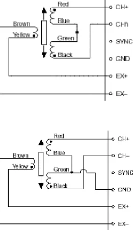
Fig.29: On left, LVDT design with focus on the probe; on right general LVDT assembly.

The magnitude of the output voltage is proportional to the linear displacement of the core (up to its limit of travel). The phase of the voltage indicates the direction of the displacement. When stated without a polarity, it is called LVDT’s full range, full stroke, or total stroke.

By mean of wire connections, the LVDT is commonly connected toa signal conditioning circuit that translates the output of the LVDT to a measurable voltage.

The wire connection can be at 4-wire or 5-wire configuration (Fig.30) and the respectively equations that relate displacements with voltage, are: