Microscopic Dynamics of Polymer Melts: Numerical Simulations with Coarse-Grained Models

University of Pisa

”Galileo Galilei” PhD School

Applied Physics

Ph. D. Thesis

Microscopic Dynamics of Polymer

Melts:

Numerical Simulations with

Coarse-Grained Models

Oleksandr Chulkin

Advisor: Prof. Dr. Dino Leporini (University of Pisa)

Introduction

Every liquid in principle can transform into a glass if it is cooled or compressed fast enough. Glass is one of the most important artificial materials utilized by man. Numerous applications of glass materials and glass transition phenomenon include obtaining of the optimal wet-skid resistance by using the tread rubber with high glass transition temperature [1, 2], enhancement of the ballistic pen-etration resistance of armor coatings obtained by energy dissipation associated with an impact-induced transition of the coating to the glassy state [3, 4], the material selection for acoustic tiles on submarines allowing to undergo the glass transition at the frequency of the active sonar at seawater temperatures thus dampening the sonar [5], arterial walls restoring[6], preservation of food [7, 8, 9], highly soluble pharmaceuticals [10]. So, the study of glassy state tends to be one of the most promising and interesting tasks in chemistry in our days. This fact was my main motivating factor to study the structural and dynamical char-acteristics of the polymer melt approaching to glass transition from above in group of Prof. Dino Leporini in Pisa University.

The particles(in this Thesis the word “particle” signifies the most elemen-tary rigid part of the system under investigation. In general, it can be either molecule for the system containing the rigid molecules, or atom for the case of flexible molecules. As far, as in this Thesis the polymer melt is the system that I am investigating, the word “particle” in context of my research signifies the monomer) spend increasing periods of time, rattling in cages formed by their neighbors while the liquid, consisting of these particles, approaches the glass transition. Finally, the particles are relaxed from their cages - this process is called the structure relaxation. The main aim of this thesis is the investigation of the microscopic dynamics of the particles trapped in these cages and the study of the possible ways to connect this fast dynamics in cage to slow macro-scopic dynamics associated with structure relaxation. First direction of research is based on the density-temperature scaling of the one of the most important characteristics of the cage dynamics - the Debye-Waller factor(that is the ampli-tude of the particle’s rattling in the cage, see the section 1.2 for the details). The density-temperature scaling has become very popular in the recent years due to the improvement of the technical equipment of the experiments, that allowed to change both density and temperature of the system in simultaneous and prompt way. The density-temperature scaling of the structure relaxation time for single and multi-component liquids having different interaction potentials was intro-duced and investigated in this thesis from the different points of view, including the pressure-energy correlations and potential energy landscapes with citations of the correspondent sources (see the section 3.1). Recent research of the Prof. Leporini group[11] has presented the universal scaling between the structure re-laxation time and Debye-Waller factor(see the subsection 3.1.5). Nevertheless, the research of the density-temperature scaling of the Debye-Waller factor has been missing so far and I tried my best to improve this situation and to show that the density-temperature scaling is valid for the microscopic processes, too. In the terms of the second direction of investigation I studied several functions of cage correlation for the polymer melt. This study should have allowed me to better understand the processes taking place in the cages or “shells” surround-ing the tagged particle and to discover the new types of connection between these microscopic processes from one side and the macroscopic processes, like

e.g. the structure relaxation, from another side. Results of this study could help to develop the new ways of understanding of the universal scaling between the structure relaxation time and Debye-Waller factor. Furthermore, it is in-teresting to study the cage correlation functions of the polymer melt because the polymers have been never studied in this way so far. Previous researches of the correlation functions dealt with the binary mixtures[12], hard spheres and disks[13], etc. I also have to say that this study is based on introduction of different correlation functions including the self-correlation functions of dis-placement that have not been studied in context of the liquids state research so far.

As to the meaning of the results of the thesis, I may state the following:

• the density-temperature scaling of the Debye-Waller factor is evidenced(see

the section 3.1 and the Chapter number 4). The values of the scaling exponent γ are consistent with the predictions from the study of Lennard-Jones liquids. Data of all the polymers in the study, that have different molecular masses and interaction potential, collapse the straight lines of Debye-Waller factor vs T Vγ _{plot, where any straight line is uniquely}

de-fined by the molecular mass and parameters of the interaction potential. These lines cross in one “universal” point.

• the cage correlation functions, describing the time evolution of the

neigh-bor cage of the given particle(see the subsection 3.2.1 and section 5.1) and following from the immediate physical interpretation, represent the alternative but perfectly equivalent instrument for the description of the structure relaxation, compared to the more rigorous intermediate scatter-ing function.

• the analysis of the spatial correlation of displacement(see the subsection

3.2.2 and section 5.2) evidences the link between the well-known static properties of the system and the dynamic properties, represented by the direction and modulus correlation functions of displacement. Origin of this correlation is not perfectly clear and needs further investigation.

• analysis of the time correlations of displacement (see the section 5.3) shows

that the directionality of motion rather than the displacement modulus seems to connect the fast microscopic and slow macroscopic dynamics. The direction of the displacement of a particle at the time scales of cage regime determines in general the direction of the particle’s motion even at much longer times.

As far, as the outlook of the Thesis is concerned, I have to point out that the further investigation, generalization and improvement of these results could be useful. The results of current Thesis allow to construct only several very narrow and rickety bridges between the fast microscopic and slow macroscopic dynamics. These narrow links should be united with the other existing ones and with those that will be created in future, thus forming the new theories, methods and approaches. Among the possible ways of developing of the results of this Thesis I can point to either the prospect of the study of the influence of T Vγ on the behavior of the cage correlation functions, uniting the two main directions of research of this thesis, could be the most promising direction of further study, or to the aforementioned possible research of the reasons of the

correlation between the static and dynamic(represented by the direction and modulus correlation functions of displacement) properties of the system. Results and outlook of the Thesis are discussed in the Conclusions in more detailed way. My thesis consists of five chapters. First chapter of my PhD thesis presents the introduction to glass transition phenomenon (section 1.1); covers the in-formation about the static structure and relaxation in liquids and introduces the functions that describe these processes (section 1.2); and describes the glass transition in polymers with particular attention to the similarities and differ-ences of the glass transition processes in simple liquids and polymers(section 1.3), thus explaining why the polymers usually are the good glass-formers.

Then, in the second chapter, covering the methods of the computer simula-tions of polymers, there follow:

• the review of numerous methods of molecular dynamics and (a bit) of

monte-carlo simulations of the glass-forming polymers(section 2.1), allow-ing to better understand the future ways of development of the simulation studies of the polymers and to enrich the arsenal of a modern scientist with new powerful computational methods enabling the simulations to become more quick and effective

• separate section (2.2) describing the numerical methods and MD model

(developed by Cristiano De Michele, a former member of the Leporini group) used in the MD simulations runs during the work over the fourth and fifth chapters

Third chapter contains the theoretical background for the fourth and fifth chap-ters.

• the theoretical introduction to the popular aspect of density-temperature

scaling of the relaxation time in numerous classes of simple liquids and polymers (section 3.1). Theoretical basis of the scaling and its connec-tion to the inverse power law is discussed in the subsecconnec-tion 3.1.1, the numerous ways of approximation of the scaling exponent γ are presented in the subsection 3.1.2. The speculations upon the relation between the density-temperature scaling and the pressure-energy correlations in liquids are presented in the subsection 3.1.3; the connection of the temperature-density scaling to the fragility and potential energy landscapes is discussed in the subsection 3.1.4. Section ends with results of Leporini group (sub-section 3.1.5) obtained just before beginning of my work over the PhD thesis. These results allowed to ascertain the universal scaling between the fast microscopic and the slow macroscopic dynamics and also urged me to explore the possibility of temperature-density scaling not only of the slow macroscopic dynamics reflected in such macroscopic parameter as the relaxation time, but also of the microscopic dynamics closely connected to the Debye-Waller factor.

• section 3.2, consisting of the introduction to the functions regarding the

cages surrounding the tagged atom (subsection 3.2.1) and the basic the-oretical information about the spatial correlation functions (subsection 3.2.2)

The original results of the research of temperature-density scaling of the Debye-Waller factor are presented into the fourth chapter.

The fifth chapter reports an original investigation of the correlation functions of supercooled polymeric melt. The peculiarities of motion of the atoms in the supercooled liquid, especially when it approaches the glass transition, are always of great interest and importance, because the understanding of the laws of this motion could be crucial for prediction of various properties of materials close to their glass transition. The correlation functions give us a rather detailed picture of the motion of the atoms. In the section 5.1 I explored the correlation functions regarding the cages surrounding the tagged atom. The description of the program, calculating the neighbor list and cage correlation functions (already introduced in subsection 5.4.1), follows in subsection 5.1.1. The results of the run of this program using the input data from the simulations of our MD model, already described in section 2.2, are presented in subsection 5.1.2. In section 5.2 there follows the research of the spatial correlation functions. The structure of this subsection is similar to the previous one with the introductory part of the corresponding functions being presented in subsection 3.2.2, program description in subsection 5.2.1 and the results of the run in subsection 5.2.2. In the section 5.3 I introduced the original self-correlation functions of displacement in subsection 5.3.1. The program, calculating these functions, is described in the subsection 5.3.2, the results of run - in the subsection 5.3.3.

CONTENTS

1. Chapter 1. Glass transition in simple liquids and polymers.

Phenomenol-ogy and experimental characterization (differences and similarities) . . 9

1.1 Introduction to the glass transition phenomenon . . . 9

1.2 Static structure and relaxation in liquids . . . 11

1.3 Introduction to glass-forming polymers. Differences and similar-ities between the glass transition of simple liquids and that of polymers . . . 16

2. Chapter 2. Molecular dynamics simulations of polymers . . . . 21

2.1 Computer simulations of polymers and polymer glasses . . . 21

2.1.1 Quantum level . . . 22

2.1.2 Atomistic level . . . 23

2.1.3 Mesoscale level . . . 32

2.1.4 Continuum level . . . 36

2.1.5 Multiscale level . . . 38

2.2 Numerical methods and simulation protocol used in the work . . 45

2.2.1 Force field . . . 45

2.2.2 Statistical ensembles . . . 46

2.2.3 Algorithm . . . 46

2.2.4 Simulation protocol . . . 46

3. Chapter 3. Main theoretical results used in the following: introduction to the density-temperature scaling, introduction to the cage correlations 49 3.1 Temperature-density scaling of relaxation time and Debye-Waller factor. Theoretical background . . . 49

3.1.1 Temperature-density scaling of polymeric and non-polymeric glassformers. IPL . . . 49

3.1.2 The scaling exponent approximation.Gr¨uneisen parameter 53 3.1.3 Pressure-energy correlations . . . 55

3.1.4 Potential energy landscape. Fragility . . . 58

3.1.5 Universal scaling between the fast microscopic and the slow macroscopic dynamics . . . 62

3.2 Cage and spatial correlations . . . 63

3.2.1 Introduction to cage correlations. Definition of the neigh-bor list and cage correlation functions . . . 63

3.2.2 Theoretical background to the spatial correlations of dis-placement. Definition of the displacement correlation func-tions . . . 66

4. Chapter 4. Temperature-density scaling of relaxation time and

Debye-Waller factor. Original work and results . . . . 69

5. Chapter 5. Cage correlations. Original work and results . . . . 81

5.1 Neighbor list and cage correlations . . . 81

5.1.1 The program CageCorrelation.c . . . 81

5.1.2 Analysis of the simulations . . . 81

5.2 Spatial correlations of the displacement . . . 86

5.2.1 The program MotionCorrelation.c . . . 86

5.2.2 Analysis of the simulations . . . 86

5.3 Time correlation of the displacement . . . 92

5.3.1 Definition of the self-correlation functions . . . 92

5.3.2 The program MotionCorrSelf.c . . . 93

5.3.3 Analysis of the simulations . . . 93

6. Conclusions . . . . 97

7. Appendix. Statistical methods used . . . 101

7.1 Pearson’s correlation coefficient . . . 101

7.2 Root mean square error . . . 101

7.3 Pearson’s χ2test statistic . . . 101

1. CHAPTER 1. GLASS TRANSITION IN SIMPLE LIQUIDS

AND POLYMERS. PHENOMENOLOGY AND

EXPERIMENTAL CHARACTERIZATION (DIFFERENCES

AND SIMILARITIES)

In this chapter I recount the glass transition phenomenon (section 1.1), cover the information about the static structure and relaxation in liquids, presenting the functions that describe them (section 1.2), and introduce the glass-forming polymers, whose glass transition is somewhat different from non-polymeric ma-terials (section 1.3).

1.1

Introduction to the glass transition phenomenon

Glass transition takes place when simple liquids [14], polymers[15], bio-materials[16], metals[17],[18] and molten salts[19] are cooled or compressed fast enough to avoid crystallization and, finally, are freezed into a non-crystalline solid-like state - a glass. The glass transition does not have a well-defined transition tem-perature and it is not a phase transition [20]. Any liquid is able to form a glass if it is cooled fast enough [21]. Hence, the glassy state may be regarded as the fifth state of conventional matter: glass is solid as the crystalline state but isotropic and without long range order as the liquid state [22]. The particles spend some periods of time rattling in the cages formed by their neighbors; and these pe-riods increase while approaching the glass transition. Finally, if the system is not vitrifying(otherwise there happens the structural arrest), the particles are relaxed from these cages. The period of time that is required to reorganize the topological structure of the liquid and to allow the kinetic unit to escape from the cage is called the structural relaxation time τα. The dynamics of the

super-cooled liquids and the relaxation processes is very complex. One of the most important features of this slow dynamics is the dynamic heterogeneity[23, 24]: in the same environment and same moment of time some molecules could be characterized by fast motions with others being much slower, acting as cages for the faster. This picture is dynamic because in just few moments (usually on the time scale of τα) the fast molecules could become slow, due to the mutual

interactions, and vice versa. Fast and slow molecules are usually clustered in domains. The sizes of these domains are assumed to be of the order of several nm [25, 26, 27, 28].

Angell plot [29] shows the correlation between the temperature decrease towards the glass transition temperature Tg and the corresponding increase of

the logarithm of relaxation time. Tg is obtained by definition when liquid is

cooled enough, so that its ταis equal to 100 seconds [29]. The reproduction of

the Angell plot(viscosity versus Tg

T ) is shown in the Figure 1.1. For the so-called

“strong” liquids the dependence of τα on normalized Tg

Fig. 1.1: Angell plot(reproduced from [29]) of the viscosity against Tg/T in log-scale.

Based on the experimental data. η is the viscosity, τα is the relaxation

time,Tg is the glass transition temperature, T is the temperature. In this

representation, strong glassformers such as SiO2 give straight lines, while

the fragile glasses (for example, OTP) exhibit the strongly curved plots. The hydrogen-bonded materials, like glycerol, correspond to the moderately curved plots.

liquids are represented by the straight lines at the Figure 1.1. Strong liquids exhibit the so-called Arrhenius temperature dependence:

τα= τ0exp(

∆(E)

kBT

) (1.1)

where ∆(E) is the free energy of activation (of a flow event) and τ0is a constant.

The so-called “fragile” or “super-Arrhenius” liquids have higher radius at the Angell plot, hence they do not exhibit the Arrenius-like behavior. The structure relaxation time of such liquids is well approximated by the empirical Vogel-Fulcher-Tammann-Hesse expression, obtained from the experiments with fragile glasses [30], [31]:

τα= τ0exp[

A

T− TV F] (1.2)

where τ0 is the high temperature limit of relaxation time, TV F is the

Vogel-Fulcher temperature which indicates the divergence of the relaxation time at infinite viscosity, corresponding to the complete blocking of the structural re-laxation, A is the strength parameter whose value is related to the degree of de-viation of the τα(T ) curve from the Arrhenius equation (see the Figure 1.1)[32].

Typically, for a fragile system A is rather small (down to about 3) and for strong one is essentially higher (up to about 100). Fragility is another interesting pa-rameter of the glass-forming liquids. It is defined as follows[33]:

mv= ∂log(η)

∂(Tg

T )

The van der Waals molecular liquids (like OTP) are the classical fragile (mv=

70÷ 150) systems. The strong glass-formers (mv = 17÷ 35) are character-ized by strong covalent directional bonds, forming space-filling networks (like silica). Hydrogen bonded materials (like glycerol or propylene glycols) demon-strate the intermediate levels of fragility (mv = 40÷ 70). The

experimen-tal evidences demonstrate the complex behavior of temperature dependence of the structural relaxation time. Actually, there are several experimental and numerical simulation results [34, 35, 24, 36] supported by the theoretical studies[37, 38, 39, 40, 41, 42] that reported that the slowing down of the dy-namics on approaching the glass transition temperature and the increase of the free energy of activation could be related to the onset of cooperative motions, involving molecules on an increasing correlation length .

While speaking about the relation of glass transition and cooperative motion, it is very difficult to omit the the Adam-Gibbs(AG) model[37]. The AG model is one of the most popular ones that try to explain the increase of free energy of activation while approaching to glass transition from above and to link it to the size of the cooperative regions. According to this model the increase of

τα of the glass-forming systems is linked to the increasing size NCRR of the

cooperatively rearranging regions (CRR). The AG model postulates that the free energy activation barrier for a CRR relaxation is linearly increasing with

NCRR, that, in turn, is the reverse of configurational entropy Sc of the system.

So, the reduction of Sc on approaching the glass transition is connected to the

slowing down of structural dynamics, according to the equation:

τα(T, P ) = τ0exp[

Cag T Sc(T, P )

] (1.4)

where τ0 is the value of ταin the limit of infinite T Sc, and Cag = (s∗c∆µ/R). R

is the gas constant (R≈ 8.314 J mol−1K−1). s∗_c = kBln 2 and ∆µ is the free

energy activation barrier for an elementary transition, i.e. at high temperatures where cooperativity does not take place and NCRR = 1. In recent years the

Equation 1.4 has been applied to reproduce the dynamics of supercooled liquids above the glass transition in different cases[43, 44, 45, 46]. It is interesting, that, if Sc can be expressed in terms of a first order polynomial of 1/T , the

Equation 1.4 transforms into the Vogel-Fulcher-Tammann-Hesse expression (see the Equation 1.2) for τα(T ).

1.2

Static structure and relaxation in liquids

There is a set of functions helping to describe the relaxation process and the static properties. First of all, let us speak about the main function describing the static properties of a liquid - the radial distribution function. The radial distribution function, g(r), is the probability to find a particle at distance r if there is a particle at zero distance [47, 48]:

g(r) = V

2

N2n

(2)_{(r) (1.5)}

where N is the total number of particles in the system, V is the volume of the system, n(2)(r1, r2)dr1dr2is proportional to the probability of finding a particle

is a particle in a volume element of radius dr1 with center in r1 irrespective

of where the remaining particles are [47]. For isotropic liquid g(r) linearly depends on r. The value of 4πρr2g(r)dr defines the number of particles located

between the spheres with center at given particle(r = 0) having the radii of r and (r + dr), respectively. Hence, the probability to find a particle at distance not smaller than r and not larger than r + dr from the given particle is defined equal to 4πρr2_Ng(r)dr. In the Figure 1.2 there is shown the typical form for the

g(r) dependence on r. At low r g(r) = 0 due to repulsion of the atoms. At a

distance roughly equal to the atomic diameter, there is a pronounced peak in

g(r), which denotes a sphere or “shell” of nearest neighbors. At higher values of r there are oscillations representing more distant neighbors. These oscillations

decrease in amplitude with increasing r, and eventually g(r) approaches the (unit) mean density of the system[47].

0 1 2 3 4 5 6 7

r

g(r)

Fig. 1.2: Typical form of the radial distribution function g(r), obtained from the

molec-ular dynamics simulation of dimer. The interaction potential parameters are (p, q) = (6, 10), the volume V = 0.968, the same temperature T = 0.5 (see subsection 2.2 for details on the density and temperature units) .

The microscopic particle density ρ(r) is defined as follows:

ρ(r) = N

∑

j=1

δ(r− rj) (1.6)

where δ(r) is the Dirac delta-function and rj are the positions of the particles.

The static structure factor S(q) can be defined as [48]:

S(q) =⟨1

Nρqρ−q⟩ (1.7)

where ρq is a Fourier component of the microscopic density:

ρq = ∫ ρ(r) exp(−iq · r)dr = N ∑ j=1 exp(−iq · rj) (1.8)

where q is the difference between the wave vectors of incident and scattered radiation and ρ.

Wave vector is defined as follows:

q = 2π

λ (1.9)

where λ is the wavelength. So, we can rewrite the Equation 1.7 as:

S(q) =⟨1 N N ∑ l=1 N ∑ j=1 exp[−iq · (rj− rl)]⟩ (1.10)

We can express the static structure factor as the Fourier transform of the g(r):

S(q) =

∫

V

exp(i−→q · −→r )[g(r)− 1]dr (1.11) with −→q being the difference between the wave-vectors of incident and scattered

radiation in neutron time-of-flight measurements. g(r) and S(q) describe the static properties of the liquid. To account for the dynamic properties, let’s introduce the van Hove function G(r, t) [48]:

G(r, t) =⟨1 N N ∑ i=1 N ∑ j=1 δ[r− rj(t) + ri(0)]⟩ (1.12)

The expression G(r, t)dr is equal to the number of particles j in a region dr around a point r at time t given that there was a particle i at zero time and zero distance. The van Hove function can be defined as a sum of its self and distinct parts. The division into self and distinct parts corresponds to the possibilities that i and j may be the same particle or different ones. The self part of the van Hove function is calculated as [48]:

Gs(r, t) =⟨ 1 N N ∑ i=1 δ[r− ri(t) + ri(0)]⟩ (1.13)

while the distinct part looks like[48]:

Gd(r, t) =⟨ 1 N N ∑ i=1 N ∑ j=1,j_̸=i δ[r− ri(t) + ri(0)]⟩ (1.14) If t = 0, then: G(r, 0) = δ(r) + ρg(r) (1.15) where g(r) is radial distribution function, ρ is a numerical density (number of particles per a volume unit). Furthermore:

Gs(r, 0)≡ δ(r) (1.16)

and:

Gd(r, 0)≡ ρg(r) (1.17)

S(q) reaches its maximal value at q = qmax. The qmax is about 2π_a , where a

is the average distance between the neighboring particles (please, compare this condition to the Equation 1.9). The structural relaxation is described by the self

part of intermediate scattering function(ISF) Fs(qmax, t) [48],[49]. Fs(qmax, t)

is the space Fourier transform of the self part of van Hove function Gs(r, t): Fs(q, t) =

∫

Gs(r, t)exp(−iq · r)dr (1.18)

The structure (or α) relaxation time τα is defined as follows [11]:

Fs(qmax, τα) = e−1 (1.19)

Please, see in the Figure 1.3 the example of Fs(qmax, t) with indication of τα.

The plot of Fs(qmax, t) consists of three main parts - the initial decay before the

Fig. 1.3: Fs(qmax, t) dependence on logarithm of time, obtained from the molecular

dynamics simulation of trimer, (p, q) = (6, 10), V = 0.968, T = 0.5. τα is

indicated as according to the Equation 1.19.

big central plateau, the plateau itself, and the long-time decay after the plateau. The initial decay of Fs(qmax, t) plot reflects the effect of ballistic motion. Plateau

itself exhibits the caging effect of the neighboring particles. Between plateau and the initial decay of Fs(qmax, t) there takes place the secondary or β-relaxation,

[50]. After the plateau there comes the α-relaxation [51], that causes the mono-tonic decrease of Fs(qmax, t). In the Figure 1.4 we may observe the q-dependence

of the Fs(q, t) where q changes from small value q << qmax ( λ from the

Equa-tion 1.9 is high, hence this case corresponds to large scale relaxaEqua-tion and high relaxation time) through q = qmax(value corresponding to structural relaxation

time τα) to comparably high value q >> qmax(λ is low, hence the relaxation

scale and the relaxation time are small). The aforementioned α-relaxation is well approximated by the Vogel-Fulcher-Tammann-Hesse expression, see the Equation 1.2 In contrast to α-relaxation, β-relaxation exhibits Arrhenius-like behavior , see the Equation 1.1. And also we have to mention that since the α-relaxation is not Arrhenius-like, it also is not-exponential. In this statement we imply that the normalized relaxation function does not exhibit the exponential behavior[52]:

Φq(t)= exp[−( t τ)

Fig. 1.4: Fs(q, t) plots for different values of q - the wave vector number. Black curve

corresponds to q = 4.5, red - to q = qmax = 7.18, green - to q = 10.5.

Obtained from the molecular dynamics simulation of trimer, (p, q) = (6, 10),

V = 0.968, T = 0.5.

with 0 < βK < 1, called as the Kohlrausch exponent[53], τ being a constant.

The long-time decay of the Fs(q, t) is fitted with the help of the law described by

the Equation 1.20 [54] (called the “stretched-exponential” law). The normalized relaxation function Φq(t) may be calculated , for example, from the inelastic

neutron scattering [52]:

Φq(t)=

Fs(q, t)

S(q) (1.21)

or from dielectric spectroscopy: Φq(t)=

ϵ− ϵ(t)

ϵ− ϵ(0) (1.22)

The recent researches in this field [55] showed strong interconnection between α and β relaxations in their relaxation times and also in other various properties. Stevenson et al. [42] claimed that secondary relaxation is universal (although that is not supported by some experimental investigations[56]) and depends on the configurational thermodynamics of the system. Roland in [57] argued that

β-relaxation is the precursor of the glass transition at the short time scale.

To characterize the fast dynamics of the system behavior near the glass transition we use the mean square displacement(MSD), that has the following definition:

⟨r2_{(t)⟩ =} ⟨

∑N

j=1[rj(t)− rj(0)]2⟩

N (1.23)

where the sum runs over the total number of N monomers, rj(t) is the position

of j-th monomer and the brackets denote a suitable ensemble average. As we have already mentioned in the section 1.1, the closer liquid approaches the glass transition, the greater time it spends to relax its structure. From the microscopic point of view this means that the kinetic unit spends some period of time rattling inside the cage formed by its closest neighbors. This time increases while the system approaches the glass transition. The rattling is characterized by the

amplitude √⟨u2⟩, a quantity similar to the Debye-Waller factor measured in

neutron or light scattering experiments at the picosecond time scales. In our case of MD simulation the Debye-Waller factor is calculated as√⟨r2_(t∗₎⟩ where

t∗ = 1.022 is the inflexion point of log(⟨r2(t)⟩) vs log t [58, 11]. Please, notice that in our simulations t∗∼= 1÷ 10ps [58]( see Appendix A). This is consistent with the time scales of the experimental measurement of the DW factor, e.g. see [59]. The ballistic regime corresponds to the free motion before the particles begin to collide with the other particles thus trapping into the cages. In this region the mean square displacement is well approximated by the following power law:

⟨r2_{(t)⟩ ∝ t}2 _(1.24)

The repeated collisions with the other particles slow the displacement of the tagged one. This process is characterized by a knee of MSD at t∼ √_Ω12

0 where Ω0

is an effective collision frequency, or, in other words, the mean small-oscillation frequency of the particle in the potential well produced by the surrounding ones kept at their equilibrium positions [60]. Successively, the plot of ⟨r2_(t)⟩

(see the Figure 1.5) exhibits the quasi-plateau regime. This is visible more clearly with temperature decrease and/or with density increase. The quasi-plateau regime indicates the time interval corresponding to occurrence of the caging process. At times longer, than τα, for the polymers with chain length

more than 3 there takes place the sub-diffusion or Rouse regime (because of the increased connectivity[61]), formulated as follows:

⟨r2_{(t)⟩ ∝ t}0.5÷0.6 _(1.25)

and after there occurs the diffusion regime, having the following formula:

⟨r2_{(t)⟩ = 6Dt (1.26)}

with D being the diffusion constant. In the Figure 1.5 we see the comparison of the ⟨r2(t)⟩ for dimer and pentamer having the same interaction potential, density and temperature (see the caption). We may notice that the plot corre-sponding to the dimer case consists of 3 regimes - ballistic, plateau and diffusion, while for pentamer there also exists the sub-diffusional regime between plateau and diffusional ones.

1.3

Introduction to glass-forming polymers. Differences and

similarities between the glass transition of simple liquids and

that of polymers

Polymer melts are bulk liquids consisting of macromolecules [62]. These macro-molecules are made up by repetition of fundamental units, called monomers, connected by covalent bonds [63], [64], [65], [66]. Polymer types can be dis-cerned by means of topology and chemical composition. Chain, star, ladder or network are only few structures that can be found in nature. The simplest, the most fundamental and the most often studied form of polymer is a chain or a homogeneous linear polymer. Its length N may be large. N typically ranges between 103and 105 in experimental studies of polymer melts [62] and simula-tions [67], [68]. The chain has an open structure that is strongly permeated by other chains in the melt [64]. This fact has a great impact on the properties of the melt. The monomers pack in a dense way, thus leading to:

Fig. 1.5: The mean square displacement dependence on temperature with indication of t∗and τα. Debye-Waller factor determination. Obtained from the molecular

dynamics simulation. Red curve corresponds to dimer, violet - to pentamer. Both cases have the same interaction potential (p, q) = (6, 12), the same volume V = 1.099, the same temperature T = 0.7

• an amorphous short range order on a local scale • a low compressibility of the melt on a global scale

Both these features are the characteristic of the liquid state. A long polymer in a three-dimensional melt is not a compact. It is a self-similar object with fractal structure [64], [65], [66], so the other chains may penetrate into the volume defined by its radius of gyration. On average, a polymer experiences√N

intermolecular contacts with other chains, [69]. This strong interpenetration of the chains impacts the polymer dynamics by creating a temporary network of entanglements [70], [64], [65], [71]. These entanglements:

• strongly slow down the chain relaxation and make the melt very viscous

compared to low molecular weight liquids already at high temperature [71], [72]

• lead to the screening of the intrachain excluded volume interactions by the

neighboring chains [70], [64], [65], [73], [74], [68], hence a chain behaves on large length scales approximately as a random coil [68]

So, the structure of the melt is amorphous. It is still preserved when the melt is cooled rapidly enough to avoid crystallization. Then, it undergoes a glass transi-tion at Tg. For slower cooling the melt becomes a semicrystalline material at the

crystallization temperature Tc [63](see the Figure 1.6). In the semicrystalline

state amorphous regions are inserted between crystalline lamellar sheets (see the Figure 1.7 reproduced from [69]). The polymers in these sheets are folded back on themselves so that sections of chains can align parallel to each other[63], [75], [69], [76]. The ability to form crystals crucially depends on the polymer microstructure. This makes the crystallization process much more complex and not yet fully understood [77], [75], [78], [79]. Only chains with regular config-urations, e.g. isotactic or syndiotactic orientations of the sidegroups or chains without sidegroups, like polyethylene, can fold into crystalline lamellae[76]. However, even in these favorable cases is still hard to achieve the full crystal-lization [75]. Hence, the polymer melts are difficult to crystallize, so they are in general good glassformers [82], [83], [84]. Either they can be readily supercooled, like bisphenol-A polycarbonate (PC) [85], or, due to the irregular configuration of the chains, a crystalline phase does not exist at all. Last group of the poly-mer melts among others includes the homopolypoly-mers with an atactic orientation of sidegroups(e.g. cis-trans-1,4-polybutadiene) and random copolymers, where the randomly concatenated monomers have the same chemical composition, but different microstructures [69]. Some glass-formers exhibit a very high level of fragility and investigation of molecular origin of this phenomenon is still a sub-ject for great scientific effort [86], [87], [83], [88], [84], [89], [54], [90], [91]. But the glass polymeric materials are also interesting from practical point of view - for example, in the the aforementioned in the Introduction glassy state of medicaments or the food preservation. The glassy polymers are also famous be-cause of their ability to harden for large strains (like polycarbonate) [92], [93], [94]. Thin polymer films are widely used as optical coatings, protective coat-ings, adhesives, etc. These devices may attain nanoscopic dimensions causing the deviations from bulk behavior [95], the glass transition temperature of thin films can be shifted by spatial confinement [96], [97].

Fig. 1.6: Volume-temperature diagram of a coarse-grained model for poly(vinyl

alco-hol) [80], [81]. The volume per monomer and the temperature are given in Lennard-Jones units. The melt(grey continuous line) undergoes a glass tran-sition and transforms into the glass(black continuous line) when the tem-perature is equal to Tg. For the slow cooling the melt transforms into a

semicrystalline material(black dashed line) at Tc temperature. When the

semicrystalline material is slowly heated up (grey dashed line), it melts at

Tm temperature, that is higher than Tc temperature where crystallization

occurs.

In this chapter I discussed the glass transition phenomenon in general and its particular case for the polymeric media. In the next chapter (chapter 2) I will explore the various aspects of the molecular dynamics simulations of the polymers and present the special MD model used in this Ph.D. Thesis.

Fig. 1.7: The structures of melt, glass and semicrystalline polymer. In the liquid phase,

as well, as for the glass, the chains have random-coil-like configurations and the structure of the melt is amorphous.In semicrystalline polymer the sections of folded chains order in lamellar sheets that coexist with amorphous regions.

2. CHAPTER 2. MOLECULAR DYNAMICS SIMULATIONS

OF POLYMERS

This chapter covers different aspects of MD simulations of polymeric systems. In section 2.1 there are presented the computer simulation of the polymers and polymer glasses at different levels of description. The section 2.2 contains the description of the MD model and methods used in this Thesis.

2.1

Computer simulations of polymers and polymer glasses

There are several hugely attractive aspects of the molecular dynamics simula-tions (MD simulasimula-tions or MDS):

• The complete information on the positions and velocities of all of the

particles is available at any given time. So, one may expect to collect the information on every observable of interest with quite a high level of precision. The same process in experiments or in an analytical calculation takes much more effort;

• The possibility to provide a large degree of freedom for the systems under

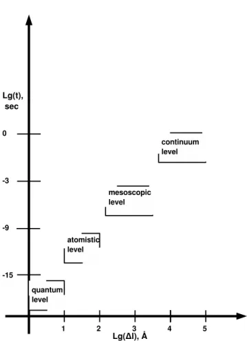
study is also a strongly innovative feature of the MDS. Here the problem that is to be solved comes to the investigation of the Hamiltonian(on a classical or on a quantum mechanic level) that one is interested in[98]; Different types of theoretical approaches are used to better understand and to predict the physical and chemical properties of the polymeric materials based on the knowledge of few input parameters[99]. The interconnection of the basic characteristics of various spatial and time scales [11], [100] should cause many complicated analytical and theoretical problems if the research scales are not to separated. Here are listed the four different levels of the polymeric system description from the molecular dynamics point of view[101]:

1. quantum level (∆l < 10˚A,∆τ < 10−15s);

2. atomistic level (∆l = 10÷ 100˚A,∆τ = 10−15÷ 10−9s);

3. mesoscale level (∆l = 100÷ 10000˚A,∆τ = 10−9÷ 10−3s);

4. continuum level (∆l > 10000˚A,∆τ > 10−3s);

where ∆l is a respective length scale and ∆τ is a characteristic relaxation time. Any level of description could be important for the simulation of the polymeric materials, depending on the task of research. Hence one has to analyze the problem thoroughly to select the most appropriate analytic tool. Let’s have a closer look at each level.

2.1.1 Quantum level

Theoretical core of a quantum level is based on Schr¨odinger equation and par-tition function. Schr¨odinger equation for a single particle in a potential:

i~∂

∂tψ(r, t) =−

~ 2m∇

2_{ψ(r, t) + U (r)ψ(r, t) (2.1)}

where i~_∂t∂ is an energy operator,∇2 _{is a Laplace operator:}

∇2_{= (} ∂ ∂x2+ ∂ ∂y2 + ∂ ∂z2) (2.2) − ~ 2m∇

2_{is a kinetic energy operator, U (r) is a time independent potential energy}

at position r of single particle, and, finally, ψ(r, t) is a probability amplitude for particle to be found at position r and at time t. Canonical partition function for canonical ensemble(thermodynamically large system in constant thermal contact with the environment, when number of constituent particles, system temperature and system volume are constant) is defined as follows:

Z =∑ s exp(−βEs) (2.3) where β = 1 kBT (2.4)

where s = 1, 2, 3, . . . are the exact microstates that system can occupy, Es is a

total energy of a system when it is in microstate s. At the quantum level, a poly-mer system is described in terms of nuclear and electronic degrees of freedom “on the go”. If we solve the Schr¨odinger equation, we obtain the wavefunction of many particles, that is the crucial function for the quantum level description. The wavefunction approaches [102] for solving the Schr¨odinger equation are very computationally demanding. This is the pay for the possibility to neglect empirical knowledge about the various effective interactions involved in the sys-tem. For example, the configuration interaction or coupled cluster methods[102], based on perturbation expansions of the many-particle wavefunction, belong to the class of wavefunction approach.

Finite temperature density functional theory methods and statistical field theory approach for quantum level of description

Another approach, the density functional theory (DFT)[103], as well, as its im-provement - the finite temperature DFT or FT DFT [104] is based on the proof of Hohenberg and Kohn [105] stating that there exists an one-to-one correspon-dence between the electron density of a system and the ground-state electronic energy. The states of the system hence are defined by an energy functional depending on the density of the particles. In contrast to the wavefunction the electron density, being the square of the wavefunction, integrated over (N− 1)-electron coordinates (where N is the total number of 1)-electrons) does not depend on N , hence it is independent of the system size. Anyway, even the most prim-itive DFT schemes are beyond any computational means on the quantum level

for the systems with number of atoms exceeding one thousand, even if we ne-glect the quantum interactions of the nuclei. For the serious analysis of the properties of polymer material this number should be increased.

The second important drawback of this approach is that the proper func-tional form relating the electron density and the ground-state energy is not known[102]. This drawback, however, can be circumvented if we use the statis-tical field theory (SFT) [106], [107], [108], [109], [110] instead of the DFT. SFT allows to reformulate the partition-function integral in a suitable functional-integral representation. This ability is obtained by linearizing the action with respect to the density field ρ(r) through introduction of a delta-functional [111] or Hubbard-Stratonovich transformation[111], that allows to replace the origi-nal particle degrees of freedom with field degrees of freedom. The resulting field function defines a set of scalar numbers to every position r in direct space, where each set represents a configuration pertaining to the field configuration space. We also have to say, that the accuracy of SFT approximations can generally be improved systematically, in contrast to FT-DFT. This can be obtained by computing higher-order corrections.

2.1.2 Atomistic level

Simulations at atomistic level have become very popular in the last 50 years [112]. At this level the electronic degrees of freedom are replaced by effective coarse-grained interactions between the nuclei. These interactions are expressed in terms of classical potentials[101]. The form of the potentials is postulated, the corresponding parameters (e.g. equilibrium bond length, force constants) are determined from quantum chemical calculations and experiments [113],[114]. The motions of the atoms are treated classically. The trajectories are propagated either deterministically or stochastically through state space, spanned by the respective particle degrees of freedom [115]. We also can say that the electronic degrees of freedom in the case of atomistic level are replaced with the force field. A force field is the total potential energy resulting from the interactions of all atoms (“explicit atom model”) or from the interactions of spherical sites comprising several atoms (“united atom model”). Usually, a force field consists of contributions from:

• bonded interactions • non-bonded interactions

Bonded interactions comprise potentials for the:

• bond length (nearest neighbor)

• the bond angle θ (second-nearest neighbor) • the torsional angle ϕ (third-nearest neighbor)

Atom pairs that form the chemical bonds can be kept at a fixed distance (r0)

by a rigid constraint using the SHAKE algorithm [116] or, alternatively, close to it by a harmonic potential

Vbond(r) =kr

2(r− r0)

where r is the distance between the bonded atoms, r0its equilibrium value, and

kris the force constant. The bond angles should be at their equilibrium values, so one of the following forms of potential can be used:

Vangle(θ) = kθ 2 (θ− θ0) 2 _(2.6) Vangle(θ) = kθ 2 (cos θ− cos θ0) 2 _(2.7) Vangle(θ) = kθ 2(1− cos(θ − θ0)) 2 _(2.8)

where θ is the bond angle, θ0 its equilibrium value, and kθ the force constant.

Equation 2.8 is for the special case θ0= 180◦. The rotations around bonds are

restricted with potentials of the shape

Vtorsion(τ ) = kτ 2 (1− cos p(τ − τ0)) 2 _(2.9) Vtorsion(τ ) = 6 ∑ m=0 Cmcosm(τ ) (2.10)

where τ is the torsional angle, τ0is its equilibrium value, kτis the force constant,

and Cm are the coefficients of a polynomial of order 6. When no rotation is

allowed around the bond, a dihedral angle can be maintained by a harmonic potential:

Vdihedral(τ ) = kτ

2 (τ− τ0)

2 _(2.11)

So, the bonded potential is the sum of all these contributions:

Vbonded(r, θ, τ ) = Vbond(r) + Vangle(θ) + Vtorsion(dihedral)(τ ) (2.12)

and it is a parametric function of the bond distances, bond angles, torsions and dihedral angles. The force constants and the equilibrium values of these variables are the parameters. All the other neighbor atoms or united atoms that are further apart the backbone of the chain are interacting via non-bonded way. The uncharged polymers they are often modeled by a Lennard-Jones potential (firstly introduced in [117]) that is very popular in the MD simulations of non-bonded interactions. It is formulated as follows:

VLJ(r) = ϵ[( σ∗ r ) 12_{− 2(}σ∗ r ) 6_{] (2.13)}

where σ is the finite distance, at which VLJ(r) is zero, ϵ is the depth of potential

well and the minimum of VLJ(r) at r = σ∗. σ∗= 2

1

6 σ. The plot of VLJ(r) versus

r is shown in the Figure 2.1. The 12-sh exponent is responsible for the

short-ranged, harsh repulsion (reflecting the reaction of the condensed matter against compression), while the 6-sh exponent is responsible for the long-ranged, much weaker attraction, holding the system together [118, 119, 120]. These repulsive and attractive interactions are illustrated in the Figure 2.2.

0.8 1 1.2 1.4 1.6 1.8 r 0 2 4 6 8 10 12 14 V (r) LJ

Fig. 2.1: The classical Lennard-Jones potential VLJ(r). For a dense liquid the principal

minimum of VLJ(r) occurs at a position close to the principal peak of g(r)

[47], see the Figure 1.2.

Fig. 2.2: Internal interactions in a polymer chain. Red arrows define the bonded

po-tential interaction, grey - the angle popo-tential interaction, green - the LJ(non-bonded) potential interaction and black - the torsion potential interaction

Monte Carlo method

The Monte Carlo methods are a class of computational algorithms that rely on repeated random sampling to compute their results. The Metropolis method is one of the oldest, most popular and simple methods of this big “family” [121]. It is a Markov chain in which a random walk is constructed in such a way that the probability of visiting a particular configurational state rN is proportional

to exp(−U (rN)

kBT ) with U (rN) being a potential energy of the configurational state rN. We should take in mind that Markov chain is a time-varying random

phenomenon for which [122]:

• the next state depends on the current state only • the number of states is finite or countable

Each Markov chain should also have a transition matrix in disposal. The tran-sition matrix is square and, if we take an element of this matrix, situated at i-th string and j-th column, we obtain the probability of direct transition from i-th state to j-th state. Sum of all the elements belonging either to the same string, or to the same column is equal to 1. A Monte Carlo move consists of two steps: 1. performing of a trial move from state i to state j according to the

corre-sponding transition matrix of the Markov chain α(i→ j)[123]

2. assessment of the probability of a trial move acc(i → j) acceptance that is calculated as

min(1, exp{−Uj−Ui

kBT })

So, the ultimate transition matrix π(i→ j) is constructed as follows:

π(i→ j) = α(i → j) × acc(i → j) (2.14) and the Metropolis scheme comprises the following steps:

1. select a particle at random and calculate its energy U (rN₎

2. give the particle a random displacement, r′ = r + ∆, and calculate its new energy U (r′_N)

3. accept the move from rN to r

′

N with probability acc(rN → r′_N) = min(1, exp{−U (r

′

N)− U(rN)

kBT }) (2.15)

The MC methods can help to cope with the problem of too long equilibration time, that no one is able to simulate. The time problem is typical for the realistic MD simulation, especially for the low temperatures and long chains. MC methodology allows to observe the huge range of ways in which MC moves may be designed to explore configuration space [124], [125]. This may help to quickly decorrelate the configurations of glassy polymer melts. The MC techniques are not efficient in the case of local MC moves (small displacement of a separate monomer [126]) because of their stochastic character, that leads to the huge increase in relaxation time [127], [128]. So, the MC moves should be nonlocal and alter large portions of a chain, changing the chain conformation at

large scales. It also should not require empty space because the melt is a dense liquid. A promising algorithm satisfying these requirements employs double-bridging moves which alter the connectivity between two neighboring chains while preserving the monodispersity of the chains [76]. The nonlocal MC moves include [129], [130], [131], [67], [68]:

1. Concerted Rotation (CONROT), that brings about a local conformational rearrangement which alters seven or eight consecutive torsion angles along a chain backbone

2. End Bridging Monte Carlo (EBMC). Here a chain end “attacks” an in-terior segment of another chain and separates it into two pieces. One of the pieces is appended to the attacking chain, while the other remains as a separate chain.

3. Double Bridging (DB) move, where two nearby segments belonging to two different chains “attack” each other and separate the chains into four pieces. The pieces are then reconnected in a different way, to create two new chains. In a system where all chains are of exactly the same length, the DB move can be designed to preserve monodispersity.

The DB move drastically changes the conformation of the two chains involved, thus relaxing the length scales on the order of the chain dimension efficiently. An inherent hazard of the algorithm is the possibility of the reverse transition of the same two chains. This drawback can be bypassed by the mixing of the local structure of the melt. It is not easy to develop an algorithm allowing to reduce the intensity of glassy slowing down of dynamics at low temperature, and, in the same time, to preserve the chain connectivity [132], [76]. However, the possible ways to solve this problem could be based on the parallel tempering [133], [134], [135], Wang-Landau sampling [125], variants thereof [136] or transition path sampling methods [137].

Explicit and united atom models. Superatoms

An explicit atom model treats one separate atom as a interaction site, while an united atom model takes some small group of atoms together into one site [113],[138],[139] such as CH or CH2. The trick is that the number of the

force centers reduces and the same computational resources allow to run the simulations at the longer time. Both explicit atom models and united atom models were widely used in the study of

1. glass-forming polymers, such as:

• polyisoprene (explicit atom model; [140], [141])

• atactic polystyrene (united atom model; [142],[143],[144], [145],[146]) • bisphenol-A polycarbonate (united atom model;[145],[146])

• cis-trans 1,4-polybutadiene (united and explicit atom models; [113],[147],

[148],[114],[149],[150],[151], [152],[153],[154])

• 1,2-polybutadiene(explicit atom model; [155]) • polyvinyl(methylether)[156]

• polyethylene(altpropylene) [157]

2. binary polymer mixtures (united atom model; [158]) 3. polyethylene oxide (explicit atom models; [159] )

The most important advantage of these types of modeling is the possibility of consequent comparison of the simulation results with experiments. But this comparison requires, however, a very high level of attention to both structural and dynamic properties because we still can not guarantee the accurate predic-tion of the dynamics even if we have the same structural properties for both simulation and experimental research[113]. The same conclusion can also be made for non-polymeric amorphous SiO2 [98],[160]. This suggests that the

design of a chemically realistic model, aiming at a parameter-free compari-son between simulation and experiment, should involve information about both structural and dynamic properties. When we know the force-fields we may ap-ply a huge range of particle-based computer simulation techniques to simulate the statistical behavior of the particle system under various external conditions [161],[124],[162],[112]. For instance, a molecular dynamics simulation is con-ducted by numerically integrating in time t Hamilton’s equations of motion,

dpi dt =− ∂H(r, p) ∂ri , dri dt =− ∂H(r, p) ∂pi , (2.16) where H(r, p) is a Hamiltonian: H(r, p) = N ∑ i=1 p2 i 2mi + Φ(r), (2.17)

with the variables r = (r1, . . . , rN) and p = (p1, . . . , pN) denoting the sets of

atomic positions and momenta, while mi is the mass of the i-th atom [112].

∑N i=1

p2_i

2mi represent kinetic and Φ(r) - potential energy of a system consisting of N particles. In the absence of any external field, Φ(r) can be written as

Φ(r)≈ N ∑ i N ∑ j>i Φef f_ij (rij) (2.18) where rij =|ri− rj| (2.19)

is the distance between particle i and j . The sum over atomic pairs can comprise effective interactions between bonded and non-bonded atoms. A commonly used two-parameter potential model for describing non-bonded interactions between a pair of neutral atoms is the Lennard-Jones 6− 12 potential (see the formula 2.13 on page 24).The formulas 2.13,2.16,2.17,2.18,2.19 represent a set of 6N -first-order differential equations. These equations are integrated numerically with the help of the initial set of particle positions and momenta as well as periodic boundary conditions[163] in order to reduce the influence of the finite size effects.

The periodic boundary conditions are applied as follows: the cubic box represented the given system is replicated throughout space to form an infinite

lattice. During the simulation, as a molecule moves in the original box, its periodic image in each of the neighboring boxes moves in the same way. Thus, as a molecule leaves the central box, one of its images will enter through the opposite face.

The resulting trajectory of the solution of the set of equations must be representative and evolve a sufficiently long time in state space, to fulfill the quasi-ergodic theorem, expressed by [164]

ϑobs=⟨ϑens⟩ = lim

trun→∞

ϑt_run, (2.20)

where ϑobs is the macroscopic physical quantity and ϑens is the

correspond-ing ensemble average, while ϑtrun is the time-average of the ϑobs over sim-ulation time trun. The simulations at atomistic level provided physical

in-sights into the equilibrium properties of many other physical systems, like e.g. membranes [165, 166, 167, 168, 169, 170, 171, 172, 173, 174], proteins [175, 176, 177, 173, 178, 179], ABA triblock copolymers (the polymers made of two or more chemically distinct sequences of monomer units that are covalently linked together) [180], polyelectrolytes [181],[182],[183], [184], [185],[186], [187], etc. Simulations at the atomistic level allow us to investigate the thermophysi-cal and rheologithermophysi-cal properties of specific polymers, including their glassy state. But up to now the widespread use of the simulations at the atomistic level is severely constrained by the limits of modern computational power. For example, in [101] the atomistic simulation (by the means of the latest MD techniques[124] ) of the liquid consisting of 106 identical argon atoms interacting pairwise via the LJ potential (see 2.13) for up to 106 time steps would represent only 10 ns of real time because of the extremely small time scale of LJ potential[106]. This system is 2-dimensional and is supposed(with significant simplifications) to simulate the phase-separated poly- (styrene-butadiene-styrene) SBS triblock copolymer system [188]. In turn, the equilibration time of the polymer is about 10−3 s [106] and may increase in the vicinity of a glass transition and with longer chain lengths. The relaxation times in entangled polymer melts grow faster than the third power of the molecular weight [70]. So, one need at least 105 _{more computational power to equilibrate this simplified 2-dimensional}

sys-tem with the means of state-of-the-art MD simulation. The same conclusions about impossibility of atomistic simulation of the real relaxation processes are made in [69],[67],[76]. Another task is to truncate the long-range interactions in the system of interest in order to get rid of the enormous number of pairwise in-teractions. Most of these interactions take place at extremely long distances, so we can apply the truncation condition if we do are not interested in analysis of the long-range interactions. Usually, this truncation is applied in the following way(the generalized truncated LJ potential [69]):

VLJ(p, q; r) = { _ϵ q−p[p( σ∗ r) q_{− q(}σ∗ r) p_{] + V} cut if r≤ rcut 0 otherwise (2.21)

where the value of the constant Vcut is chosen to ensure VLJ(p, q; rcut) = 0 at r = rcut = 2.5 σ. This shift is set to eliminate the discontinuity and reduce relative calculus artifacts. The minimum of the potential V (p, q; r) is at r = σ∗, with a constant depth VLJ(p, q; r = σ∗) = −ϵ. Position of the minimum

re-mains constant when p and q parameters are changed. Note that upon choosing (p, q) = (6, 12) the classical Lennard-Jones potential is recovered.

Finite temperature density functional theory methods and statistical field theory approach for atomistic level of description

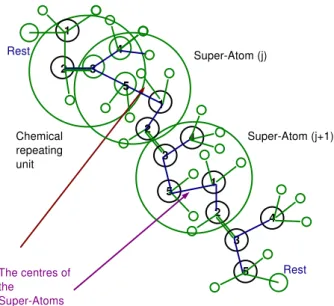
FT-DFT methods [103], or SFT approach [189],[190](both already mentioned in the quantum level simulations) are used at the atomic level of description to avoid the summation over atomic pairs. The FT-DFT and SFT methodolo-gies allow to handle a fewer number of degrees of freedom with respect to the particle-based approach. SFT methods also overcome the problem of long equi-libration times typical for the particle-based approaches by reformulating the particle systems in functional integral formulation and throwing away configura-tions of low statistical weight. Last feature becomes possible with use of effective calculation strategies. One more advantage of the SFT methods compared to the particle-based simulation techniques is an absence of the particle insertion moves, that drastically decrease efficiency of the the grand canonical simulations of open polymer systems at low temperatures [190], [191]. The temperature of the open systems in the range of physical interest causes an increase of inter-action strength between the monomers, so the particle insertion becomes more problematic. Another serious problem of the atomistic particle-based simula-tions is the sophisticated nature of any polymer. It becomes especially evident at the higher levels of coarse-graining. So, if we take the united atom unit, or even a larger entity - a superatom unit (order of 10 non-hydrogen atoms or approximately one chemical unit, such as, e.g. a styrene unit in polystyrene, an amino acid in a protein, four methylene groups in polyethylene, etc. [139], for a graphic representation please see the Figure 2.3 [192]), and try to parameterize the effective interactions between that single unit and other units like that, we meet serious problems. Each such a unit consists of subchains. This subchain can adopt very many different conformations. Baschnagel et.al. [138] offered a complicated procedure, having at the first step the fully atomistic simulations of the united atoms and, then, computing the spatial correlation functions among the center-of-mass positions of the subchains. These correlation functions can in turn be used to build models for two-, three-, four- and higher inter-particle potential functions. The inter-particle effective potential functions could subse-quently be employed for particle-based simulations of larger systems.

Different tricks allowing to reduce the simulation time of MD simulations. Method of Li and Chou. TDGL

The slowness of the traditional MD methods forced the scientists to find an-other simulation methodologies. For example, the modeling of the carbon nan-otubes(CNT)( the allotropes of carbon with a cylindrical nanostructure having the remarkably high stiffness at low density [194, 195]) in the atomistic scale evidenced a very high level of time consuming (see e.g. [196]), so a new molec-ular structural mechanics method has been developed by Li and Chou [197]. In this method, a single-walled carbon nanotube is viewed as a space frame, where the covalent bonds are represented as connecting beams and the carbon atoms as joint nodes. So, if one exploits the molecular structural mechanics, he can determine the elastic constants of the equivalent beam including ten-sile resistance, flexural rigidity, and torsional stiffness. This feature is based on equivalence between local potential energies in computational chemistry and el-emental strain energies in structural mechanics [198]. The molecular structural

Fig. 2.3: Coarse-graining of polyisoprene. The superatoms are centered in the middle

of the bond linking two chemical repeat units (rather than at the center of a chemical repeat unit), in order to represent more realistically the excluded volume envelope of the molecule [193]

mechanics method was also used for the viscoelastic matrix of CNT/polymer composite(where the small sections of CNT are used as a reinforcing phase in order to improve the elastic properties of a polymer matrix, see [199], [200], [201]) in [202]. The time-dependent Ginzburg-Landau method (TDGL) is an atomistic method for simulating the structural evolution of phase-separation in polymer blends and block copolymers [203]. It is based on the Cahn-Hilliard-Cook (CHC) nonlinear diffusion equation for a binary blend [204], [205], [206]. In the TDGL method, a free-energy function is minimized to simulate a temper-ature quench from the miscible region of the phase diagram to the immiscible region. Thus, the resulting time-dependent structural evolution of the polymer blend can be investigated by solving the TDGL/CHC equation for the time dependence of the local blend concentration. TDGL was simplified by Oono et. al. [207], [208] in cell dynamic method (CDM) that was derived from the discretized TDGL equation. The TDGL and CDM methods have been used to investigate the phase-separation of:

• polymer nanocomposites [209], [210]

• polymer blends in the presence of nanoparticles [211]; particle-field

poly-mer systems [212]

Brownian dynamics

Finally, we have to introduce the Brownian dynamics (BD) method that is often used in the case of polymer solutions study [216], [217], [218]. The BD simulation introduces several new approximations allowing to perform simulations on the larger timescale (microseconds instead of nanoseconds), if compared to MD. The basic equation of the BD is the following one (known as Langevin equation):

∑

j̸=i

FijC− γpi+ σζi(t) = mi d2−→ri

dt2 (2.22)

with F_ijC being the conservative force of particle j acting on particle i, γ and σ are constants depending on the system, pi is the momentum of particle i, ζ(t)

is a Gaussian random noise term, mi is the atomic mass and −→ri is the atomic

position. Let us try to list the main differences between BD and MD:

• in BD the explicit description of solvent molecules used in MD is replaced

with an implicit continuum solvent description

• the internal motions of molecules are typically ignored, so on can employ

a much larger timestep than that of MD

Hence, BD is particularly useful for multicomponent systems where there is a large gap of time scale governing the motion of different components, for example, in polymersolvent mixture, where a short timestep is needed to resolve the fast motion of the solvent molecules, whereas the evolution of the slower modes of the system requires a larger timestep. So, the dissipative (−γp) and random (σζ(t)) force terms represent the effect of the solvent molecules on the system. The effect of the fluctuating forces term is that the energy and momentum are no longer conserved. The macroscopic behavior of the system is no more hydrodynamic compared to MD. In addition, the effect of one solute molecule on another through the flow of solvent molecules is neglected. Thus, BD can only reproduce the diffusion properties but not the hydrodynamic flow properties.

2.1.3 Mesoscale level

The mesoscale level of description is the intermediate level between the atomistic and continuum scale. It ignores the atomic details below a threshold of about 1 nm. The mesoscale level, however, preserves the generic features of a polymer, such as connectivity, space-filling characteristics and architecture [138], [219]. The evolution from more detailed to more coarse-grained levels of description of modeling of polymers is shown at Figure 2.4 [69].

Lattice models

Various generic models have been studied for glass-forming polymers so far. These models can be divided onto 2 large subclasses:

• lattice models