This thesis is composed by three experiments that explore the role of information in individual decision-making.
In Chapter 1 it is presented an experimental test of the contextual inference theory (Kamenica,2008). The experiment shows that the dimension of choice sets conveys payoff-relevant information in decision-making: even when options are not directly observable, the likelihood of finding an option that fits individual tastes can be inferred from the set size.
Information on the lenght of a product line is then shown to be relevant in individual decision making.
In Chapter 2 the decision-maker is presented with payoff irrelevant information: group-membership and others' behavior. The experiment test if and how these information affect individual decision of behaving ethically. The results provide evidence of the effectiveness of these information in shaping moral behavior.
Chapter 3 aims at going into the black box of information processing under uncertainty with an
eye-tracking experiment. The aim of this last chapter is to contribute to the understanding of the choice process under different dimensions of the choice sets (small and large), and its relation with the response time.
I would like to thank Giuseppe Ciccarone for supervision and support; the staff of the laboratories where I run these experiments: EXE-LAB at Sapienza, CESARE Lab at Luiss, and WiSo Lab at the University of Hamburg; the Department of Economics and Law at Sapienza for financial support.
Irene Maria Buso ∗
This version: February, 2017
Abstract
The paradoxical finding of the preference for small sets of products (Iyengar and Lepper, 2000) has been explained with cognitive costs and regret. Instead, Kamenica (2008) suggests that the set size conveys a payoff relevant information: in small set there are the most popular product. The present experimental analysis aims to test if the contextual inference theory can explain the increased willingness to take a product from small sets. The design rules out alternative explanations, and find a support for the contextual inference hypothesis: the information about the set size conveys payoff relevant information in favor of small sets; however, the information seems not be about the popularity of the option according to the beliefs analysis.
∗
Buso: University of Rome ”La Sapienza”, Department of Economics and Law, Rome, Italy.
1
Introduction
The paradoxical finding that having extensive choice sets may have detrimental consequences for consumer welfare (Iyengar and Lepper, 2000) has opened a new strand of literature that aims at identifying the antecedences and consequences of large sets in decision making. The failure of some papers to replicate these paradoxical findings (Chernev (2003);Scheibehenne et al. (2009)), stresses the necessity to identify the circumstances that lead to the arise of this phenomenon. The cognitive overload that the processing of many options implies has been proposed as a possible explanation for this phenomenon, that is consequently often labelled as choice overload. Reutskaja and Hogarth (2009) show experimental evidence in favor of the moderating role that cognitive costs play in decreased satisfaction in small sets. Also, the emotional aspects of choices as regrets have been proposed as a moderator of the phenomenon (e.g. Sarver (2008)). An alternative explanation based on standard assumption of utility maximizing consumers has been suggested by Kamenica (2008): the dimension of the choice set (large vs small) conveys payoff-relevant information on the products. This model explains the preference for small sets assuming asymmetric information between firms and consumers on the distribution of tastes in the population and a fraction of consumer uninformed on their tastes. The uninformed consumers look for the most popular options since these are more likely to suit them. They can infer information on the popularity of the products from the length of the product line: the average popularity of the products in the small set is higher than in the large set. It follows that they are more willing to pick at random a product from a small set than from a large set because it is more likely that they pick a product that satisfies them. The present experimental analysis aims at testing if contextual inference can to some extent explain the preference for small sets. The design relies on the standard framework used to test willingness to purchase a product in large and small sets: a between-subjects study where the experimental groups are alternatively presented with a small or large set of products and have to decide to take a fixed monetary fee or a product from the set. This baseline design is modified implementing the assumption on consumers’ information: uncertainty about preferences is introduced offering products that subjects cannot see, so that they do not know their subjective values. The only information given is on the dimension of the choice set. This design allows to rule out preference for small sets due to cognitive costs since participants do not have differential amounts of information to process in the small and large sets. They know that the offers in the sets is the real product line offered by a store in Rome. They can then rely on the length of the product line to infer the popularity. If they choose to take a product instead of money, it is randomly drawn from the set. The choice task is done on three products:
chocolate, yogurts and crisps.To preempt the results, in two of the three procuct categories the proportion of people that prefer to take whatever product from the small set is higher than from the large one. This evidence supports the contextual inference as an explanation of the preference for small sets, and this evidence cannot be explained by cognitive costs and regret since they are eliminated by the design itself. In section 2, the literature literature on preference for small set is reviewed and the reserch questions are introduced. In section 3 the experimental design is presented together with the hypotheses tested. In Section 4, the experimental procedure is presented in details. Results are reported in section 5, and section 6 concludes.
2
Literature Review and Reserch Questions
The experimental analysis of Iyengar and Lepper (2000) has highlighted the negative effect that an increasing number of options may have on consumer satisfaction and willingness to purchase a product. This phenomenon is a paradox in choice theory, since enlarging the choice set should not worsen consumers’ welfare. These detrimental consequences have being explained in terms of cost-benefits analysis, where an increasing number of options raises both the opportunities of consumption and the costs of choices in terms of cognitive effort (e.g. Roberts and Lattin (1991); Reutskaja and Hogarth (2009)) and time (Botti and Hsee, 2010) rise. Regret has been shown to be a consequence of the increasing number of choices (e.g.Iyengar and Lepper (2000) ; Inbar et al. (2011)); As a consequence, an anticipatory regret could be an antecedent of choice overload (e.g. Sarver (2008)). Also, individual attitudes toward maximizing and satisficing (e.g. Schwartz (2004)) have been shown to have a role in satisfaction from different sized sets. Chernev et al. (2015) identifies the most relevant moderating factors of choice overload in a meta-analysis: decision task difficulty, choice set complexity, preference uncertainty, and effort-minimizing goal. Kamenica (2008) suggests that the preference for small choice sets may be due not to cognitive limitations or emotional factors, but to the rational inference of the consumers. When there is preference uncertainty and asymmetric information between consumers and firms on the distribution of tastes, the uninformed consumer infers the popularity of the options from the set size; this hypothesis relies on previous literature showing that the consumer may be uncertain on the subjetive value of the options. Instead, the consumer has less uncertainty on how his/her tastes compare with the tastes of the rest of the population. Hence, individual preferences are defined not absolutely, but relatively to others’ preferences (Wernerfelt, 1995). According to this argument, the popularity of a product becomes a way to establish which option is more likely to fit the tastes of the consumer
who is uncertain about his/her preferences (if one believes that his/her tastes are not different from the average of the population, that is, not atypical). Prelec et al. (1997) show that this kind of preference uncertainty implies that consumption choices are sensitive to the context, since different contexts may imply different inferences about other tastes. This argument is used by Kamenica (2008) in order to explain the choice overload phenomenon: the context (that is, small or large set) affects the inference on the popularity of the options available; in particular, small choice sets provide better information on the popularity of the options inside, and here arises the preference for choosing from small sets. Indeed, on the supply side, the model assumes that firms know the distribution of tastes in the population, and they build the product line according to these tastes in order to maximize their profit: they want to offer the most popular products; however, the average popularity of the products offered is decreasing in the breath of the product line: the first product introduced is the most popular, the second is the second most popular, an so on. Hence, products with lower popularity are sequencially introduced, and the larger the product line the more products are introduced with relatively lower popularity.1 From the demand side, the model assumes that there is a fraction of consumers that is uninformed about its tastes and about the distribution of tastes in the population. Since there is asymmetric information between consumers and firms, and it is assumed that consumers know this asymmetry, the uninformed consumer can infer the distribution of tastes from the production choices of the firms. In particular, they can infer the average popularity of the products from the number of products offered: since they cannot do better than choose randomly2, they are more willing to pick whatever product when the product line is limited than when it is large. Indeed, they have more chances to take a product that is likely to suit them from a small set. Therefore, the model predicts the preference for small sets as an inference of payoff-relevant information from the set size. Under the preference uncertainty and information asymmetry, it is payoff maximizing choosing from the small set even in absence of cognitve limitations and emotional factors in decision-making. Hence, the following desing aim to test experimentally if the preference for taking products from small sets can be explained by the inference-based mechanism proposed by the model of Kamenica (2008).
1It has to be noticed that the small sets contains the most popular options because this behaviour is profit
maxi-mizing for the firms. If the small sets were a random selection from a larger sets, the small sets would not have this property. For example, in Reutskaja and Nagel (2011), the small sets are chosen randomlt from the small sets. It follows that the large sets contains a greater amount of (approximately similar) good options than small sets, and this increases th efficiency of choice from large sets.
3
Experimental Design and Hypotheses Testing
The present experiment relies on the standard framework in experiments on over-choices: it is a between-subjects experiment where the willingness to purchase a product rather than accept a fixed monetary payment is compared in the two experimental conditions, that is when an extensive or a small choice set are provided to the participants. The new element with respect to previous studies on this topic is that the participants do not see the options in the set: the items are presented inside bags . The subjects choose to take one product at random from the set or a the monetary fee. Hence, the partcipants are put on the same condition of preference uncertainty assumed by the contextual-inference theory, since no one has the possibility to observe the products and evaluate their subjective values, and they are forced to choose at random in case they decide to pick one product from the set; this condition (preference uncertainty) should imply the necessity to infer the popularity of the products, since they cannot do best than choose at random from the choice set. They were told that in case they chose to take a product, they would receive one of the products of the set randomly drawn; it was explicitly stated that they would be allowed to see only the drawn product, and not the whole content of the set. Instead, if they took the monetary payment, the would receive an amount of money equal to the average value of the products in the set. Since it is not possibile to see the products in the set before the choices, cognitive costs cannot account for a preference for the small set in this design. Further, since the whole product line cannot be seen after the choices, anticipated regret cannot explain the preference for taking a product from the small set as well.
Another elements of the design that is fundamental to test contextual inference theory is that the participants know that the products offered are the entire product line of a store: they know that the options within a set are of the same brand and they are the actual and whole assortment of that product offered by a store in Rome. The name of the brand and of the store was not told to them. Since the product offered are a real assortment offered by a supplier, they may consider the assortment as informative on population tastes. For this reason real products have been used, instead of abstract induced value objects3. The two experimental conditions, small and large sets,
are implemented as follow: to the group of subjects in the small set condition, the number of items offered is taken from a store with a limited product line; to the group of subjects in the large set
3
since these products do not have an induced-value, individual homegrown preferences are taken into account asking for a non-incentivized liking-rating score from 0 to 10 and frequency of consumption.
Note that the theory may be tested with value induced objects creating experimentally the supply side of the market and inducing preference over objects with an asymmetry of information. However, using real products the inference process may be elicited more unconsiuosly. Further,is the standard way in which choice overload has been studied.Therefore, keeping this framework is more helpful for a comparison with previous findings.
condition, the offer is taken from stores with a large product line. In each session the choice is done for three products: chocolate, yoghurts and chips.
The prediction of the theory is that uninformed subjects prefer to take whatever product from the small set than whatever product from the large set because the context (small vs large set) conveys the information about the likelihood of receiving a product that suits their preference: the smaller is the product line the more it is probable to take a product that they may like. Hence, the present experiment tests the following hypothesis:
Hypothesis 1: The probability of taking a product in small sets is graeter than in large sets.
According to this hypothesis, subjects should choose to take a product rather than money from the small sets more ofter in the large sets. Preference for small sets in such an experimental setting cannot be explained by cognitive costs since the costs of processing information are eliminated not allowing to see and compare the products and choose among them. Neither by regret, because the product line offered is not observable after the choice. Instead, in line with the contextual inference argument, the participants may expect that more popular products are in the small sets (for exam-ple, traditional flavors of chocolate: dark, milk..), since the shops offering few flavors select the most standard (usually liked) ones; instead, in the large set they may pick an unsual product that is less likely to suit their tastes,as spiced chocolate. To add further evidence to the contextual inference theory, the partcipants’ beliefs on the popularity of the products in the sets are elicited. Through a survey before the experiment, there were collecte the liking-ratings over the products offered in the experiment by a sample of 15 potencial consumers. Products were rated them from 0 to 10, and the partcipants were incetivized knowing that would have received one of the products that they rated at least 7. The subjects in the experiment knew this information, and they have to guess how many products in the offered set recevived an average rating equal to 7 or higher. According to the contextual inference theory, one should choose more likely to take a product if he/she believes that there is a higher percentage of high rated, that is popular, products. Furthermore, extending the argument of Kamenica (2008), one may prefer the small set if he/ she believes that in the large set there is a higher proportion of niche products that are then unlikely to suit the tastes of the average consumer. The guessing on the number of products that received a rating equal or lower than 4 is then introduced. From the third class session also the guessing on the number of products that re-ceived a rating equal or lower than 4 is introduced. Further, The following hypotheses are then tested:
Hypothesis 2a: The choice of acceptance is positively associated with the beliefs of a greater proportion of high-rate products and negatively associated with the beliefs of a lower proportion of low-rated products is the choice set.
Hypothesis 2b: In small sets it is expected to be a greater proportion of high-rated products and a lower proportion of low rated products
4
Experimental Protocol
The experimental sessions were run in May and June 2017 at the University of Rome ”La Sapienza”, in the faculty of economics. They were five in total. The first three sessions were run in classes and the other two sessions in the EXE LAB, the experimental laboratory of the faculty.4
Class Sessions In the first session (the 18th of May) 22 subjects were assigned to the small set condition and 18 to the large set one. In the second session (the 25th of May) 31 subjects were assigned to the small set condition and 31 to the large set one. In the third session (the 26th of May) 18 subjects were assigned to the small set condition and 16 to the large set one. The products used in the first session were chocolate and yogurt; in the second and third sessions the products were chocolate, yogurt and crisps. In the small set condition the subjects chose among 6 types of chocolate and 8 yogurts, and 5 types of crisps. In the large set condition they choose among 25 chocolates and 30 yogurts and 27 crisps. Beliefs on each of these products were elicited only on the number of products rated higher than 7. All sessions were run with pencil and paper and subjects in the different experimental conditions were possibily not sitting near to each other. The participants were bachelor students. The tasks were six in total (three choice tasks and three belief tasks) and one was randomly chosen for payment. In the case one of the choice tasks was chosen for payment, the students would have received the product or the monetary payment, according to their choices; the monetary payment was 2 euros for chocolate and crisps and 1.5 euros for the yogurt, but they were not explicitly told the amount of the payment they would have received during the session. They just knew that the fixed moentary payment was equal to the average value of the products in
the set. In the case one belief tasks was chosen for payment, they would have received 5 euros if the guessing was correct , and 5 minus the quadratic error if not correct without the possibility of negative payoffs. The experiment lasted 20 minutes; the instructions were read aloud sequencially: the participants were instructed to complete each task of the experiment after it was read aloud by the experimenter, and they were not allowed to look at the following tasks before being authorized, that is before the tasks were read aloud. No show-up fee was provided for these class sessions, and one third of the subjects was randomly chosen for payment, except for the last class session where they were all paid. In the first two sessions, a belief task was drawn for payment in front of the class and the students received the payment at the beginning of the following lesson. The average payment was 2 euros. In the last session the crisps choice task was drawn for payment; the subject received the products after few days.
Laboratory Sessions Two laboratory sessions were run on the 15th of June with 60 students. The sessions were computerized and programed in ztree (Fischbacher, 2007). The participants were recruited by the didactic manager who sent an email to the institutional email address of all the students of the faculty of economics, and they registered replying to it. They received a show-up fee of 5 euros. The large set treatment was run in the first session, and small set treatment in the second one with 30 participants in each. Control variables about sex, age and education (university year) were collected. In the small set condition they chose among 6 types of chocolate, 8 yogurts and 5 crisps. In the large set condition they chose among 38 types of chocolate, 30 yogurts and 22 crisps. Beliefs about the number of products rated 7 or more and 4 or less were elicited. In the case one of the belief sessions was drawn for payment, they were paid for one of the two beliefs chosen randomly. Differently from the class sessions, the amount of the fixed monetary payment that partcipants would have received in the case they did not choose a product was explicitly declared in the instructions. The payment rule for guessing tasks was different from the class sessions: 5 euros for the correct guessing, and 5 minus the error in case of incorrect guessing. The experiment lasted 30 minutes and payment was administered individually after each session. The instructions were on the screen and they were read aloud at the beginning of each of the six tasks of the experiment. They knew that in case one of the tasks with products was chosen estraction with replacement was possible: the set contained the same products for all the subjects. The products were physically in the laboratory when the sessions were run: products were inside bags so that they could not be seen. One subject was recruited at the beginning of each session among the participants to look inside these bags and guarantee the other participants that there really was the variety of different
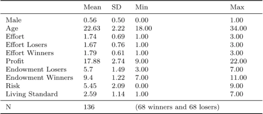
Table 1: Summary Statistics on Class Sessions
Rating is a variable that assumes integer values from 0 to 10 and it is the self-reported liking of each product. Frequency takes values from 1 (every day) to 5 (never), and represents the frequency of consumption of the product.
.
Mean SD Min Max
Rating Chocolate 7.5 1.7 3 10 Rating Yoghurt 5.5 2.3 0 10 Rating Crips 7.4 2 0 10 Frequency Chocolate 2.1 0.9 1 5 Frequency Yoghurt 2.7 1.14 1 5 Frequency Crisps 2.7 0.8 2 5
N 135 (Chocolate and Yoghurt) 95 (Chips)
Table 2: Summary Statistics on Laboratory Sessions
Mean SD Min Max Rating Chocolate 7.75 1.5 3 10 Rating Yoghurt 6.3 2.1 0 10 Rating Crisps 6.7 2.4 0 10 Frequency Chocolate 2 0.85 1 4 Frequency Yoghurt 2.5 1.1 0 5 Frequency Crisps 2.8 1 1 5 N 59
products declared; this subject did not complete the tasks and received a fixed payment equal to 7 euros. One of the six tasks was randomly chosen for payment. In the first session the product task with crisps was paid giving the show-up fee plus 2 euros to those who did not choose the product and one random product to the others5. In the second session the belief task with chocolate was paid and the average payment was approximately 8 euros including the show-up fee.
5
Results
The summary statistics of the data from class sessions and laboratory sessions are reported in table 1 and 2. A summary of the finding of this section is in table 3.
The results of the regression analyses on Class session data (5.1) and laboratory session data (5.2) are first presented separately. Then, the data are analyzed pooled (5.3). Finally, the beliefs analysis is presented.
Table 3: Summary of the Findings
This table shows the percetages of accpected products in small (% products Small Set ) and large sets (% products Large Set ). N obs is the number of observations. P-Value is the significance level of the set size in the regression analyses below.
.
% Products Small Set %Products Large Set N obs P-value Class Chocolate 36% 17% 135 0.07
Class Yoghurt 15% 15% 135 not significant
Class Crips 48% 30% 94 0.04
All Class Products 30% 19% 364 0.01
Laboratory Chocolate 29% 21% 59 not significant Laboratory Yoghurt 20% 15% 59 not significant Laboratory Crisps 33% 33% 59 0.06
All Laboratory Products 27% 24% 177 0.03 All Session Products 29% 21% 541 0.006
5.1 Class Sessions
Firts, the data from class session are analyzed product by product type through logistic regressions. Then, all data from class sessions are analyzed using a mixed-effects logistic regression with random intercept that account for the repeated measurement. The results of the regression analyses are reported in table 4.
Chocolate Class The dimension of the set significantly (p-value=0.07) affects the decision to take the chocolate or not: the predicted probability of taking chocolate is 15% in the large set and 29% in the small set.
Yoghurt Class The decision whether to take the yogurt or not was not significantly affected nei-ther by the set size nor by onei-ther covariates.
Crisps Class The dimension of the set significantly (p-value=0.04) affects the decision to take the crisps or not: the predicted probability of taking crisps is 25% in the large set and 48% in the small set.
Table 4: Regression Analysis on Class Sessions’ data
This table displays the results of the logistic regression analysis on data from class sessions. Regressions 1, 2 and 3 are run for single products. Regression 4 is run on all class data using a mixed-effects logit with random intercept. The values in the table are the Odds Ratios.
The dependent variable of the regression is Acceptance: a dummy variable equal to 1 when the product is accepted and equal to 0 when the product is not accepted.
Treatment is a dummy variable equal to 1 in the small set condition and equal to 0 in the large set condition. Guessing 7 is the proportion of products that, according to their guessings, received a rating equal or higher than 7.
.
(1) (2) (3) (4)
Acceptance Chocolate Acceptance Yoghurt Acceptance Crisps Acceptance All Class Sessions
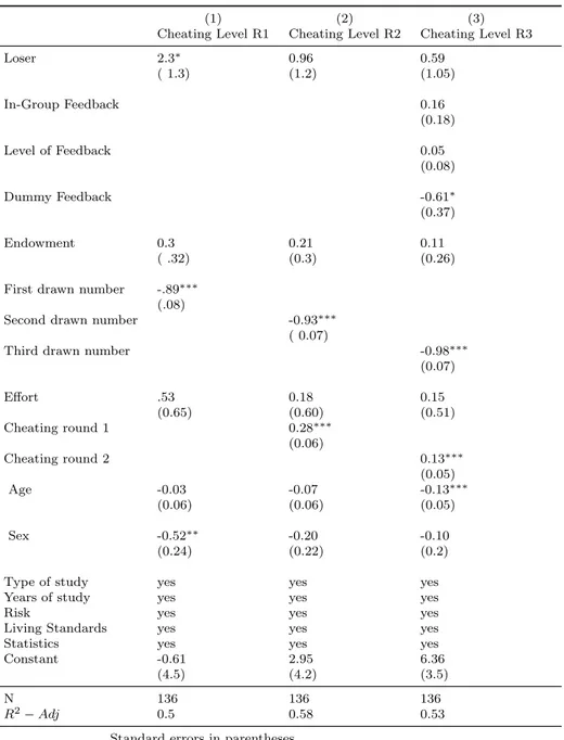
Treatment 2.2∗ 1.15 2.59∗∗ 0.671∗∗ (0.95) (0.57) (1.22) (0.262) Rating 1.45∗∗ 1.17 1.17 0.258∗∗∗ (0.25) (0.19) (0.2) (0.0932) Frequency 0.74 0.73 0.38∗∗∗ -0.396∗∗ (0.21) (0.22) (0.14) (0.184) Guessing 7 0.55 0.66 0.95 -0.181 (0.56) (0.76) (1.03) (0.607) Constant 0.03∗∗ 2.95 0.17 -2.231∗∗ (0.05) (0.3) (2.95) (1.044) N 135 135 94 364 (number of groups: 3) P (LRchi2) 0.001 0.18 0.001 0.0001
Standard errors in parentheses *** p<0.01, ** p<0.05, * p<0.1
All Class Sessions Considering the data in all class session, the dimension of the set significantly (p-value=0.011) affects the decision to take one of the products from the set. Also, Rating and Fre-quency positively affect the choice to take the product. The predicted probability of taking crisps is 16% in the large set and 28% in the small set.
5.2 Lab Sessions
Firts, the data from laboratory sessions are analyzed product by product type through logistic re-gressions. Then, all data from lab sessions are analyzed using a mixed-effects logistic regression with random intercept that account for the repeated measurement. The results of the regression analyses are reported in table 5.
Note that the significance of the set dimension is lower in the lab sessions than in the class ones. This may be because the subjects in the laboratory were explicitly told the amount of the mone-tary payment in case they did not choose the product. This may have decreased the difference in the acceptance rate in the two sets since the average value of the set was homogenized across the experimental conditions. This evidence is in line with previous findings on the moderating role of an ideal point in choice overload phenomenon (Chernev, 2003).
Chocolate Laboratory None of the covariates significantly affect the decision of taking the choco-late or not. Even if the treatment variable does not reach the significance level, the results slightly go in the predicted direction: in the large set condition 23 persons chose money and 6 chose chocolate. In the small set condition 21 persons chose money and 9 chocolate.
Yoghurt Laboratory None of the covariates significantly affect the decision of taking the product or not, except for the guessing on the number of products that were rated equal or lower than 4. Even if the treatment variable does not reach the statistical significance, the results slightly go in the predicted direction: in the large set condition 24 persons chose money and 5 yoghurt. In the small set condition 24 persons chose money and 6 yoghurt.
Crisps Laboratory The dimension of the set significantly (p-value=0.06) affects the decision to take crisps or not: the predicted probability of taking crisps is 4% in the large set and 30% in the small one. The evaluation of the crisps significantly (p-value=0.01) increases the willingness to take them as well as the beliefs about the number of high rated crisps (p-value=0.09).
Table 5: Regression Analysis on Laboratory Sessions’ data
This table shows the results of the logistic regression on data from class sessions.Regressions 1, 2 and 3 are run for single products. Regression 4 is run on all class data using a mixed-effects logit with random intercept. The values in the table are the Odds Ratios. Treatment is a dummy variable equal to 1 in the small set condition and 0 in the large set one. The dependent variable of the regression is Acceptance: a dummy variable equal to 1 when the product is accepted and equal to 0 when the product is not accepted.
Guessing 7 and 4 is the proportion of products that, according to the guessing, received a rating equal or higher than 7 and equal or lower than 4 respectively. Education ranges from 1 to 6: it is equal to 1 at the first year of the bachelor, 5 at the last year of the master, otherwise 6.
.
(1) (2) (3) (4)
Acceptance Chocolate Acceptance Yoghurt Acceptance Chips Acceptance All Lab Products
Treatment 1.8 2.4 8.8∗ 0.945∗∗ (1.35) (2.12) (10.3) (0.457) Rating 2.02 2.5 3.38∗∗∗ 0.827∗∗∗ (0.73) (0.92) (1.6) (0.179) Frequency 1.18 1.6 0.05 0.158 (0.68) (0.83) (0.25) (0.281) Guessing 7 42.7 0.05 0.006∗ -0.257 (109) (0.15) (0.37) (1.277) Guessing 4 6.63 0.001∗∗ 0.12 -2.414∗ (15.6) (0.005) (0.4) (1.394) Education 1.35 1.2 1.5 0.194 (0.41) (0.38) (0.51) (0.163) Male 0.62 2 4.8 0.307 (0.45) (1.9) (4.8) (0.426) Age -0.04 0.93 1.1 -0.125 (0.02) (0.21) (0.32) (0.112) Constant 0.81 0.002 0.0001 -5.532∗∗ (4.7) ( 0.01) (0.0002) (2.695) N 59 59 59 177 (n. of groups 3) P (LRchi2) 0.06 0.04 0.0001 0.0006
Standard errors in parentheses *** p<0.01, ** p<0.05, * p<0.1
All Lab Sessions Pooling all laboratory data, the dimension of the set significantly (p-value=0.03) affects the decision to take a product or not: the predicted probability of taking a product is 10% in the large set and 23% in the small one. The evaluation of the products significantly (p-value=0.001) increases the willingness to take them; further, the beliefs about the number of low rated products has a negative relation with the decision of acceptance (p-value=0.08).
Table 6: Regression Analysis on All Sessions’ data
This table shows the results of the logistic regression on data from all sessions. The values in the table are the Odds Ratios. Regressions 1, 2 and 3 are run for single products. Regression 4 is run on all class data using a mixed-effects logit with random intercept. Session is a dummy variable equal to 1 in class sessions, and 0 in laboratory sessions.
.
(1) (2) (3) (4)
Acceptance Chocolate Acceptance Yoghurt Acceptance Chips Acceptance Products Treatment 2.02∗∗ 1.32 2.2∗∗ 0.590∗∗∗ (0.72) (0.53) (0.87) (0.215) Rating 1.5∗∗∗ 1.14∗∗∗ 1.52∗∗∗ 0.438∗∗∗ (0.22) (0.19) (0.22) (0.0763) Frequency 0.81 0.94 0.41∗∗∗ -0.173 (0.20) (0.23) (0.12) (0.138) Guessing 7 1.17 0.48 0.6 0.107 (1.05) (0.48) (0.55) (0.519) Session 0.91 1 1 (0.34) (0.43) (0.4) Constant 0.009∗∗∗ 0.03∗∗ 0.22 -4.233∗∗∗ (0.01) (0.05) (0.36) (0.802) N 194 195 154 541 P (LRchi2) 0.0003 0.02 0.0001 0.0001
Standard errors in parentheses *** p<0.01, ** p<0.05, * p<0.1
5.3 All Sessions
Considering the data collected both in class and laboratory sessions product by product, the size of the set affects the decision to take the product (p − value = 0.04) for chocolate and crisps. The choice to take the yoghurt is not significantly affected by set size. This latter result about yogurt may depend on the fact that it is a less liked product: on average yoghurt received the lower liking-rating. It is plausible to think that if a product is not liked, it will not be chosen, whatever is the dimension of the set. Indeed, yoghurt was chosen very infrequently, considering the choices in both experimental conditions: 32 out of 195 participants chose to take a yogurt. Instead: 57 out of 154 chose to take crisps, and 50 out of 194 chose to take chocolate. This then may imply that there is no difference between the set dimension conditions. In addition, this finding about yogurt is in line with previous literature showing the moderating role of options’ attractiveness in preference for small sets (e.g. Chernev and Hamilton (2009)).
Considering the data pooled for all products and all sessions (lab and class) the set size signficantly affects (p-value=0.006) the decision to take a product: the predicted probability of taking crisps is
16% in the large set and 26% in the small one. Also, the rating of the products affets positively the choice (p-value=0.0001).
Conclusion1 : At product level, there is a milde evidence that small sets increases the probability of taking chocolate and chips. Yoghurt shows a low rate of acceptance both in small and large sets. The statistical significance is decreased in laboratory sessions, where the amount of the monetary fee is known. Pooling the data for all products and sessions (class and lab), there is a significant greater probability of taking one product from a small set than from a large set. Hence, Hypothesis 1 is supported by the current findings..
5.4 Beliefs’ Analysis
The regression analyses do not show a relation between the choice to take a product and the belief on the number of high-rated products (rating over 76).
In Lab sessions there were collected the guessing on the number of low-rated products in the sets. Pooled for all products, there is a marginally significant of evidence that decision of taking a product or not from a set is (negatively) associated with the beliefs that there are low-rated products in the set for crisps and yogurts, and not for chocolate. Although this latter finding has a low statistical significance, it has to be considered the low number of observations and the general decreased sta-tistical significance in lab sessions; this result provides a first explicit evidence of the link between popularity of options and choices in such an ambiguos7 consumption experimental context, suggest-ing that the willsuggest-ingness to avoid niche (that is, not popular) products may be a more relevant factor than the willingness to find the best product in such context. Hence, Hypothesis 2a is confirmed by these data just for low-rated products.
However, hypothesis 2b is not confirmed: there is not evidence that in small sets people expect a greater proportion of high-rated products (t-test, P-value=0.49) and a lower proportion of low-rated products (t-test, P-value=0.12)8. It may be that the beliefs elicitation task was not clear to the subjects.
6
In the regression analyses the variables that refer to the guessing are worked out computing the proportion of product high or low rated in each set.
7
this might be considered an atypical ambiguos context: a lottery where the probabilities are known and the value of the outcomes is unknown.
Conclusion 2 : The choice of acceptance of a product rather than the money is inversely related to the beliefs on the proportion of not popular products in the set. However, there is not support for the hypothesis that people expect the most popular products to be in the small sets.
6
Discussion and Conclusion
Previous studies show that preference for small sets is related with cognitive costs and regret. The present evidence suggests that the length of the product line plays a role as well in determining the preference for small sets. The experiment carried out in this work shows that the information on the length of a product line significantly affects the decision to pick up a product from the set. Since the product lines were not observable neither ex-ante nor ex-post choices, cognitive costs and anticipatory regret cannot explain the preference for taking products from the small set observed in this experiment. Contextual inference can instead explain such behavior: payoff relevant features of the product in the set can be inferred by the information on the length of the product line. In particular, the participants may infer that in small product lines the most popular and standard flavors are offered, and then it is more likely to find a product that suits their tastes, as a bar of simple dark chocolate or a classic flavor of crisps. Instead, in the extensive product lines, they may expect to find niche products too (for example, coco and turmeric crisps or salty chocolate), and since these products are liked only by a small fraction of the consumers, it is less likely that they may like them. However, the analysis of their guesses on the number of high and low rated product in small and large set fails to provide direct evidence of this mechanism mediating the preference for small sets.
More data should be collected in this experimetal setting in order to confirm the robustness of the results, and to test the mediating role of popularity or of other mediating mechanisms that may be at work in such a context. According to the evidence collected, the a follow-up experiment should consider product specific effects, i.e. the yoghurt has been show to be not very suitable for these tasks. Further, knowing the monetary fee amount, as in lab sessions, may confound the effect of the treatment.
References
Botti, S. and Hsee, C. K. (2010). Dazed and confused by choice: How the temporal costs of choice freedom lead to undesirable outcomes, Organizational Behavior and Human Decision Processes 112(2): 161–171.
Chernev, A. (2003). When more is less and less is more: The role of ideal point availability and assortment in consumer choice, Journal of consumer Research 30(2): 170–183.
Chernev, A., B¨ockenholt, U. and Goodman, J. (2015). Choice overload: A conceptual review and meta-analysis, Journal of Consumer Psychology 25(2): 333–358.
Chernev, A. and Hamilton, R. (2009). Assortment size and option attractiveness in consumer choice among retailers, Journal of Marketing Research 46(3): 410–420.
Fischbacher, U. (2007). z-tree: Zurich toolbox for ready-made economic experiments, Experimental economics 10(2): 171–178.
Inbar, Y., Botti, S. and Hanko, K. (2011). Decision speed and choice regret: When haste feels like waste, Journal of Experimental Social Psychology 47(3): 533–540.
Iyengar, S. S. and Lepper, M. R. (2000). When choice is demotivating: Can one desire too much of a good thing?, Journal of personality and social psychology 79(6): 995.
Kamenica, E. (2008). Contextual inference in markets: On the informational content of product lines, The American Economic Review 98(5): 2127–2149.
Prelec, D., Wernerfelt, B. and Zettelmeyer, F. (1997). The role of inference in context effects: Inferring what you want from what is available, Journal of Consumer research 24(1): 118–125. Reutskaja, E. and Hogarth, R. M. (2009). Satisfaction in choice as a function of the number of
alternatives: When goods satiate, Psychology & Marketing 26(3): 197–203.
Reutskaja, E. and Nagel, R. (2011). Search dynamics in consumer choice under time pressure: An eye-tracking study, American Economic Review 101: 900–926.
Roberts, J. H. and Lattin, J. M. (1991). Development and testing of a model of consideration set composition, Journal of Marketing Research pp. 429–440.
Sarver, T. (2008). Anticipating regret: Why fewer options may be better, Econometrica 76(2): 263– 305.
Scheibehenne, B., Greifeneder, R. and Todd, P. M. (2009). What moderates the too-much-choice effect?, Psychology & Marketing 26(3): 229–253.
Schwartz, B. (2004). The paradox of choice.
Wernerfelt, B. (1995). A rational reconstruction of the compromise effect: Using market data to infer utilities, Journal of Consumer Research 21(4): 627–633.
Appendix
Translated instructions
WRITE HERE THE ID NUMBER THAT YOU HAVE RECEIVED...
Instruction: In this experiment there are 6 sections. [X] people will be randomly selected for payment; they will be paid according to their own choices in one of the sections. The section chosen for payment is randomly drawn at the end of the experiment.
At the beginning of each section the experimenter will read the instructions, that are also written in the paper sheets. Please, go on with the experiment according to the order indicated by the exper-imenter: it is important to finish one section before continuing with the following one. If you read one section before the experimenter allows you to do it, you will be excluded from the experiment and its payment.
DO NOT TURN THE PAGE BEFORE THE OFFICIAL START!
[In lab sessions socio-demografic variables were asked at the beginning of the experiment] (in the following page or screen)
SECTION 1 - Chocolate
• How much do you like chocolate from 0 to 10?
Write a number between 0 and 10 that represents your liking of chocolate in general...
• How often do you consume chocolate?
Put an ”X” near the frequency that better represents your usual consumption of chocolate. 1 Once a day...
2.Once a week.... 3.Once a month....
4. Less than once a month/infrequently... 5. Never...
A store in Rome offers 6 (25) different flavors of chocolate of the same brand. Indicate with an ”X” the option that you prefer between receiving one of the 6 (25) types of chocolate chosen at random
or a monetary payment equal to the average value of the 6 (25) products [2 euros in the lab sessions]:
1. I prefer one of the 6 (25) types of chocolate chosen at random....
2. I prefer the monetary compensation...
(in the following page or screen)
SECTION 2 - Chocolate
The 6 (25) products offered by the store were observed by a group of potential consumers. They were asked to rate each product from 0 to 10 according to their liking. They knew that they would have received a product among those rated higher or equal to 7.
• How many products received an average rating higher or equal to 7? Write a number bewtween 0 and 6 (25) that represents your opinion...
• How many products received an average rating lower or equal to 4? Write a number bewtween 0 and 6 (25) that represents your opinion...
Note that if your guessing is exactly equal to the true average you will receive 5 euros. If your guessing is different from the true average, you will receive 5 euros minus the square of the difference between the true average and the guessed one: 5 − (trueaverage − guessedaverage)2 [5-true average
in the lab sessions]. If this value is negative, you will receive nothing. (in the following page or screen)
SECTION 3 - Yogurt
• How much do you like yogurt from 0 to 10?
• How often do you consume yogurt?
Put an ”X” near the frequency that better represents your usual consumption of yogurt. 1 Once a day...
2.Once a week.... 3.Once a month....
4. Less than once a month/ /infrequently... 5. Never...
A store in Rome offers 8 (30) different flavors of yogurt of the same brand. Indicate with an ”X” the option that you would prefer between receiving one of the 8 (30) yogurts chosen at random or a monetary payment equal to the average value of the 8 (30) products [1.5 euros in the lab sessions]: 1. I prefer one of the 8 (30) yogurts chosen at random....
2. I prefer the monetary compensation...
(in the following page or screen) SECTION 4 - Yogurt
The eight (30) products offered by the store were observed by a group of potential consumers. They were asked to rate each product from 0 to 10 according to their liking. They knew that they would have received a product among those that were rated higher or equal to 7.
• How many products received an average rating higher or equal to 7? Write a number bewtween 0 and 8 (30) that represents your opinion...
• How many products received an average rating lower or equal to 4? Write a number bewtween 0 and 8 (30) that represents your opinion...
Note that if your guessing is exactly equal to the true average you will receive 5 euros. If your guessing is different from the true average, you will receive 5 euros minus the square of the difference between the true average and the guessed one: 5 − (trueaverage − guessedaverage)2 [5-true average in the lab sessions]. If this value is negative, you will receive nothing. (in the following page or screen)
SECTION 5 - Crisps
• How much do you like crisps from 0 to 10?
Write a number between 0 and 10 that represents you liking of crisps in general...
• How often do you consume crisps?
Put an ”X” near the frequency that better represents your usual consumption of crisps. 1 Once a day...
2.Once a week.... 3.Once a month....
4. Less than once a month/infrequently... 5. Never...
A firm offers 5 (27) different flavors of crisps. Indicate with an ”X” the option that you would prefer between receiving one of the 5(27) crisps chosen at random or a monetary payment equal to the average value of the 5 (27) products[2 euros in the lab sessions]:
1. I prefer one of the 8 (30) crisps chosen at random.... 2. I prefer the monetary compensation...
(in the following page or screen) SECTION 6 - Crisps
The 5 (27) crisps offered by the store were observed by a group of potential consumers. They were asked to rate each product from 0 to 10 according to their preferences. They knew that they would have received a product among those that were rated higher than or equal to 7.
• How many products received an average rating higher than or equal to 7? Write a number bewtween 0 and 5 (27) that represents your opinion..
• How many products received an average rating lower than or equal to 4? Write a number bewtween 0 and 5 (27) that represents your opinion...
Note that if your guessing is exactly equal to the true average you will receive 5 euros. If your guessing is different from the true average, you will receive 5 euros minus the square of the difference between the true average and the guessed one: 5 − (trueaverage − guessedaverage)2[5 − trueaverageinthelabsessions]. If this value is negative, you will receive nothing.
Esperimento in classe Univerist´a di Roma La Sapienza
SCIVETE QUI IL NUMERO IDENTIFICATIVO CHE VI E’ STATO CONSEGNATO: . . . .
Conservate il foglietto con il numero per il pagamento Xbigletti verranno estratti casualmente per il pagamento
Istruzioni In questo esperimento ci sono 6 sezioni. Le [X] persone estratte per il pagamento verranno remunerate per le loro scelte in una delle sei sezioni, la quale verr´a estratta casualmente. All’inizio di ogni sezione lo sperimentatore legger´a le istruzioni della relativa sezione che troverete scritte anche sul foglio. Procedere nell’esperimento secondo l’ordine indicato dallo sperimentatore: ´e importante completare una sezione prima di passare a quella successiva. Chi legge una sezione prima che lo sperimentatore l’abbia autorizzato sar´a escluso dell’esperimento e dal relativo pagamento.
• SEZIONE 1 - Cioccolata
– Quanto ti piace la cioccolata da 0 a 10?
Scrivi un numero tra 0 e 10 che rappresenti il tuo gradimento della cioccolata in generale . .
– Quanto spesso consumi la cioccolata? Metti una ”X” vicino alla frequenza che meglio rappresenta il tuo consumo abituale di cioccolata.
1. una volta al giorno.... 2. una volta alla settimana.... 3. una volta al mese....
4. meno di una volta al mese/infrequentemente... 5. mai...
– Un negozio a Roma offre 25 diversi gusti della stessa marca di cioccolata. Indica con una X nell’apposita opzione se preferisci ricevere uno dei 25 prodotti (che verr´a estratto casualmente tra questi 25) o una compensazione monetaria di un valore pari al valore medio dei 25 prodotti.
1. Preferisco una delle 25 cioccolate estratta casualmente.... 2. Preferisco la compensazione monetaria...
• SEZIONE 2 - Cioccolata
I 25 prodotti offerti da questo negozio sono stati osservati e valutati da un gruppo di potenziali consumatori. E’ stato chiesto a queste persone di dare una valutazione da 0 a 10 sul loro gradimento di ciascuno dei 25 prodotti. Sono stati inoltre avvisati che avrebbero ricevuto uno dei prodotti tra quelli a cui avevano attribuito una voto maggiore o uguale a 7.
– Secondo te quanti dei 25 prodotti hanno ricevuto in media un voto maggiore o uguale a 7?
Scrivi qui un numero tra 0 e 25 che rispecchi la tua opinione...
– Secondo te quanti dei 25 prodotti hanno ricevuto in media un voto minore o uguale a 4?
Scrivi qui un numero tra 0 e 25 che rispecchi la tua opinione...
– Nota Bene Se indovinerai esattamente quanti gusti sono stati valutati con un numero maggiore o uguale a 7 riceverai 5 euro. Se ti discosterai da tale valore riceverai 5 euro meno il quadrato della differenza tra il vero valore e quello da te espresso: 5 − (veramedia − mediadateipotizzata)2. Se il valore del pagamento sar´a
• SEZIONE 3 - Yogurt
– Quanto ti piace lo yogurt da 0 a 10?
Scrivi un numero tra 0 e 10 che rappresenti il tuo gradimento dello yogurt in generale . . . . .
– Quanto spesso consumi lo yogurt? Metti una ”X” vicino alla frequenza che meglio rappresenta il tuo consumo abituale di yogurt.
1. una volta al giorno 2. una volta alla settimana 3. una volta al mese
4. meno di una volta al mese/infrequentemente 5. mai
– Un negozio a Roma offre 30 diversi gusti della stessa marca di yogurt. Indica con una X nell’apposita opzione se preferisci ricevere uno degli 30 prodotti (che verr´a estratto casualmente tra questi 30) o una compensazione monetaria di un valore medio pari a quello dei 30 prodotti.
1. Preferisco uno degli 30 yogurt estratto casualmente.... 2. Preferisco la compensazione monetaria....
• SEZIONE 4 - Yogurt
Gli 30 prodotti offerti da questo negozio sono stati osservati e valutati da un gruppo di potenziali consumatori. E’ stato chiesto a queste persone di dare una valutazione da 0 a 10 sul loro gradimento di ciascuno degli 30 prodotti. Sono stati inoltre avvisati che avrebbero ricevuto uno dei prodotti tra quelli a cui avevano attribuito una voto maggiore o uguale a 7.
– Secondo te quanti degli 30 yogurt hanno ricevuto in media un voto maggiore o uguale a 7?
Scrivi qui un numero tra 0 e 30 che rispecchi la tua opinione...
– Secondo te quanti degli 30 yogurt hanno ricevuto in media un voto minore o uguale a 4?
Scrivi qui un numero tra 0 e 30 che rispecchi la tua opinione...
– Nota Bene Se indovinerai esattamente quanti gusti sono stati valutati con un numero maggiore o uguale a 7 riceverai 5 euro. Se ti discosterai da tale valore riceverai 5 euro meno il quadrato della differenza tra il vero valore e quello da te espresso:
5 − (veramedia − mediadateipotizzata)2. Se il valore del pagamento sar´a negativo,
• SEZIONE 5 - Patatine
– Quanto ti piaciono le patatine in busta da 0 a 10?
Scrivi un numero tra 0 e 10 che rappresenti il tuo gradimento delle patatine in busta in generale
– Quanto spesso consumi le patatine in busta? Metti una ”X” vicino alla frequenza che meglio rappresenta il tuo consumo abituale di patatine in busta.
1. una volta al giorno 2. una volta alla settimana 3. una volta al mese
4. meno di una volta al mese/infrequentemente 5. mai
– Un’azienda offre complessivamente 27 tipi diversi di patatine in busta. Indica con una X nell’apposita opzione se preferisci ricevere una confezione di patatine in busta tra i 27 tipi offerti da questa azienda (che verr´a estratto casualmente tra questi 27) o una compensazione monetaria di un valore pari alla media dei 27 prodotti.
1. Preferisco uno dei 27 tipi di patatine estratto casualmente.... 2. Preferisco la compensazione monetaria....
• SEZIONE 6 - Patatine
I 27 tipi di patatine offerte da questa azienda sono stati osservati e valutati da un gruppo di potenziali consumatori. E’ stato chiesto a queste persone di dare una valutazione da 0 a 10 sul loro gradimento di ciascuno degli 27 prodotti. Sono stati inoltre avvisati che avrebbero ricevuto uno dei prodotti tra quelli a cui avevano attribuito una voto maggiore o uguale a 7.
– Secondo te quante delle 27 patatine hanno ricevuto in media un voto maggiore o uguale a 7?
Scrivi qui un numero tra 0 e 27 che rispecchi la tua opinione...
– Secondo te quante delle 27 patatine hanno ricevuto in media un voto minore o uguale a 4?
Scrivi qui un numero tra 0 e 27 che rispecchi la tua opinione...
– Nota Bene Se indovinerai esattamente quanti gusti sono stati valutati con un numero maggiore o uguale a 7 riceverai 5 euro. Se ti discosterai da tale valore riceverai 5 euro meno il quadrato della differenza tra il vero valore e quello da te espresso:
5 − (veramedia − mediadateipotizzata)2. Se il valore del pagamento sar´a negativo,
Experimental Analysis of Cheating and Social Interaction
Irene Maria Buso and Katrin G¨odker∗
This version: November 3, 2017
Abstract
Previous research highlights the important role of social interaction for individual dishonesty. This paper enhances the understanding of how group identity in this context determines whether or not people decide to cheat. We test the impact of a membership to a winning team versus a losing team on individual cheating levels as well as participants’ conformity to feedback about the cheating behavior of in-group and out-group members in a laboratory experiment. The ex-perimental setting consists of a tournament and a computerized cheating task. First, our results show that, if not provided with any feedback, winners cheat significantly less than losers (”honor effect”). Second, we find that feedback about whether others cheat or not, influences partici-pants’ subsequent cheating levels. Third, we provide first empirical indication of winners and losers reacting differently to in-group and out-group feedback.
∗
Buso: University of Rome ”La Sapienza”, Department of Economics and Law, Rome, Italy. G¨odker: University
of Hamburg, School of Business, Economics, and Social Sciences, Hamburg, Germany. We thank Werner G¨uth and
Daniela Di Cagno for their help in developing the project. We thank the participant of the Workshop on Behavioral and Experimental Economics at LUISS, the Workshop on Behavioral Game Theory at University of East Anglia, and the Workshop on Behavioural and Experimental Social Sciences ”Social Norms in Multi-Ethnic Societies” in Florence for valuable comments.
1
Introduction
Previous research shows that, although people frequently cheat or lie1, on average they do not cheat to the full extent, even when honesty may mean losing money (Fischbacher and F¨ollmi-Heusi; 2013; Gneezy; 2005; Gneezy et al.; 2013; Sutter; 2009). This is in contrast to the standard economic model of rational and self-interested human behavior, which assumes that people trade off the expected benefits and costs of their behavior, regardless of whether maximizing the expected utility requires dishonesty (Becker; 1968). Reasons for deviation are abundant and varied. Introducing self-concept maintenance, Mazar et al. (2008) suggest that people weigh the motivation to gain from cheating and the motivation to maintain a positive self-image. People behave dishonestly enough to profit, but also behave honestly enough to not harm their positive self-image. Furthermore, people appear to restrain from cheating to avoid negative emotions, such as guilt (Battigalli et al.; 2013). However, high levels of cheating are observable in decision-making contexts involving social interaction, especially when others’ dishonest behavior can be directly observed (Gino et al.; 2009). Previous studies have found evidence for a tendency of social conformity to the observed behavior, in the form of contagiousness and spread of norm violations (Diekmann et al.; 2015; Rauhut; 2013). Yet, there is also experimental evidence for anti-conformity behavior in a cheating task with social interaction (Fortin et al.; 2007). In this vein, differences in conformity seem to be influenced by social comparison processes and group identity (Gino et al.; 2009).
This paper builds on this strand of literature and enhances the understanding of how group identity impacts individual cheating behavior in a social environment. We study the impact of group identity for members of a winning team versus a losing team on individual cheating levels as well as their conformity to observed cheating behavior of in- and out-group members by means of a controlled laboratory experiment. By providing participants with feedback about other participants’ (mis)reporting, our experimental design allows us to test differences in cheating of groups with different group status (winners and losers) and, importantly, to investigate how individual cheating levels are influenced by in-group and out-group feedback.
Our experiment consists of two parts: a tournament and a computerized cheating task. The tournament is used to create experimental groups comprised of winning and losing teams. It is similar to a minimal-effort game with asymmetric endowments. Afterwards, participants engaged
1
Lying and cheating are both forms of dishonest behavior. The definitions of lying and cheating do not provide a precise delineation. According to Grolleau et al. (2016), lying is associated with sending intentionally false signals, whereas cheating is associated with a dishonest act. In this article we refer to cheating. In our experiment, participants can cheat to earn a higher payoff at expense of the experimenter, comparable to insurance fraud or underreporting of one’s income or wealth in order to reduce tax payments.
in a cheating task using the ”die throw”- paradigm (e.g. Fischbacher and F¨ollmi-Heusi (2013)). Participants were asked to repeatedly report the outcome of a random die roll, which determined their payoff at the end of the experiment. In total, the cheating task is composed of three rounds. In contrast to previous studies, we did not guarantee anonymity of individual misreporting2 and provided participants with feedback about the reporting behavior of another participant from the experimental session after the second round. The feedback presented differed on whether participants were provided with information about the reporting behavior of another in-group member or an out-group member.
We first found that group identity for members of a winning team versus a losing team influences individual cheating levels. Our results are in accordance with the ”honor effect” hypothesis and show that, if not provided with any feedback, winners cheat significantly less than losers. Second, we provide evidence for how people react to observed cheating behavior of in-group and out-group members. The experimental results show that feedback about whether others cheat or not, influences participants’ subsequent cheating levels. We find that participants’ cheating levels in the first and second round of the cheating task were not significantly different; yet, participants’ cheating levels significantly increased in the third round with the participant feedback. Furthermore, we document that winners were more sensitive to an honesty feedback, i.e. observing that another participant reported the true outcome. Winners decreased their level of cheating in the third round compared to the second round when they received honesty feedback; however, losers did not. Third, we do not find any difference in individual cheating when observing the behavior of in-group versus out-group members. However, we find a tendency for different behavioral reactions to in-group and out-group feedback for winners and losers.
This paper makes several contributions to the extant literature. First, we provide controlled laboratory evidence on the important role of group status for group identity impacting individual cheating behavior, which is disentangled from personal determinants such as coordination or solidar-ity preferences. Second, by introducing feedback about other participants’ (mis)reporting, we add a new perspective to previous research on imitation of and conformity to dishonest behavior. Being a winner or loser seems to determine people’s social comparison processes and in turn the decision to conform or not with the observed cheating behavior of others.
The remainder of this paper proceeds as follows: In Section 2, we review related literature. The experimental design and our hypotheses are presented in Section 3. The results are provided in
2
We clearly admitted that misreporting is experimentally controlled and retrievable, however, we ensured the anonymity of participants.
Section 4. We conclude in Section 5.
2
Related Literature and Research Questions
The social environment seems to matter for individual cheating behavior. Cheating increases when the benefits of cheating are shared with others (Wiltermuth; 2011) and collaborative settings provide a basis for cheating (Weisel and Shalvi; 2015). Social context may affect behavior by reason of several factors and thus previous literature provides a broad range of identified channels. Social information can, for example, influence the estimated probability of being detected and punished in a cost-benefit analysis of cheating (Allingham and Sandmo; 1972). Moreover, Falk and Fischbacher (2002) find support for the importance of social interaction with respect to criminal activities in the lab and interpret this finding in terms of reciprocity.
This study is mainly related to research on individual cheating behavior and the impact of social interaction hereon. We briefly review experimental studies examining individual cheating behavior using competition tasks (Section 2.1) and social feedback (Section 2.2).
2.1 Competition and Cheating Behavior
In social psychology, team or group competition tasks are widely used to study inter-group behavior. For example, studies provide experimental evidence for in-group favoring and out-group discrimina-tion as well as that confronting an out-group enhances in-group solidarity and cooperadiscrimina-tion (Halevy et al.; 2008, 2012). In economics, an extensive strand of experimental research investigates the be-havioral effects of contests, auctions, and tournaments (see Dechenaux et al. (2015) for a review). Team competition is particularly examined with respect to levels of effort (Gneezy et al.; 2003; Sutter and Strassmair; 2009) and group coordination (Bornstein et al.; 2002), and it is shown that compe-tition may have positive effects increasing effort and improving coordination. However, coordination may have detrimental effects. Shleifer (2004) suggests that competition favors unethical behavior such as corruption. Indeed, experimental studies provide evidence for individual cheating behavior being associated with competition. Schwieren and Weichselbaumer (2010) find that competing for a desired reward influences levels of cheating in the way that poor performers significantly increase their cheating behavior under competition. Faravelli et al. (2015) show that competition increases dishonesty when the reward scheme is exogenously determined. In addition, participants with a higher propensity to be dishonest seem to be more likely to select into competition in the first place (Faravelli et al.; 2015). Further, it has been shown that competition can reduce trust (Rode,2010)
and have negative consequence in terms of emotion and well-beign (Brands et al., 2004).
In our experiment, a competition task is introduced in order to test the effect of group membership on a subsequent cheating task, making use of the fact that letting participants compete creates winners and losers (Hayek; 1982). Jauernig et al. (2016), for example, use a tournament design to elicit punishment and aggressive behavior from winners and losers. Our hypothesis is that winning and losing elicit different levels of ethicality. On one side, winners would feel entitled with an honor state: winning increases self-esteem and self-concept and the feeling of group affiliation (Cialdini et al.; 1976; Tajfel and Turner; 1979). As self-concept maintenance and social concerns are strong drivers of ethical behaviors, the highlighted self-concept and group affiliation may decrease winners’ cheating. According to this argument, they would be more sensitive to feedback stressing the ethi-cality of others members. On the other side, losers may be instead more prone to cheat according to the ”frustration aggression hypothesis” (Berkowitz; 1989). Further, self-esteem and feeling of belonging to a group would be weakened by the bad performance. Aronson and Mettee (1968) show that low level of self-esteem is correlated with dishonest behavior; additionally, the other drivers of ethicality as concern for social norms and self-concept maintenance would be weakened by the bad performance of the group. These conditions would contribute to increase the level of cheating of losers relative to winners and to lower sensitivity to social feedback about honest behaviors of other subjects. Indeed, the feedback about others’ behavior introduced a further element of social interaction among subjects and it is examined as an additional research question in our work. The related literature and specification of research questions are in the following paragraph.
2.2 Social Feedback and Individual Cheating Levels
Observing (un)ethical behavior of another person seems to influence one’s own tendency to engage in (un)ethical behavior as it seems to convey information on the appropriateness of specific activities, especially when it is performed by similar others (Cialdini et al.; 1991; Cialdini and Trost; 1998). Even when this observed behavior is in conflict with normative prescriptions existing in the society, it may exert a very powerful influence on own activities: Bicchieri and Xiao (2009) show that in a dictator game when expectations of others’ behavior (descriptive beliefs) and expectation of the behavior accepted by others (normative beliefs) are in contrast, the giving behavior complies more with the descriptive norm inferred. As a consequence, studies find evidence for a tendency of social conformity in unethical behavior. Diekmann et al. (2015) provide evidence for the contagiousness of norm violations and Rauhut (2013) demonstrates the crucial role of expectations of others’ behavior for the spreading of norm violation. With respect to cheating, research shows that cheating levels
increase when people observe others cheat (Gino et al.; 2009). Further, Mann et al. (2014) examine whether lying tendencies might be transmitted through social networks and find that a person’s lying tendencies can be predicted by the lying tendencies of his or her friends and family members. Yet, social conformity to the respective observed behavior is not an universal rule when it comes to cheating. For example, Fortin et al. (2007) document anti-conformity behavior in an experimental cheating task with social interaction. In addition, Gino et al. (2009) explore differences in dishonest behavior when observing cheating behavior of others. They show that social identity plays a crucial role in determining the decision to conform or to not conform to dishonest behavior of others. Using exogenous assigned group identity in the laboratory, Gino et al. (2009) find that people tend to conform to cheating behavior of in-group members and to be anti-conformist with respect to cheating behavior of out-group members. Moreover, Cadsby et al. (2016) find in-group dynamics leading to increased cheating levels as people seem to be willing to cheat in order to favor an in-group member; even if this does not impact their own payoff positively.
Hence, group identity seems to influence individual cheating levels. In this vein, group status and social comparison processes among in-group and out-group members might have a strong impact on cheating behavior. General findings on cheating support this notion. John et al. (2014) show that social comparison processes may encourage to cheat and Pettit et al. (2016) indicate that people are willing to cheat to achieve a social status as well as an even stronger propensity to cheat in order to not lose this status.
We refer to this literature to add an additional purpose to our experiment: investigate the effect of social interaction introducing a feedback about others’ participant behavior at the beginning of the third round of the cheating task. We want to see if cheating level changes respect to previous round when the feedback is given. This information is payoff irrelevant, but it may suggest which is the norms in the group and then affecting the behavior. Further, the effect may be differentiated according to the group affiliation: as already pointed out at the end of previous paragraph, winners may be more sensitive to social appraisal and then be more reactive to feedback especially when showing honest behavior. This would reinforce evidence in favor of an honor effect for winners. Instead, losers may be less reactive to feedback, and in particular to honesty feedback. Also, we introduced two different between-subjects treatments in relation to the feedback: in-group and out-group feedback. The feedback is in-out-group when cheating of a loser is shown to another loser,and winner’s cheating to another winner. Out-group feedback is from a loser to a winner or vice versa. According to social identity theory, the in-group feedback should have a stronger impact on behav-ior than out-group feedback. The out-group feedback may even lead to anti-conformity reactions,