Hierarchization of the Italian region on the strength of the agricultural mechanization through clustering analysis

(1)

CHEMICAL ENGINEERING

TRANSACTIONS

VOL. 58, 2017

A publication of

The Italian Association of Chemical Engineering Online at www.aidic.it/cet

ISBN 978-88-95608-52-5; ISSN 2283-9216

Hierarchization of the Italian Region on the Strength of the

Agricultural Mechanization through Clustering Analysis

Lucia Mongelli

a

_{, Simone Pascuzzi*}

b

a _{Istat, National Institute for Statistics - Apulian Territorial Office - Piazza Aldo Moro 61 - 70121 Bari - Italy}

b _{Department of Agricultural and Environmental Science (DiSAAT) University of Bari Aldo Moro, Via Amendola 165/A –}

70126 Bari – Italy simone.pascuzzi@uniba.it

The aim of this paper has been to study the organization of the Italian agricultural enterprises through a cluster analysis. Starting from statistical data, the Italian Regions were then classified into homogeneous groups in proportion with the size of the farms, their agricultural mechanization level and the manpower employment. The suitability of this arrangement was supported by the variability among the groups, which was greater than that within the groups. Generally each group is formed both by adjacent and non-adjacent Regions and also by Regions geographically distant. A concise but clear picture pertaining the different structure of Italian farms were was pointed out.

1. Introduction

The main structural characteristics, economic-productive and territorial Italian agriculture has been the object of remarkable studies as highlighted by the voluminous scientific literature (CREA, 2016). The agricultural sector in Italy is very composite due to the different typologies of farms and the tremendous variety of the professional activities, which require suitable mechanization levels and labour availability (Pascuzzi, 2013). Conversely, several agricultural operations still need the direct man’s engagement, which is therefore subject to specific risk factors (Pascuzzi, 2015; Pascuzzi and Santoro, 2015; Pascuzzi and Santoro, 2017). The aim of this paper has been to study the organization of the Italian agricultural enterprises through a cluster analysis (Forgy, 1965). Therefore, starting from the statistical data available on the ''Survey on the structure of farm production" carried out by Istat (Italian National Institute of Statistics) in 2013, the Italian Regions were classified into homogeneous groups in proportion with the size of the farms, their agricultural mechanization level and the manpower employment (Istat, 2017). This study was carried out taking into account of some different comparative variables connected to the main structural characters of the Italian agricultural system, in agreement with the availability of the ISTAT statistical data, only at regional level arranged, in turn extracted by broad sample surveys (Forleo, 2001).

2. Materials and methods

2.1 The employed variables

The analysis was executed taking into account of 14 different relative variables linked to the structural characteristics of the Italian farms, their resort to machines and manpower (MacQueen, 1967). In particular, three variables were connected to the size of the farms: 1) percentage of farms fitted with utilized agricultural land (UAL) small than 2 ha; 2) percentage of farms fitted with UAL larger than 50 ha; 3) average farm UAL. Further 5 variables signified in a different manner the farms mechanization level: 4) number of tractors over ha of UAL; 5) number of combine harvesters and other machines for mechanized harvest over ha of UAL; 6) number of cultivators, tillers, hoes and mowers machines over ha of UAL; 7) number of other agricultural machines over ha of UAL; 8) average rated power (kW) of the machines over ha of UAL. Finally, six variables indicated the recourse to the labour: 9) yearly work days over ha of UAL; 10) yearly work days over worker;

(2)

11) yearly work days over farm; 12) active contractors yearly days over ha of UAL; 13) passive contractors yearly days over ha of UAL; 14) overall contractors yearly days over farm.

2.2 Summary statistics

According to the Istat data and taking into account of the overall values pertinent to the Italian Regions, the summary statistics concerning the aforesaid variables, crucial for the ensuing analysis of the groups, was calculated and reported in Table 1: low, peak, average value, standard deviation and coefficient of variation (CV). In order to give equal weight to all the variables, their values calculated for each region, in turn inferred by the ISTAT data, were related in percentage to the respective national values (Forgy, 1965).

The coefficients of variation (CV) allow to assess the regional variability of the considered variables. In this connection the variable "active contractors yearly days over ha of UAL" is very differentiated at regional level (180.5 %), as also the "overall farm contractors yearly days (142.0 %) and the "number of cultivators, tillers, hoes and mowers machines over ha of UAL" (130.0 %). Conversely, very homogeneous are the regional variables concerning the "percentage of farms fitted with utilized agricultural land (UAL) larger than 50 ha" (31.9 %), the "number of tractors over ha of UAL" (38.7 %) and the "yearly work days over farmer" (38.9 %). Table 1: Summary statistics concerning the considered variables

Variables Low Peak

Average value μ Standard deviation σ Coefficient of variation CV Percentage of farms fitted with UAL small

than 2 ha 22,9 439,8 110.7 95.6 86.4

Percentage of farms fitted with UAL larger

than 50 ha 54.1 188.5 104.6 33.3 31.9

Average farm UAL (ha) 30.2 260.5 122.4 64.2 52.5

Number of tractors over ha of UAL 28.9 185.0 106.9 41.4 38.7

Number of combine harvesters and other Machines for mechanized harvest over ha of UAL

0.0 265.6 104.8 77.9 74.4

Number of cultivators, tillers, hoes and

mowers machines over ha of UAL 21.2 902.1 143.8 186.9 130.0

Number of other agricultural machines over

ha of UAL 39.6 431.5 118.1 85.4 72.3

Average rated power (kW) of the machines

over ha of UAL 28.1 202.5 110.8 45.5 41.1

Yearly work days over ha of UAL 48.5 649.5 126.7 126.9 100.2

Yearly work days over worker 59.4 266.5 125.7 54.4 43.3

Yearly work days over farm 63.9 211.5 118.9 46.3 38.9

active contractors yearly days over ha of

UAL 0.0 1105.5 129.2 233.2 180.5 Passive contractors yearly days over ha of

UAL 0.0 254.4 99.7 69.0 69.2

Overall contractors yearly days over farm 0.6 902.3 133.4 189.4 142.0

Source: Istat data bank. Survey on the structure of farm production, 2013. http:/agri.istat.it

2.3 Cluster analysis

The "bottom up" agglomerative hierarchical cluster analysis was used to categorize the Italian Regions into 6 homogeneous groups, on the strength of the size of the farms, their agricultural mechanization level and the manpower employment (Forgy, 1965).

The hierarchical bundling method was used to make the classification, so that the initial Regions were merged into gradually larger groups up to be included in a single group.

The Pearson correlation coefficient () was used as similarity criterion: 𝜌 =𝑐𝑜𝑣(𝑥,𝑦)

𝜎𝑥∙𝜎𝑦 =

∑(𝑥𝑖−𝜇𝑥)∙(𝑦𝑖−𝜇𝑦)

√∑(𝑥𝑖−𝜇𝑥)2∙√∑(𝑦𝑖−𝜇𝑦)2

(1) where: cov(x,y) is the covariance between the characters x and y; x is the standard deviation of the character

x; y is the standard deviation of the character y; 𝜇𝑥 the mean of x; 𝜇𝑦 the mean of y.

The Pearson correlation coefficient can assume values in the range +1 (perfect correlation between the values of the variables inside the two considered Regions) and -1 (perfect discrepancy between the values of the variables inside the two considered Regions). Conversely, nearly null values highlight in average absence of

(3)

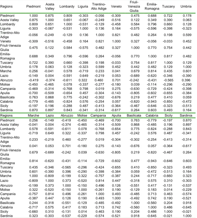
such relationship between the considered variables. Table 2 reports the proximity matrix arranged through the Pearson correlation coefficients () among the Regions.

Table 2: Proximity Matrix (Pearson coefficient of correlation )

Regions Piedmont Aosta

Valley Lombardy Liguria

Trentino-Alto Adige Veneto

Friuli-Venezia

Giulia

Emilia-Romagna Tuscany Umbria

Piedmont 1.000 0.875 0.809 -0.303 -0.056 -0.309 0.475 0.688 0.722 0.178 Aosta Valley 0.875 1.000 0.651 -0.067 -0.249 -0.516 0.122 0.349 0.390 0.063 Lombardy 0.809 0.651 1.000 -0.531 -0.129 -0.458 0.584 0.796 0.660 0.128 Liguria -0.303 -0.067 -0.531 1.000 0.136 0.164 -0.575 -0.596 -0.398 -0.323 Trentino-Alto Adige -0.056 -0.249 -0.129 0.136 1.000 0.821 0.482 0.264 0.198 0.599 Veneto -0.309 -0.516 -0.458 0.164 0.821 1.000 0.327 -0.056 -0.033 0.452 Friuli-Venezia Giulia 0.475 0.122 0.584 -0.575 0.482 0.327 1.000 0.770 0.754 0.442 Emilia-Romagna 0.688 0.349 0.796 -0.596 0.264 -0.056 0.770 1.000 0.817 0.482 Tuscany 0.722 0.390 0.660 -0.398 0.198 -0.033 0.754 0.817 1.000 0.129 Umbria 0.178 0.063 0.128 -0.323 0.599 0.452 0.442 0.482 0.129 1.000 Marche 0.256 -0.041 0.578 -0.719 0.233 0.041 0.679 0.814 0.435 0.601 Lazio -0.149 0.004 -0.591 0.649 -0.219 0.053 -0.689 -0.620 -0.346 -0.390 Abruzzo -0.419 -0.374 -0.611 0.322 0.460 0.701 -0.242 -0.431 -0.565 0.396 Molise -0.450 -0.465 0.078 -0.337 -0.277 -0.180 0.039 -0.114 -0.296 -0.290 Campania -0.469 -0.314 -0.768 0.798 0.019 0.275 -0.630 -0.729 -0.424 -0.398 Apulia -0.700 -0.509 -0.654 0.457 -0.304 -0.143 -0.805 -0.602 -0.655 -0.384 Basilicata 0.763 0.868 0.775 -0.242 -0.302 -0.676 0.219 0.477 0.410 0.059 Calabria -0.779 -0.485 -0.824 0.576 -0.254 0.057 -0.820 -0.943 -0.850 -0.472 Sicily -0.197 0.196 -0.288 0.487 -0.413 -0.364 -0.467 -0.646 -0.323 -0.513 Sardinia 0.870 0.897 0.843 -0.341 -0.314 -0.617 0.264 0.603 0.493 0.164

Regions Marche Lazio Abruzzo Molise Campania Apulia Basilicata Calabria Sicily Sardinia Piedmont 0.256 -0.149 -0.419 -0.450 -0.469 -0.700 0.763 -0.779 -0.197 0.870 Aosta Valley -0.041 0.004 -0.374 -0.465 -0.314 -0.509 0.868 -0.485 0.196 0.897 Lombardy 0.578 -0.591 -0.611 0.078 -0.768 -0.654 0.775 -0.824 -0.288 0.843 Liguria -0.719 0.649 0.322 -0.337 0.798 0.457 -0.242 0.576 0.487 -0.341 Trentino-Alto Adige 0.233 -0.219 0.460 -0.277 0.019 -0.304 -0.302 -0.254 -0.413 -0.314 Veneto 0.041 0.053 0.701 -0.180 0.275 -0.143 -0.676 0.057 -0.364 -0.617 Friuli-Venezia Giulia 0.679 -0.689 -0.242 0.039 -0.630 -0.805 0.219 -0.820 -0.467 0.264 Emilia-Romagna 0.814 -0.620 -0.431 -0.114 -0.729 -0.602 0.477 -0.943 -0.646 0.603 Tuscany 0.435 -0.346 -0.565 -0.296 -0.424 -0.655 0.410 -0.850 -0.323 0.493 Umbria 0.601 -0.390 0.396 -0.290 -0.398 -0.384 0.059 -0.472 -0.513 0.164 Marche 1.000 -0.809 -0.199 0.322 -0.757 -0.387 0.244 -0.717 -0.660 0.323 Lazio -0.809 1.000 0.373 -0.520 0.814 0.447 -0.318 0.575 0.310 -0.303 Abruzzo -0.199 0.373 1.000 -0.150 0.496 0.126 -0.551 0.417 -0.131 -0.537 Molise 0.322 -0.520 -0.150 1.000 -0.261 0.190 -0.129 0.183 0.014 -0.229 Campania -0.757 0.814 0.496 -0.261 1.000 0.493 -0.485 0.713 0.463 -0.574 Apulia -0.387 0.447 0.126 0.190 0.493 1.000 -0.492 0.742 0.190 -0.521 Basilicata 0.244 -0.318 -0.551 -0.129 -0.485 -0.492 1.000 -0.560 0.204 0.918 Calabria -0.717 0.575 0.417 0.183 0.713 0.742 -0.560 1.000 0.486 -0.645 Sicily -0.660 0.310 -0.131 0.014 0.463 0.190 0.204 0.486 1.000 -0.021 Sardinia 0.323 -0.303 -0.537 -0.229 -0.574 -0.521 0.918 -0.645 -0.021 1.000

Source: Istat data bank. Survey on the structure of farm production, 2013. http:/agri.istat.it

The adopted aggregation technique is the average bond in which the distance among groups of Regions is defined as the arithmetic average of the distances among all possible couples of Regions or groups of Regions (Forgy, 1965; MacQueen, 1967). The distance between two Regions or groups of Regions, d(i,h), was calculated through the Euclidean metric:

𝑑(𝑖, ℎ) = √∑ (𝑥𝑗 𝑖𝑗− 𝑥ℎ𝑗)2 (2)

In Table 2, as aforesaid, the highest positive values signify high similarity, whereas the lowest negative values indicate antinomy and then dissimilarity. Therefore, as example, the structural characters of the agricultural system of Piedmont is very similar to that one of Valle d'Aosta (0.875), whereas it is dissimilar from that of

(4)

Calabria (-0.779). Similarly the farms features of Aosta Valley are like those of Sardinia (+0.897), but are very different from those of Veneto (-0.516), and so on.

3. Results

3.1 The bundling into 6 groups

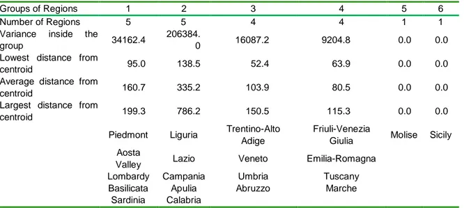
The results highlighted 6 groups of Regions as shown in Table 3. The first group comprised 5 Regions (Piedmont, Aosta Valley, Lombardy, Basilicata and Sardinia); the second group comprised 5 Regions (Liguria, Lazio, Campania, Apulia and Calabria); the third group included 4 Regions (Trentino Alto Adige, Veneto. Umbria and Abruzzo); the fourth group included three regions (Emilia Romagna, Tuscany and Marche), the latter two groups included only one Region: the fifth group Molise and Sicily the sixth one.

Table 3: Bundling parameters concerning the obtained 6 groups of Regions.

Groups of Regions 1 2 3 4 5 6

Number of Regions 5 5 4 4 1 1

Variance inside the

group 34162.4

206384.

0 16087.2 9204.8 0.0 0.0

Lowest distance from

centroid 95.0 138.5 52.4 63.9 0.0 0.0

Average distance from

centroid 160.7 335.2 103.9 80.5 0.0 0.0

Largest distance from

centroid 199.3 786.2 150.5 115.3 0.0 0.0

Piedmont Liguria Trentino-Alto Adige

Friuli-Venezia

Giulia Molise Sicily Aosta

Valley Lazio Veneto Emilia-Romagna

Lombardy Campania Umbria Tuscany

Basilicata Apulia Abruzzo Marche

Sardinia Calabria

The cartogram reported in Figure 1 points out that predominantly the groups of Regions comprise adjacent Regions but also some non-adjacent Regions and sometimes geographically distant ones.

.

Figure 1: Italy partitioned into 6 homogeneous groups of Regions.

The groups of Regions have different inside variability: obviously the groups formed by a single Region have nothing variability; the second group is the most heterogeneous, whereas the variability of the other three groups (first, third and fourth) is limited.

A synthetic evaluation about the obtained classification in 6 groups is given splitting the total variability into two parts: the one calculated inside the groups and the other one estimated among the groups. The classification is considered satisfactory if the variability among the groups is higher than that inside the groups. In the case

(5)

under study, almost 60 % of the total variability is recorded among the 6 groups that therefore appear well differentiated (Table 4).

Table 4: Splitting of the variance concerning the classification Source of variability Variance Percentage

Inside the groups 74147.3 40.2 Among the groups 110155.8 59.8

Overall 184303.1 100.0

3.2 Centroids of the groups analysis

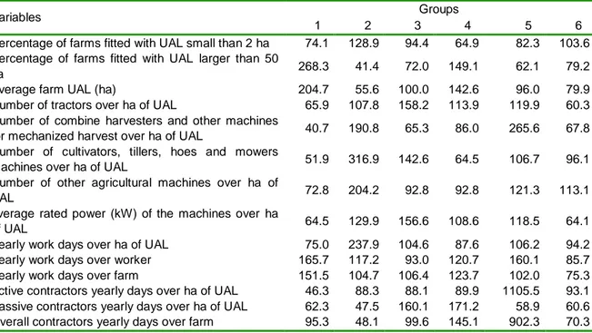
Table 5 reports for each group the centroids, that is the average values, of the considered variables, obtained from the analysis. These centroids, taking into account of the greater or lesser incidence of the values of the respective variables allow to define the features of each group.

It is clear that for the groups formed by a single Region the centroids matches with the values of the pertaining Regions.

Table 5 - Centroid of the considered variables for each group of Regions.

Variables Groups

1 2 3 4 5 6

Percentage of farms fitted with UAL small than 2 ha 74.1 128.9 94.4 64.9 82.3 103.6 Percentage of farms fitted with UAL larger than 50

ha 268.3 41.4 72.0 149.1 62.1 79.2

Average farm UAL (ha) 204.7 55.6 100.0 142.6 96.0 79.9

Number of tractors over ha of UAL 65.9 107.8 158.2 113.9 119.9 60.3

Number of combine harvesters and other machines

for mechanized harvest over ha of UAL 40.7 190.8 65.3 86.0 265.6 67.8

Number of cultivators, tillers, hoes and mowers

machines over ha of UAL 51.9 316.9 142.6 64.5 106.7 96.1

Number of other agricultural machines over ha of

UAL 72.8 204.2 92.8 92.8 121.3 113.1

average rated power (kW) of the machines over ha

of UAL 64.5 129.9 156.6 108.6 118.5 64.1

Yearly work days over ha of UAL 75.0 237.9 104.6 87.6 106.2 94.2

Yearly work days over worker 165.7 117.2 93.0 120.7 160.1 85.7

Yearly work days over farm 151.5 104.7 106.4 123.7 102.0 75.3

Active contractors yearly days over ha of UAL 46.3 88.3 88.1 89.9 1105.5 93.1 Passive contractors yearly days over ha of UAL 62.3 47.5 160.1 171.2 58.9 60.6

Overall contractors yearly days over farm 95.3 48.1 99.6 145.1 902.3 70.3

The first group is characterized by a significant number of large farms, i.e. fitted with UAL greater than 50 ha, and therefore also by a respectable average UAL. Furthermore the substantial impact of the yearly work days over both operator and farm is clear in this group.

The second group is typified by the large number of small farm, that is with UAL small than 2 ha, by a strong employment of mechanization, as well as by a large number of yearly work days over ha of UAL. The third group is individualized by the number of tractors over ha of UAL which is higher than the national average, as well as by the substantial average rated power (kW) of the machines over ha of UAL. Furthermore, it is also outstanding the passive contractors yearly days over ha of UAL. The fourth group is characterized by a hefty number of large farms higher than the national average and then high average UAL. Respectable is also to resort to labour, in particular passive contractors over ha of UAL and in any case to make use of overall contractors. The Molise (fifth group) is typified by the high value concerning the active contractors yearly days over ha of UAL, whereas the other variables are not far from the corresponding national averages. Aalso the Sicily (sixth group) is characterized by levels of the variables close to the corresponding national averages.

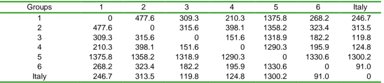
3.3 Distances of the groups centroids by each other and by the national centroid

Table 6 reports the distances of the groups centroids by each other and by the national centroid, measured through equation (2). For example, the first group of Regions is very close to the fourth group (210.3) and far from the fifth, that is the Molise (1375.3). Conversely, the second group is near the third one (315.6) and the

(6)

farthest is still the Molise (1358.2). The two closest groups of Regions are the third and fourth (151.6), the two most distant groups are the first one and Molise (1375.8).

Table 6 - Distances of the groups centroids by each other and by the national centroid

Groups 1 2 3 4 5 6 Italy 1 0 477.6 309.3 210.3 1375.8 268.2 246.7 2 477.6 0 315.6 398.1 1358.2 323.4 313.5 3 309.3 315.6 0 151.6 1318.9 182.2 119.8 4 210.3 398.1 151.6 0 1290.3 195.9 124.8 5 1375.8 1358.2 1318.9 1290.3 0 1330.6 1300.2 6 268.2 323.4 182.2 195.9 1330.6 0 91.0 Italy 246.7 313.5 119.8 124.8 1300.2 91.0 0

4. Conclusions

The arrangement of the Italian Regions into six groups, taking into account the size of the farms, their agricultural mechanization level and the manpower employment, showed clear picture of the structure of the Italian farms.

The first group of Regions (the ones of North-West, Sardinia and Basilicata) is characterized by a significant number of large farms and a considerable impact of the yearly work days over both operator and farm. The second group (Southern Regions and Lazio, except Basilicata) is characterized by the high presence of small farm, as well as by a large number of yearly work days over ha of UAL. The third group (Trentino Alto Agige, Veneto, Umbria and Abruzzo) is typified by the great number of tractors over ha of UAL and the high passive contractors yearly days over ha of UAL. The fifth group (Molise) is characterized by high mechanization levels and large active contractors yearly days over ha of UAL. The fourth (Emilia-Romagna, Tuscany, Marche and Friuli-Venezia Giulia) and the sixth group (Sicily) have less distinct characteristics and the values of all the variables very close to the corresponding national averages.

Acknowledgments

Simone Pascuzzi and Lucia Mongelli conceived and designed the study. Lucia Mongelli studied and interpreted the data, performed the statistical analysis and wrote the paper.

Reference

CREA, 2016. Report sullo stato dell'arte dell'agricoltura di precisione in Italia: sintesi della chiamata per contributi di ricerca ed innovazione. Consiglio per la Ricerca in agricoltura e l'analisi dell'Economia Agraria (CREA), Rome, Italy

Forgy E.W., 1965. Cluster analysis of multivariate data: efficiency versus interpretability of classifications. Biometrics 21, pag. 768-769.

Forleo M., 2001. Strumenti per la progettazione di politiche per lo sviluppo dei sistemi agricoli locali di Calabria e Puglia. La Puglia. Analisi delle caratteristiche degli ambiti agricoli sub-regionali. INEA, Programma Operativo Multiregionale. Attività di sostegno ai servizi di sviluppo per l’agricoltura. Misura 2. Università della Calabria.

Istat, 2017. Agricoltura e zootecnia. Struttura delle aziende agricole 2013. Banca dati Istat. http:/agri.istat.it MacQueen J. B., 1967. Some Methods for classification and Analysis of Multivariate Observations,

Proceedings of 5-th Berkeley Symposium on Mathematical Statistics and Probability, Berkeley, University of California Press, 1, pag. 281- 297.

Pascuzzi S., 2013. The effects of the forward speed and air volume of an air-assisted sprayer on spray deposition in “tendone” trained vineyards. J. of Ag. Eng., 3:125-132.

Pascuzzi S., 2015. A multibody approach applied to the study of driver injures due to a narrow-track wheeled tractor rollover. J. Agric. Eng., 46:105-114.

Pascuzzi S., Santoro F., 2015. Exposure of farm workers to electromagnetic radiation from cellular network radio base stations situated on rural agricultural land. International Journal of Occupational Safety and Ergonomics, 21(3):351–358.

Pascuzzi S., Santoro F., 2017. Evaluation of farmers’ OSH hazard in operation nearby mobile telephone radio base stations". 16th International Scientific Conference "Engineering for rural development". Proceedings, Volume 16. Jelgava, Latvia, May 24-26, 2017, pp. 748-755 – ISSN: 1691-5976 DOI: 10.22616/ERDev2017.16.N151