energies
ISSN 1996-1073 www.mdpi.com/journal/energies Article
Estimation of Downtime and of Missed Energy Associated with
a Wave Energy Converter by the Equivalent Power Storm Model
Felice Arena 1,2,*, Valentina Laface 1,†, Giovanni Malara 1,2,† and Alessandra Romolo 1,2,† 1 Natural Ocean Engineering Laboratory (NOEL), “Mediterranea” University of Reggio Calabria,
Loc. Feo di Vito, Reggio Calabria 89122, Italy; E-Mails: [email protected] (V.L.); [email protected] (G.M.); [email protected] (A.R.)
2 Wavenergy.it srl. Via F. Baracca Trav. De Salvo 8/A, Reggio Calabria 89123, Italy
† These authors contributed equally to this work.
* Author to whom correspondence should be addressed; E-Mail: [email protected]; Tel.: +39-0965-1692-260; Fax: +39-0965-1692-201.
Academic Editor: John Ringwood
Received: 1 September 2015 / Accepted: 10 October 2015 / Published: 15 October 2015
Abstract: The design of any wave energy converter involves the determination of relevant statistical data on the wave energy resource oriented to the evaluation of the structural reliability and energy performance of the device. Currently, limited discussions concern the estimation of parameters connected to the energy performance of a device. Thus, this paper proposes a methodology for determining average downtime and average missed energy, which is the energy that is not harvested because of device deactivations during severe sea storms. These quantities are fundamental for evaluating the expected inactivity of a device during a year or during its lifetime and are relevant for assessing the effectiveness of a device working at a certain site. For this purpose, the equivalent power storm method is used for their derivation, starting from concepts pertaining to long-term statistical analysis. The paper shows that the proposed solutions provide reliable estimations via comparison with results obtained by processing long wave data.
Keywords: wave power; long-term statistics; downtime; missed energy; wave energy converters
1. Introduction
Past and recent works proved that the wave energy resource might contribute significantly to the supply of electrical energy on a global scale. Indeed, this resource has the potential for providing from 16,000 TWh/y to 32,000 TWh/y offshore wave energy, which is remarkable even if the exploitable limit is about 10%–20% [1,2]. The efforts of several research groups were oriented toward the determination of the most attractive sites and of the most reliable technologies for wave energy exploitation. The former analyses were conducted in several areas, such as the Mediterranean Sea [3–9], the Black Sea [10,11], the USA [12–14] and in various Asian regions [15–17]. The latter analyses involved the conception of a variety of devices and theoretical and experimental tests on both small-scale and full-scale devices [18–20]. In this regard, irrespective of their specific working principle, a general requirement for all devices is to define working conditions and energy performance in the light of prescribed safety regulations. These restrictions comprise the deactivation of the devices during the occurrence of severe wave conditions. Thus, it is extremely important to provide estimates on the expected time during which a device is deactivated (downtime) and the expected amount of energy that is not harvested during that time (missed energy). Indeed, these quantities are relevant for assessing the energetic performance and economic feasibility of any device.
The estimation of downtime and of missed energy relies on wave data statistical analysis that is commonly adapted from applied statistics methodologies and from marine engineering applications, where the so-called “persistence” is the analogue of the downtime [21]. In this context, the common approach to the problem is distinguishing sea wave behavior by two time scales: the short time scale (~hours); and the long time scale (~years). The former is analyzed by analytical models based, usually, on the representation of the linear free surface displacement as a stationary ergodic Gaussian process (the sea state) [22], which is applied to wave records of 0.5 h. The latter is analyzed via statistics associated with single realizations of recorded sea states and accounts for the non-stationary character of the sea waves. In this case, investigations involve both models and data processing, and this is the framework under which the downtime and the missed energy are calculated.
An approach proposed by some authors is to relate persistence statistics to wave conditions. Specifically, Houmb [23] described sea storm events by a Poisson model leading an exponential distribution of storm persistence. Houmb and Vik [24] developed a model for determining both the duration of extreme events and “calms” between them. They dropped the Poisson model and proposed the use of a two-parameter Weibull distribution. Graham [25] proposed a model incorporating the concepts introduced in the previous works, that is that the occurrence of persistence durations may be defined in terms of a Weibull distribution. His approach is based on the idea of parameterizing persistence statistics in order to connect the sea state probability of exceedance with the persistence. Kuwashima and Hogben [26] further developed Graham’s approach by providing a model that is simpler, more reliable and applicable also when reliable measured data are not available. Others approaches are those of Anastasiou and Tsekos [27,28] an providing the estimation of persistence statistics in the framework of Markov processes, both in discrete time and in continuous time.
A quite different approach for modelling the non-stationary character of the sea waves is the equivalent storm model (ESM) [21,29,30]. It is applied starting from an appropriately long significant wave height (Hs) time history, from which recorded storms are identified. The method involves the
replacement of each storm with a fictitious storm having a prescribed (parameterized) time variation, which is equivalent to the real one in a certain statistical sense. Such a replacement allows constructing an “equivalent sea”, that is a sequence of equivalent storms, which is used for deriving relevant wave statistics and has the crucial feature of providing an analytical solution for the determination of the storm peak distribution, thus circumventing the best fit of the data. In this regard, it is worth mentioning that this approach allowed deriving closed-form solutions for the calculation of return values of interest in structural reliability analysis, such as the return period of significant wave heights, of individual wave heights and of nonlinear crest heights [31–33]. Further, it provided simple expressions for the determination of average persistence above a certain significant wave height threshold, which are not yet validated against recorded data. The ESM was applied in the open literature via piecewise linear and power law models. The former is known as equivalent triangular storm (ETS), the latter as equivalent power storm (EPS). In this regard, note that the EPS is a generalization of the ETS.
The objective of this paper is to provide simple and widely-applicable formulae for the calculation of both downtime and missed energy. For this purpose, the EPS model is exploited. Specifically, the paper shows that it can be used for estimating downtime and missed energy associated with both single storm realizations and storm sequences. The reliability of these results is assessed against results obtained by processing long recorded wave data.
2. Mathematical Background
This section summarizes the crucial characteristics of the EPS model and results relevant for the objective of the paper.
The EPS is implemented starting from Hs records allowing the identification of sea storms. For this purpose, the definition of sea storm proposed by Boccotti [21] is adopted. Specifically, a sea storm is a sequence of sea states during which the significant wave height Hs exceeds a certain threshold hcrit and does not fall below it for a certain time interval ΔT. Usually, the time interval is 12 h, while the threshold hcrit is related to the recorded average significant wave height <Hs>. Thus, it depends on the characteristics of the recorded sea states at the considered site. Boccotti proposed a threshold value hcrit equal to 1.5<Hs>.
2.1. The Equivalent Power Storm Model
Starting from a storm record composed of a sequence of sea states of given significant wave height Hs and mean spectral period Tm, the associated EPS is constructed by representing the Hs time variation within each storm via the following equation:
0 2 ( ) 1 t t h t a b , for t0 − b/2 ≤ t ≤ t0 + b/2 (1)
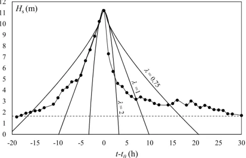
where t0 is the time instant associated with the maximum recorded Hs, a and b are the intensity and duration of the EPS and λ is a positive definite free parameter determining the shape of the EPS. Considering different values of the λ parameter, different storm shapes are produced. For instance,
for λ = 0.75, 1, 2 cusp, triangular and parabolic storms are constructed (Figure 1). It is readily seen that by this model the time spent above a threshold h is given by the equation:
1/ EPS( , , , ) 1 h t h a b b a (2)
It is noteworthy that, by enforcing an equality between the first order moments, we should expect that the Hmax distributions are different from each other. Nevertheless, it was seen by processing hundreds of data that even the distributions are quite close to each other. Thus, real storm statistics can be investigated by their EPS counterparts, as they are equivalent in a probabilistic sense [21,29–33].
Figure 1. Storm recorded by the 42001 buoy and related equivalent power storms (EPSs) for λ = 0.75, 1, 2.
The EPS shape is commonly determined a priori. The a parameter is assumed equal to the maximum recorded Hs of the storm. The b parameter is calculated by enforcing an equality between the first order moments of the random variables Hmax, which is the maximum individual crest-to-trough wave height associated with a storm realization, pertaining to the recorded storm and to the EPS. This specific computation is pursued via the Borgman [34,35] approach, which allows estimating the probability of the exceedance of the random variable Hmax and deriving the equations:
max m 0 0 ln ( ( )) 1 exp d d ( ( )) D H F x t H t H T x t
(3)where ( )F x is the cumulative distribution of the crest-to-trough wave height (H) pertaining to a sea H state with significant wave height Hs = x [21,36,37] and:
max 1 1 m 0 0 1 ( , ) 1 exp ln ( ) 1 d d ( ) a H b x H a b F x x H a T x a
(4) 0 1 2 3 4 5 6 7 8 9 10 11 12 -20 -15 -10 -5 0 5 10 15 20 25 30 Hs (m) t-t0(h)that are used for estimating the first order moments, respectively, via wave data and the EPS model. The cumulative distribution of Boccotti [38] can be used for the calculations. It is given by the equation:
2 4 ( ) 1 exp 1 * H H F x x (5)
ψ* being the ratio between the absolute minimum and the absolute maximum of the autocovariance function of the free surface displacement associated with a certain sea state [21].
2.2. Return Period of Significant Wave Height R(h) and Mean Persistence Dm(h) above a Threshold h
By applying the EPS concept to the entire storm sequence recorded at a certain site, the model can be used for estimating the storm peak distribution. In this regard, the procedure described by Fedele and Arena [30] is characterized by the fact that this distribution is derived analytically by imposing that the average time during which Hs is above a certain threshold h for the recorded storm sequence and the EPS sequence is equal. Thus, it is derived by imposing a stochastic equivalence between the real sea and the equivalent sea, in which the recorded data are required only for estimating cumulative distributions of significant wave height FHs(x) and average conditional (to the storm peak a) EPS
duration ( )b a . In this framework, the return period of significant wave height R(h) is calculated by the following equation: 1 ( ) 1 ( , )d ( ) h R h G a a b a
(6)where G(λ,a) is defined as:
2 1/ 2 1 , 2 2 2 1 2 1 , d ( ) sin( / ) ( ) d ; 1 / d d ( ) ( , ) ; 1 d d ( ) ( 1) sin( ) ( 1) d ; ( ) 1 ! d s s s H a x H n n n H n a x F z x a x if z F a G a if a F z a x x if n n z
(7)with integer n > 1 and 0 < μ < 1.
The calculation of the average downtime Dm(h) (or, equivalently, persistence) proceeds directly from this result. Indeed, it is defined as the ratio between the total time interval in which Hs is above h during a long time span τ and the number of storms N(h) whose maximum significant wave height is greater than h occurring during τ. Considering that the total time in which Hs is above h is τ[1 − FHs(h)]
and N(h) = τ/R(h), then:
s
m( ) ( )[1 H ( )]
D h R h F h (8)
If a linear law (λ = 1) is used for describing the EPS storm history in the time domain and a three-parameter Weibull distribution is assumed for
s( )
H
1 ( ) ( ) exp 1 u l u l u h h b h R h w h h h u w w (9) and: m 1 ( ) ( ) 1 u l u b h D h h h h u w w (10)
where u, w and hl are parameters of the Weibull distribution:
s( ) 1 exp u l H h h F h w (11)
In this context, the parameter w is a scale parameter, u is a parameter rendering a quantification of the significant wave height associated with different probability thresholds and hl is a location-dependent parameter.
3. Theoretical Derivation of the Missed Energy during Sea Storms
In this section, the EPS model is used for deriving analytical formulae for the calculation of the missed energy ΔEEPS during sea storms. The calculation is pursued by concentrating first on the single storm event and then on the storm sequence. In this last case, the average energy missed by deactivating a device during the occurrence of storms with Hs greater than a certain threshold htr is given.
3.1. Storm Energy and Missed Energy via the Equivalent Power Storm (EPS) Model
The expression of the wave energy associated with a given EPS (EEPS) is derived starting from the calculation of the energy of an actual storm (EAS). The energy of a sea storm is obtained by cumulating the wave power contribution of each sea state. Specifically, denoting D the storm duration, we have that:
AS 0
( )d
D
E
t t (12)where φ(t) is the wave power propagated by the sea state. The deep water wave power in a sea state is calculated via the equation [8]:
2 2 s f m 64 g H T (13)
where ρ is the water density, g is the acceleration due to gravity and γf is a frequency-dependent parameter. Equation (13) is simplified further by considering that the mean wave period Tm can be related directly to the significant wave height Hs. Indeed, Arena et al. [39] showed that:
s m m( PH, ) H T K g (14)
Km(αPH,γ) being a constant dependent on the spectral shape of the free surface displacement through the Phillips’ parameter αPH and the JONSWAP peak enhancement factor γ [40]. Equation (14) is an approximation that is reliable for large Hs values [33]. Therefore, it can be adopted in our contexts, as wave energy converters are expected to be deactivated during extreme wave conditions. The variation of Km(αPH,γ) is quite limited. Indeed, it varies over the interval [8.5, 11.4] for a wide range of the Phillips’ parameter (0.008, 0.022) and of the peak enhancement factor (0.5, 6). Similar considerations hold for the γf parameter. Indeed, it has a quire restricted variability, as it is equal to 1.12 for the mean JONSWAP spectrum and to 1.15 for the Pierson–Moskowitz spectrum [41] and is also irrespective of the significant wave height Hs. Thus, Equation (13) can be reduced for being dependent only on Hs for a specified frequency spectrum. Specifically:
2.5 s kH (15) where: 1.5 f m( PH, ) 64 g k K (16)
The adequacy of this approximation was assessed by Arena et al. [8]. They showed that introducing a JONSWAP-like approximation on the frequency spectrum allows obtaining reliable results for the calculation of the wave power even in case of bimodal seas.
The EPS model is here exploited for calculating integral in Equation (12) in a simplified form. Indeed, considering the given time history of the EPS and its symmetry with respect to t = t0 (that, without loss of generality, may be assumed t0 = 0), integral in Equation (12) is expressed from time domain to the height domain in the form:
EPS crit 1 2.5 1 1.5 crit ( , , , ) 1 d a h b h h E a b h ka h a a
(17)Equation (17) is applicable for any value of the shape parameter λ. However, it is worth noting that if a triangular (λ = 1) shape is considered, a quite simple result is obtained:
EPS 3.5 3.5 crit crit ( , , ,1) 3.5 k b E a b h a h a (18)The proposed expressions are quite versatile and simple to apply. Indeed, relying on predetermined storm time variations allows utilizing Equations (17) and (18) directly for the calculation of the missed energy. For this purpose, it is sufficient to observe that, in real contexts, a wave energy converter is expected to operate until the significant wave height reaches a threshold htr, which is certainly larger than hcrit. Therefore, missed energies are estimated by setting the lower bound of integration in Equation (17) to htr. In addition, note that by setting the lower bound to hcrit, the total energy associated with the given storm is obtained.
3.2. Average Missed Energy for Given Sequences of Sea Storms
Wave energy converters are expected to survive for several years. Therefore, a relevant parameter for assessing their long-term adequacy is the average amount of missed energy due to sea storm sequences occurring during the device lifetime.
Given a certain storm sequence occurring during a long time τ and a device that is deactivated if the significant wave height is larger than htr in the storms exceeding htr, the average missed energy ΔEm(htr) is obtained as the ratio between the total energy ETOT(htr) missed by the device and the number N(htr) of storms whose maximum Hs exceeds htr during τ:
TOT tr m tr tr ( ) ( ) ( ) E h E h N h (19) Considering that: s tr TOT( )tr ( ) H ( )d h E h h p h h
(20)pHs(h) being the significant wave height probability density function, and: tr tr ( ) ( ) N h R h (21) then: s tr m( )tr ( )tr ( ) H ( )d h E h R h h p h h
(22)Equation (22) holds irrespective of the storm shape and is applicable from recorded storm sequences. However, if R(htr) is calculated by Equation (6), it provides the average missed energy ΔEm associated with EPS sequences.
The behavior of Equation (22) for EPSs with shape parameter λ = 1 is shown in Figure 2 (the required input parameters are presented in detail in Section 4 considering buoy data of 42001). The figure shows that ΔEm has a bell-shaped trend. Specifically, it is increasing for values of htr less than 20 m and is decreasing for higher htr thresholds. This behavior relates to the fact that the pHs(h)
decaying compensates the R(htr) growing pattern only for large significant wave height values. It is worth mentioning that thresholds larger than 10–15 m have no practical relevance. Therefore, the missed energy ΔEm may be considered in realistic applications as an increasing function of htr (Figure 2, continuous line). The maximum is dependent on the specific site under investigation. However, the pattern shown in Figure 2 is general.
This result seems to contradict the intuitive idea that a device working at larger thresholds is able to harvest more energy and, thus, reduces the missed energy. This intuitive concept is correct as long as the storm concept is not invoked. Indeed, in this last case, the average number of storms contributes significantly to the calculation of the missed energy and is responsible for the resulting behavior.
Figure 2. Theoretical trend of average missed energy above a given threshold h in the EPSs with maximum Hs greater than h.
4. Numerical Results: Reliability of the Proposed Expressions
In this section, the results proposed in Section 3 are applied considering wave data recorded in the Gulf of Mexico by the 42001 buoy of NOAA-NDBC (National Oceanic and Atmospheric Administration’s National Data Buoy Center) and in the Pacific Ocean by the 46006 buoy (Figure 3). The data were recorded from August 1975–December 2012, giving rise to a set of 281.970 data for the 42001 buoy, while, in the other case, data were recorded from April 1977 to February 2013 giving rise to a dataset of 231.056 samples. The calculation of downtime and of missed energy above a given significant wave height threshold is performed both for individual storms and for a given storm sequence. The main objective of the analysis is to compare results obtained by applying the EPS model to analogous quantities calculated from actual storm time histories, in order to assess the reliability of the proposed methodology for wave energy calculations.
Figure 3. Locations of the buoys 46006 and 42001. 0 1000 2000 3000 4000 5000 6000 7000 8000 0 10 20 30 40 50 60 70 80 90 100 110 120 130 140 150 ∆ Em (k W h/ m ) h (m) λ = 2 λ = 1 λ = 0,75 46006 (40.754 N, 137.464 W) North Atlantic Ocean Gulf of Mexico North Pacific Ocean 1000 km N E S W Gulf of Alaska 42001 (25.888 N, 89.658 W)
4.1. Preliminary Calculation of Wave Data Statistics
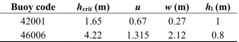
The analysis carried out in this section requires the estimation of the parameters of the significant wave height distribution and of the average conditional base ( )b a . In both cases, a mean square minimization procedure is used for the calculation. Specifically, for the three-parameter Weibull distribution of Equation (11), the values summarized in Table 1 are calculated. For the average conditional base ( )b a , the calculation is pursued by the approach proposed by Arena and Pavone [29], which approximates the conditional base with a mean base calculated from the processed data. The parameters are given in Table 2 for EPS with various λ values.
It is seen that the locations have quite different wave climate conditions. Indeed, the critical significant wave height threshold htr and the scale parameter w are significantly larger in the Pacific Ocean, while less significant variations are observed for the other parameters.
Table 1. Parameters of the cumulative distribution FHs(h) and significant wave height
threshold chosen for storm identification hcrit.
Buoy code hcrit (m) u w (m) hl (m)
42001 1.65 0.67 0.27 1
46006 4.22 1.315 2.12 0.8
Table 2. Mean base associated with different EPSs.
Buoy Code λ b (h) 42001 0.7 237,308 0.75 188,608 1 82,551 2 25,096 46006 0.7 238,442 0.75 190,368 1 84,450 2 26,139
4.2. Downtime and Energy Associated with a Single Storm Realization
Given the recorded storm sequences, the EPS associated with each storm is calculated for various λ values. Specifically, the energy of each storm EAS is evaluated by Equation (12) and compared to the EPS counterpart (EEPS) provided by Equation (17) or (18). Figure 4 shows the comparison between EAS and EEPS. Each point pertains to the realization of a recorded storm for the particular case in which λ = 1. The figure shows that the model may both overestimate and underestimate the measured quantities. Thus, a measure of the scatter between data and results is used for quantifying the error. Specifically, the following error is estimated:
AS, EPS, 1 AS, 1 N i i i i E E N E
(23)N being the number of storms and i denoting the i-th storm record. The results of the calculation are shown in Figure 5, which involves errors associated with the use of different EPS shapes. In this
regard, it is seen that the λ choice affects the quality of the calculation. Indeed, the best estimates are achieved by adopting a λ < 1. However, moderate variations are observed in the vicinity of the shape leading to the smallest error, which are confined to 10%–20%.
(a) (b)
Figure 4. Wave energy pertaining to single storm realizations (EAS) versus theoretical values (EEPS) calculated by the EPS model with λ = 1: (a) the buoy 42001; and (b) the buoy 46006.
(a) (b)
Figure 5. Error in Equation (23) calculated for various storm shapes from data (a) of the buoy 42001 and (b) of the buoy 46006.
Similar characteristics are observed in the calculation of the missed energy. For this purpose, the calculation is pursued by considering thresholds htr, which are a fraction of the storm peak. Specifically, the energy missed in each storm under the assumption that htr is 0.5-, 0.65- and 0.8-times the storm peak is calculated via storm data and Equation (17). Then, the error defined by Equation (23) is estimated. Figure 6 shows the error for the various EPS shapes. Even in this case, the influence of the λ parameter is relevant, but a comparison between the various data emphasizes the fact that good estimates, on average, are achieved by restricting the EPS model to λ < 1. In this regard, the crucial
1 10 100 1000 10000 1 10 100 1000 10000 EEP S (kW h/m ) EAS (kWh/m) 1 10 100 1000 10000 100000 1 10 100 1000 10000 100000 EEP S (kW h/m ) EAS (kWh/m) -1 -0.8 -0.6 -0.4 -0.2 0 0.2 0.4 0.6 0.8 1 0.75 0.8 0.85 0.9 0.95 1 1.5 2 ε λ -1 -0.8 -0.6 -0.4 -0.2 0 0.2 0.4 0.6 0.8 1 0.7 0.75 0.8 0.85 0.9 0.95 1 1.5 2 ε λ
feature of the model relates to the fact that an optimal λ can be identified via comparisons with data. Then, it can be adopted for pursuing the long-term statistical analyses. Analogous trends are observed for the downtime. This quantity is calculated via Equation (2), and errors of the form given by Equation (23) are estimated and shown in Figure 7. In this context, it is worth noting that they are coherent with the errors shown in Figure 6. Thus, optimal λ at a certain location are close to each other considering either the missed energy or the downtime.
(a) (b)
Figure 6. Error in Equation (23) calculated considering energies above a certain fraction of the storm peak for various EPS shapes: (a) the buoy 42001; and (b) the buoy 46006.
(a) (b)
Figure 7. Error in Equation (23) associated with the downtime pertaining to three fractions of the storm peak for various EPS shapes: (a) the buoy 42001; and (b) the buoy 46006.
Additional considerations may be drawn by comparing the performance of the EPS model at various thresholds htr. An apparent feature of all EPSs is that the error in calculating both the missed energy and the downtime via the EPS model decreases for increasing values of htr. This is connected to the agreement between the real storm shape and the EPS shape in the vicinity of the storm peak. Indeed, typical storm records pertaining to exceptional events are characterized by peaks with rapid growing and decaying patterns. Because of its geometrical structure, even the EPS has this specific feature. Thus, for quite large htr thresholds, EPSs “trace” recorded sea storms (in this regard, note that the EPS
-1 -0.8 -0.6 -0.4 -0.2 0 0.2 0.4 0.6 0.8 1 0.7 0.75 0.8 0.85 0.9 0.95 1 1.5 2 0.5 0.65 0.8
ε
λ
-1 -0.8 -0.6 -0.4 -0.2 0 0.2 0.4 0.6 0.8 1 0.7 0.75 0.8 0.85 0.9 0.95 1 1.5 2 0.5 0.65 0.8ε
λ
-1 -0.8 -0.6 -0.4 -0.2 0 0.2 0.4 0.6 0.8 1 0.7 0.75 0.8 0.85 0.9 0.95 1 1.5 2 0.5 0.65 0.8ε
λ
-1 -0.8 -0.6 -0.4 -0.2 0 0.2 0.4 0.6 0.8 1 0.7 0.75 0.8 0.85 0.9 0.95 1 1.5 2 0.5 0.65 0.8ε
λ
and real storm have the same peak amplitude a). This intuitive tendency is not confirmed, in general, by error in Equation (23), as it is seen in Figures 6 and 7 that this is not verified for some shape parameters. 4.3. Average Downtime and Average Missed Energy in a Sequence of Sea Storms
The storm sequences recorded by the buoys 42001 and 46006 are analyzed with the objective of estimating the average downtime and the average missed energy. In this regard, the crucial comparison is pursued between estimates of Equations (8) and (22) computed via the data and via the proposed equations.
The estimation is conducted starting from the synthetic parameters summarized in the Tables 1 and 2 for a number of EPS shapes. The integration involved in the computations is pursued by a quadrature scheme based on the midpoint rule. The calculation from data is accomplished directly from the storm time histories. Specifically, given the storm time histories, the total time spent by all sea storms over a given threshold is estimated. Then, the outcome is divided by the number of storms recorded by the buoy.
Figure 8 shows the average downtime calculated from the data (circles) and from Equation (8). It is seen that the EPS model is able to cover a wide range of values based on the values assigned to λ. Indeed, the smaller λ, the larger the downtime. This is a general characteristic of the model and relates to the fact that the storm duration (for a prescribed storm peak) is a decreasing function of the λ parameter. In terms of agreement with recorded data, it is seen that the EPS model is able to capture the qualitative behavior of this quantity over the entire h domain. However, for obtaining reliable estimates, the storm shape must be restricted to the λ belonging to the interval [0.7, 1]. Similar considerations hold for the missed energy.
(a) (b)
Figure 8. Comparison between mean persistence Dm above the threshold h in actual sea (circles) and in EPSs (continuous lines) having various storm shapes λ: (a) the buoy 42001; and (b) the buoy 46006.
Figure 9 shows a comparison among average missed energies, where circles denote data from records and continuous lines pertain to theoretical estimations. In both cases, comparisons are restricted to significant wave height thresholds associated with at least 10 storm records. For larger thresholds, the limited number of available storms does not allow estimating reliable statistics.
0 5 10 15 20 25 30 35 40 45 2 3 4 5 6 Dm (hours) h (m) λ = 2 0 5 10 15 20 25 30 35 40 45 4 5 6 7 8 9 10 11 Dm (hours) h (m) λ = 2 Dm (h) Dm (h)
(a) (b)
Figure 9. Comparison between average missed energy ΔEm above the threshold h in actual sea (circles) and in EPSs (continuous lines) having various storm shapes λ: (a) the buoy 42001; and (b) the buoy 46006.
5. Conclusions
The paper has discussed the problem of estimating quantities useful at the design stage of wave energy converters. Usually, these kinds of devices are expected to work under severe sea wave conditions that may involve their deactivation. Therefore, it is important to provide the estimation of the durations of these extreme storm events (downtime) and of the amount of energy missed during these events. In the paper, by relying on the concept of equivalent power storm, formulae for calculating the downtime and the missed energy above a given threshold are developed. The methodology can be applied to single storm events, as well as to storm sequences. In this context, the only input data are the significant wave height distribution and an empirical base-height regression for calculating the EPS duration b given the storm peak a.
The reliability of the proposed formulae has been assessed against data recorded in the Gulf of Mexico and in the Pacific Ocean. The analysis has been carried out considering EPSs with various shape parameters. It has been shown that reliable estimates may be obtained by selecting an appropriate value of the shape parameter. Indeed, estimations of the average error show that this quantity can be minimized for shape parameters ranging over the interval [0.7, 1]. The EPS method is shown to be reliable also for estimating the average downtime and the average missed energy. Indeed, there is a good agreement between the data and model results for the considered EPS shapes.
Acknowledgments
This paper has been developed during the Marie Curie project “PLENOSE” funded by European Union (Grant Agreement Number: PIRSES-GA-2013-612581).
Giovanni Malara is grateful to the Chamber of Commerce of Reggio Calabria for funding his activity by the post-doctoral fellowship “Sostenere l’occupazione per sostenere la Crescita”.
0 1000 2000 3000 4000 5000 6000 7000 8000 9000 10000 2 3 4 5 6 ∆Em (kWh/m) h (m) 0 1000 2000 3000 4000 5000 6000 7000 8000 9000 10000 4 5 6 7 8 9 10 11 ∆Em (kWh/m) h (m) λ = 1 λ = 2
Conflicts of Interest
The authors declare no conflict of interest. Nomenclature
a storm intensity of EPS b storm duration of EPS
( )
b a base-height regression function D actual storm duration
Dm(h) mean persistence above the threshold h EAS actual storm energy
( )
H
F x cumulative distributions of significant wave height EEPS EPS storm energy
ETOT(htr) total missed energy
g acceleration due to gravity
H individual crest-to-trough wave height hcrit significant wave height critical threshold
Hmax maximum individual crest-to-trough wave height associated with a storm realization max
H maximum expected wave height Hs significant wave height
htr significant wave height threshold
N(htr) number of storms whose maximum Hs exceeds htr during a long time interval τ
pHs(h) significant wave height probability density function
t time instant
u, w, hl parameters of the significant wave height distribution
R(h) return period of a sea storm whose maximum Hs exceeds the threshold h Tm mean spectral period
t0 time instant at the maximum significant wave height Hs max for EPS αPH Phillips’ parameter
λ shape parameter
γ JONSWAP peak enhancement factor ϕ deep water wave power in a sea state
ρ water density
ΔEEPS missed energy for a given EPS ΔEm(htr) average missed energy
*
ratio between the absolute minimum and the absolute maximum of the autocovariance function of the free surface displacement associated with a certain sea state
References
1. Reguero, B.G.; Losada, I.J.; Méndez, F.J. A global wave power resource and its seasonal, interannual and long-term variability. Appl. Energy 2015, 148, 366–380.
2. Cruz, J. Ocean Wave Energy: Current Status and Future Perspectives; Springer: Heidelberg, Germany, 2008.
3. Iglesias, G.; López, M.; Carballo, R.; Castro, A.; Fraguela, J.A.; Frigaard, P. Wave energy potential in galicia (NW Spain). Renew. Energy 2009, 34, 2323–2333.
4. Iglesias, G.; Carballo, R. Wave energy potential along the Death Coast (Spain). Energy 2009, 34, 1963–1975.
5. Iglesias, G.; Carballo, R. Wave energy resource in the Estaca de Bares area (Spain). Renew. Energy 2010, 35, 1574–1584.
6. Iglesias, G.; Carballo, R. Offshore and inshore wave energy assessment: Asturias (N spain). Energy 2010, 35, 1964–1972.
7. Liberti, L.; Carillo, A.; Sannino, G. Wave energy resource assessment in the Mediterranean, the Italian perspective. Renew. Energy 2013, 50, 938–949.
8. Arena, F.; Laface, V.; Malara, G.; Romolo, A.; Viviano, A.; Fiamma, V.; Sannino, G.; Carillo, A. Wave climate analysis for the design of wave energy harvesters in the Mediterranean Sea. Renew. Energy 2015, 77, 125–141.
9. Silva, D.; Rusu, E.; Soares, C. Evaluation of various technologies for wave energy conversion in the Portuguese nearshore. Energies 2013, 6, 1344–1364.
10. Akpınar, A.; Kömürcü, M.İ. Assessment of wave energy resource of the Black Sea based on 15-year numerical hindcast data. Appl. Energy 2013, 101, 502–512.
11. Rusu, L. Assessment of the wave energy in the Black Sea based on a 15-year hindcast with data assimilation. Energies 2015, 8, 10370–10388.
12. Defne, Z.; Haas, K.A.; Fritz, H.M. Wave power potential along the atlantic coast of the southeastern USA. Renew. Energy 2009, 34, 2197–2205.
13. Stopa, J.E.; Cheung, K.F.; Chen, Y.-L. Assessment of wave energy resources in Hawaii. Renew. Energy 2011, 36, 554–567.
14. Lenee-Bluhm, P.; Paasch, R.; Özkan-Haller, H.T. Characterizing the wave energy resource of the US Pacific Northwest. Renew. Energy 2011, 36, 2106–2119.
15. Liu, W.; Lund, H.; Mathiesen, B.V.; Zhang, X. Potential of renewable energy systems in China. Appl. Energy 2011, 88, 518–525.
16. Zheng, C.-W.; Pan, J.; Li, J.-X. Assessing the China sea wind energy and wave energy resources from 1988 to 2009. Ocean Eng. 2013, 65, 39–48.
17. Kim, G.; Jeong, W.M.; Lee, K.S.; Jun, K.; Lee, M.E. Offshore and nearshore wave energy assessment around the Korean Peninsula. Energy 2011, 36, 1460–1469.
18. Falcão, A.F.O. Wave energy utilization: A review of the technologies. Renew. Sustain. Energy Rev. 2010, 14, 899–918.
19. Clément, A.; McCullen, P.; Falcão, A.; Fiorentino, A.; Gardner, F.; Hammarlund, K.; Lemonis, G.; Lewis, T.; Nielsen, K.; Petroncini, S.; et al. Wave energy in europe: Current status and perspectives. Renew. Sustain. Energy Rev. 2002, 6, 405–431.
20. Falnes, J. A review of wave-energy extraction. Mar. Struct. 2007, 20, 185–201.
21. Boccotti, P. Wave Mechanics for Ocean Engineering; Elsevier: Amsterdam, The Netherlands, 2000; p. 496.
22. Ochi, M.K. Ocean Waves: The Stochastic Approach; Cambridge University Press: Cambridge, UK, 2005; p. 303.
23. Houmb, O.G. On the Duration of Storms in the North Sea; Port and Ocean Engineering under Arctic Conditions (POAC): Trondheim, Norway, 1971; pp. 243–439.
24. Houmb, O.G.; Vik, I. On the Duration of Sea State; Norwegian Institute of Thecnology: Trondheim, Norway, 1977; p. 33.
25. Graham, C. The parametrisation and prediction of wave height and wind speed persistence statistics for oil industry operational planning purposes. Coast. Eng. 1982, 6, 303–329.
26. Kuwashima, S.; Hogben, N. The estimation of wave height and wind speed persistence statistics from cumulative probability distributions. Coast. Eng. 1986, 9, 563–590.
27. Anastasiou, K.; Tsekos, C. Persistence statistics of marine environmental parameters from Markov theory, Part 1: Analysis in discrete time. Appl. Ocean Res. 1996, 18, 187–199.
28. Tsekos, C.; Anastasiou, K. Persistence statistics of marine environmental parameters from Markov theory, Part 2: Analysis in continuous time. Appl. Ocean Res. 1996, 18, 243–255.
29. Arena, F.; Pavone, D. Return period of nonlinear high wave crests. J. Geophys. Res. Oceans 2006, 111, doi:10.1029/2005JC003407.
30. Fedele, F.; Arena, F. Long-term statistics and extreme waves of sea storms. J. Phys. Oceanogr. 2010, 40, 1106–1117.
31. Arena, F.; Pavone, D. A generalized approach for long-term modelling of extreme crest-to-trough wave heights. Ocean Model. 2009, 26, 217–225.
32. Arena, F.; Barbaro, G.; Romolo, A. Return period of a sea storm with at least two waves higher than a fixed threshold. Math. Probl. Eng. 2013, 2013, doi:10.1155/2013/416212.
33. Arena, F.; Malara, G.; Romolo, A. On long-term statistics of high waves via the equivalent power storm model. Probab. Eng. Mech. 2014, 38, 103–110.
34. Borgman, L.E. Maximum wave height probabilities for a random number of random intensity storms. Coast. Eng. Proc. 1970, 1, 53–64.
35. Borgman, L.E. Probabilities for highest wave in hurricane. J. Waterw. Harb. Coast. Eng. Div. 1973, 99, 185–207.
36. Boccotti, P. On the highest waves in a stationary Gaussian process. Atti Acc. Ligure Sci. Lett. 1981, 38, 271–302.
37. Boccotti, P. A general theory of three-dimensional wave groups. Ocean Eng. 1997, 24, 265–300. 38. Boccotti, P. On mechanics of irregular gravity waves. Atti Acc. Lincei Mem. Fis. 1989, 19, 111–170. 39. Arena, F.; Guedes Soares, C.; Petrova, P. Theoretical Analsysis of Average Wave Steepness
Related to Peak Period or to Mean Period. In Proceedings of the ASME 2010 29th International Conference on Ocean, Offshore and Arctic Engineering, Shanghai, China, 6–11 June 2010.
40. Hasselmann, K.; Barnett, T.P.; Bouws, E.; Carlson, H.; Cartwright, D.E.; Eake, K.; Euring, J.A.; Gicnapp, A.; Hasselmann, D.E.; Kruseman, P.; et al. Measurements of wind-wave growth and swell decay during the Joint North Sea Wave Project (JONSWAP). Ergänz. zur Dtsch. Hydrogr. Z.
1973, A8, 1–95.
41. Pierson, W.J.; Moskowitz, L. A proposed spectral form for fully developed wind seas based on the similarity theory of S.A. Kitaigorodskii. J. Geophys. Res. 1964, 69, 5181–5190.
© 2015 by the authors; licensee MDPI, Basel, Switzerland. This article is an open access article distributed under the terms and conditions of the Creative Commons Attribution license (http://creativecommons.org/licenses/by/4.0/).