BUILDING A NEW VERSION OF GDyn-E ITA
INCLUDING RENEWABLE ELECTRICITY
C. MARTINI
Energy Efficiency Technical Unit
Monitoring and Support to Energy Efficiency Policies
Rome Headquarters
RT/2016/19/ENEA
ITALIAN NATIONAL AGENCY FOR NEW TECHNOLOGIES, ENERGY AND SUSTAINABLE ECONOMIC DEVELOPMENT
C. MARTINI
Energy Efficiency Technical Unit Monitoring and Support to Energy Efficiency Policies Rome Headquarters
BUILDING A NEW VERSION OF GDyn-E ITA
INCLUDING RENEWABLE ELECTRICITY
RT/2016/19/ENEA
ITALIAN NATIONAL AGENCY FOR NEW TECHNOLOGIES, ENERGY AND SUSTAINABLE ECONOMIC DEVELOPMENT
I rapporti tecnici sono scaricabili in formato pdf dal sito web ENEA alla pagina http://www.enea.it/it/produzione-scientifica/rapporti-tecnici
I contenuti tecnico-scientifici dei rapporti tecnici dell’ENEA rispecchiano l’opinione degli autori e non necessariamente quella dell’Agenzia
The technical and scientific contents of these reports express the opinion of the authors but not necessarily the opinion of ENEA.
BUILDING A NEW VERSION OF GDyn-E ITA INCLUDING RENEWABLE ELECTRICITY C. Martini
Riassunto
Nella seconda metà del 2015, il network GTAP ha reso disponibile GTAP 9 Data Base, comprensivo anche dell’elettricità da fonti rinnovabili nel database satellite GTAP-Power. Questo lavoro è dedi-cato a documentare i primi tentativi nella costruzione di una nuova versione del modello GDyn-E ITA per l’utilizzo dell’elettricità da rinnovabili.
Sono state testate due versioni alternative, riferendosi a una versione esistente e a scenari di policy sviluppati per il Deep Decarbonization Pathways Project al quale l’ENEA ha partecipato. Le alterna-tive si differenziano per la funzione di produzione del settore industriale, e nello specifico relativa-mente alla modellizzazione dei nest per l’uso dell’elettricità da rinnovabili.
In entrambi i casi, i risultati delle due nuove versioni del modello GDyn-E ITA sembrano robusti. Parole chiave: Equilibrio Economico Generale, GTAP, rinnovabili, impatti macroeconomici
Abstract
In the second half of 2015, the GTAP network released GTAP 9 Data Base, including also electricity generated by renewable sources in GTAP-Power satellite data. This work is aimed at documenting the first attempts in building up a new version of GDyn-E ITA model including renewable electricity. Two alternative versions have been tested, by referring to an existing version and policy scenarios, developed for the Deep Decarbonization Pathways Project in which ENEA was involved. The alter-natives differ in the industrial production function, and specifically relative to the modelisation of the nest using renewable electricity.
In both cases, the results of the new versions of GDyn-E ITA model seem robust. When no diffe-rence is expected, results aligned with the existing version are obtained. By contrast, in other cases some reasonable differences are observed.
1. Introduction
2. The GDyn-E model 3. Simulation results 4. Conclusions References Annex 7 7 14 25 27 29 INDEX
7
1 Introduction
The present work is aimed at evaluating different options to model the use of electricity from renewable energy sources (RES) in an improved version of GDyn-E model (Antimiani et al., 2013). The first attempts in building up a new version of GDyn-E ITA model, as described in previous work (Martini, 2016), are summarised and validated. These attempts have been tested referring to two existing policy scenarios developed for the Deep Decarbonization Pathways Project (DDPP), in which ENEA was strongly involved. In particular, two options were explored relatively to the nest modelling electricity from RES in the production function for industrial sector. In both cases, the the results of the new versions of GDyn-E ITA model seem robust.
The model GDyn-E ITA is a version of dynamic GTAP-E model, characterised by a production function with substitutability among intermediate energy inputs (oil, coal, gas, oil products and electricity). Electricity generated by RES has been added to this nested structure according to two different alternatives which will be described in the following sections. In GDyn-E ITA model the computation of CO2 emissions is based on energy used by final use sectors, and in the new versions
the use of RES in electricity generation does not imply additional CO2 emissions.
Two policy scenarios from the DDPP Country Report, namely Energy Efficiency (EFF) and Demand Reduction (RED) scenarios, have been simulated with the new versions of GDyn-E ITA model in order to validate the two options for renewable electricity modelling. The associated results have been compared with GDyn-E ITA standard version, not including renewable electricity, in terms of impacts on key macroeconomic variables, such as GDP, sectoral value added, international trade, and employment. Information on energy consumption and the marginal cost of emission reduction is also provided.
2 The GDyn-E model
GTAP is a CGE model developed in the framework of the Global Trade Analysis Project (GTAP; Hertel 1997), coordinated by the Purdue University, Indiana. Recently, the database has been integrated with data on electricity from renewable sources (Peters, 2015), in the GTAP-Power data. In these satellite data, fossil fuels and renewables for electricity generation have been also disaggregated in peak-load and base-load sources.
8
GDyn-E (Golub, 2013) is the dynamic energy version of GTAP model and it is originally based on version 7 of GTAP Data Base1. GDyn-E ITA is an improved version of GDyn-E model (Antimiani et al. 2013), developed jointly by ENEA (Energy Efficiency Unit and Studies and Strategies Unit), the Department of Economics of Roma III University and the Council for Agricultural Research and Economics (CREA). This improved version of GDyn-E model was originally based on version 8 of GTAP Data Base2, and it has been rebuilt for this work basing on GTAP-Power data, included as satellite information in version 9 of the Data Base3.
A CGE model such as GDyn-E ITA offers a top-down representation of the economic system and thus it is well suited for economy-wide analyses of energy policies. By contrast, due to the way economic relationships are modelled and the kind of included data, GDyn-E ITA cannot provide a technology-rich representation of the different options available for energy efficiency and CO2
emission reduction. To overcome this limitation, a soft-linkage between GDyn-E ITA and the bottom-up model Times-Italy (Gaeta and Baldissara, 2009) has been recently developed, in the framework of the Deep Decarbonisation Pathways Project (Virdis et al., 2015). In this exercise, the decarbonisation objectives implemented in Times-Italy have been feeded in GDyn-E ITA and also in ICES, another CGE model used by Fondazione Eni Enrico Mattei (FEEM), in terms of primary and final energy mix. With this approach, the macroeconomic implications of Times-Italy scenarios could be analysed.
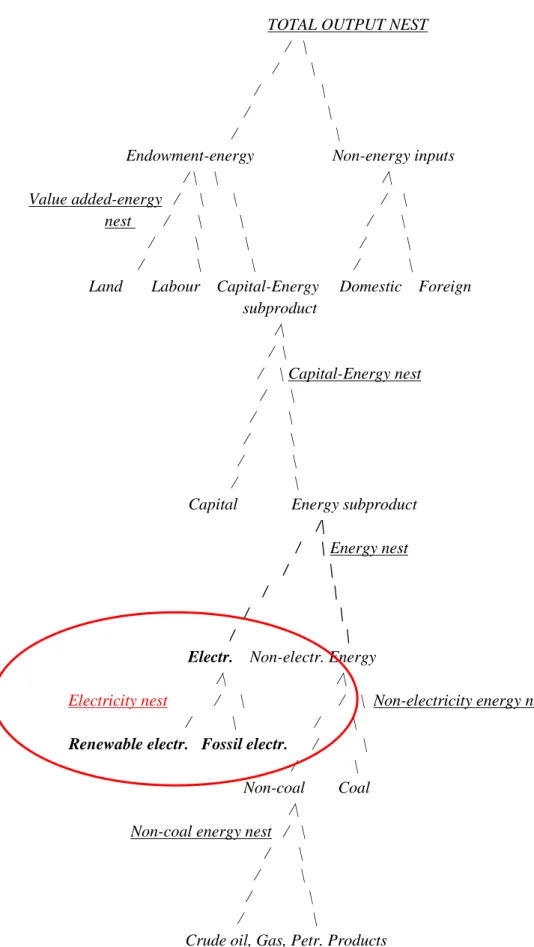
In GDyn-E ITA, the production functions are specified via a series of nested Constant Elasticity of Substitution (CES) functions. Sectoral output is a function of technology, aggregate value added-energy composite, and other intermediate inputs. Value added is produced using primary factors, namely land, labour, natural resources, and a energy composite. At its turn, the capital-energy composite is produced by combining capital and capital-energy, having a limited possibility to substitute energy for capital (Golub, 2013; Antimiani et al., 2013). In a lower nest, electricity can be substituted with electrical energy, while in the next lower nest coal can be substituted with non-coal energy sources. The lowest layer of nesting accounts for the choice among the remaining energy commodities, namely oil, gas, and oil products.
Two different alternatives have been elaborated to model the use of renewable electricity, as shown in Figures 1 and 2. In particular, the first alternative, called ITA2, models an electricity nest, in which it is possible to substitute between electricity generated by renewables and electricity
1
GTAP 7 Data Base Documentation is available here https://www.gtap.agecon.purdue.edu/databases/v7/v7_doco.asp 2 GTAP 8 Data Base Documentation is available here https://www.gtap.agecon.purdue.edu/databases/v8/v8_doco.asp 3
For more detail, see GTAP 9 Data Base Documentation, available here
https://www.gtap.agecon.purdue.edu/databases/v9/v9_doco.asp. GTAP-Power satellite data are provided free of charge for the subscribers of GTAP 9 Data Base.
9
generated by fossil fuels. This nest alters the existing nested structure in the sense that it is not connected to another one, namely it does not exist any other nest below. By contrast, the second alternative, ITA3, enlarges an existing nest, where electricity could be substituted with non-electrical energy, and it includes in the nest the two types of electricity, generated by renewables and fossil fuels. This enlarged nest is connected to a lower one where different non-electrical energy sources can be substituted.
In both cases the substitution elasticity is set to 0.5, but this is certainly an area for further improvement. First, the elasticity could be differentiated by country and/or based on econometric estimates (Costantini and Paglialunga, 2014), improving the reliability and realism of scenario results. Second, in the modelling alternative ITA3, the elasticity could be differentiated according to the concerned couple of energy sources. In particular, this would imply setting the elasticity at a lower value between both types of electricity and non-electrical energy (namely, renewable electricity versus non-electrical energy, and fossil electricity versus non-electrical energy), and at a higher value between the two types of electricity (renewable electricity versus fossil electricity). This would create greater substitution possibilities between the two types of electricity. Such intervention could be relevant also for the lower nest for substitution among non-coal energy sources, which is as well a three-good nest. However, in both cases this seems more complicated since it would alter the CES structure of the production function. Finally, it is worth mentioning that a sensitivity analysis, exploring how the results from these two alternatives react to changes in the substitution elasticities, could provide useful insights.
No changes to the model code were done for modelling the use of renewable electricity by household and government sectors. These sectors could indeed already use the new type of electricity according to their existing consumption functions. Nevertheless, also in these cases a sensitivity analysis to the values of cross-price and own-price substitution elasticities could have interesting outputs.
10
Figure 1 – Nested structure of production function: alternative 1 (ITA2)
TOTAL OUTPUT NEST / \
/ \ / \ / \ / \
Endowment-energy Non-energy inputs / \ \ /\
Value added-energy / \ \ / \ nest / \ \ / \ / \ \ / \ / \ \ / \
Land Labour Capital-Energy Domestic Foreign subproduct /\ / \ / \ Capital-Energy nest / \ / \ / \ / \ / \
Capital Energy subproduct
/\ / \ Energy nest / \ / \ / \ / \ Electr. Non-electr. Energy
/\ /\
Electricity nest / \ / \ Non-electricity energy nest / \ / \
Renewable electr. Fossil electr. / \
/ \ Non-coal Coal
/\ Non-coal energy nest / \
/ \ / \ / \ / \
11
Figure 2 – Nested structure of production function: alternative 2 (ITA3)
TOTAL OUTPUT NEST / \
/ \ / \ / \ / \
Endowment-energy Non-energy inputs / \ \ /\
Value added-energy / \ \ / \ nest / \ \ / \ / \ \ / \ / \ \ / \
Land Labour Capital-Energy Domestic Foreign subproduct /\ / \ / \ Capital-Energy nest / \ / \ / \ / \ / \
Capital Energy subproduct
//\ / / \ Energy nest / / \ / / \ / / \ / / \ / / \
Renewable electr Fossil electr. Non-electr. Energy
/\ Non-electricity energy nest / \ / \ / \ / \ Non-coal energy Coal
/\ Non-coal energy nest / \
/ \ / \ / \ / \
12
In the current analysis, a relatively low disaggregation level has been chosen, the main objective being not the detailed analysis of country results but the assessment of different modelling options (Table 1). The disaggregation just described is called Gdyn-E Ren.
It is important to highlight that Gdyn-E Ren corresponds, to our knowledge, also to the first experience in aggregating the GTAP-Power data to build a version of Gdyn-E model.
Table 1 – Countries included in Gdyn-E Ren
Name
Country/Countries
1. ITA Italy 2. FRA France 3. DEU Germany 4. GBR United Kingdom 5. ESP Spain6. REU Rest of Europe, including:
Austria, Belgium, Bulgaria, Cipro, Croatia, Czech Republic, Denmark, Estonia, Finland, Greece, Hungary, Latvia, Lithuania, Luxembourg, Malta, Netherlands, Norway, Poland, Portugal, Romania, Slovenia,
Slovakia, Sweden
7. USA United States
8. CHN China
9. IND India
10. ROW Resto of the world, including:
Albania, Argentina, Armenia, Australia, Azerbaijan, Bangladesh, Belarus, Benin, Bharain, Bolivia, Botswana, Brazil, Burkina Faso,
Cambodia, Cameroon, Canada, Caribbean, Central Africa, Chile, Colombia, Costa Rica, Cote d’Ivoire, Ecuador, Egypt, El Salvador, Ethiopia, Georgia, Ghana, Guatemala, Guinea, Honduras, Indonesia, Islamic Republic of Islamic, Israel, Japan, Kazakhstan, Kenya, Kuwait,
Kyrgyztan, Lao People’s Democratic Republic, Madagascar, Malawi, Malaysia, Mauritius, Mexico, Mongolia, Morocco, Mozambique, Namibia, Nepal, New Zealand, Nicaragua, Nigeria, Oman, Pakistan, Panama, Paraguay, Peru, Philippines, Qatar, Rest of Central America, Rest of East Asia, Rest of Eastern Africa, Rest of Eastern Europe, Rest of
EFTA, Rest of Europe, Rest of Former Soviet, Rest of North Africa, Rest of North America, Rest of Oceania, Rest of South African, Rest of South America, Rest of South Asia, Rest of Southeast Asia, Rest of the world,
Rest of Western Africa, Rest of Western Asia, Russia, Rwanda, Saudi Arabia, Senegal, Singapore, South Africa, South Central Africa, South
Korea, Sri Lanka, Switzerland, Taiwan, Tanzania, Thailand, Togo, Tunisia, Turkey, Uganda, Ukraine, United Arab Emirates, Uruguay,
13
At sectoral level, all electricity generated by RES has been aggregated in one sector, Renewable
electricity; also all base-load and peak-load fossil fuels for electricity generation have been
aggregated in another sector, Fossil electricity (Table 2).
Table 2 – Sectors included in Gdyn-E Ren
Name
Sector/sectors
1. AGR Agriculture, including:
Paddy rice; Wheat; Cereal grains nec; Vegetables, fruit, nuts Oil seeds; Sugar cane, sugar beet; Plant-based fibers
Crops nec; Bovine cattle, sheep and goats, horses; Animal products nec; Raw milk; Wool, silk-worm cocoons; fishing; forestry.
2. COAL Coal
3. GAS Natural gas
4. OIL Oil
5. OIL_PCTS Refinery
6. FOS_ELE Fossil electricity, including:
Nuclear power; Coal-fired power; Gas-fired power (base load); Oil-fired power (base load); Other power (base load); Gas-fired
power (peak load); Oil-fired power (peak load)
7. REN_ELE Renewable electricity, including:
Wind power; Hydroelectric power (base load); Hydroelectric power (peak load); Solar power
8. ELE_DISTR Electricity transmission and distribution
9. IRON_STEEL Iron and steel
10. CHEM_PETROC Chemical and petrolchemical
11. NON_FERMETAL Non-ferrous metals
12. NON_METMIN Non-metallic minerals
13. TRANSEQP Transport equipment, including:
Metal products; Motor vehicles and parts; Other transport equipment
14. MACHINERY Electronic and machinery equipment
15. OTH_MANUF Other manufacturing
16. FOOD_TOB Food and tobacco, including:
Bovine cattle, sheep and goat meat products; Meat products; Vegetable oils and fats; Dairy products; Processed rice; Sugar;
Beverages and tobacco products
17. PAPER Paper
18. WOOD Wood products
19. CONSTRUCT Construction
20. TEXTILE Textile, including:
Textiles; Wearing apparel; Leather products
21. LAND_TRASP Road transport
22. AIR_TRANS Air transport
23. WATER_TRANS Water transport
24. SERVICES Services, including:
Water; Trade; Communication; Financial services nec; Insurance; Business services nec; Recreational and other services; Public
14
GDyn-E Ren analyses the temporal horizon 2007-2030, in five intervals (2007-10; 2010-15; 2015-20; 2020-25;2025-30). The base year is 2007, so that simulation scenarios are comparable with those elaborated for the DDPP Country Report having the same base year. GTAP 9 Data Base offers the possibility to choose between 2007 and 2011 as base year, but for this exercise 2007 was preferred due to the reason explained above.
3 Simulation results
Baseline and policy scenarios will be described very briefly, since they were instrumental to validate two options for modelling renewable electricity. Moreover, further details can be found in the DDPP Country Report.
Baseline scenario was built basing on population, GDP and employment projections provided by relevant international institutions, such as European Commission, International Monetary Fund and International Labour Organization. Three different policy scenarios were elaborated with Times-Italy model, reducing emissions at 2050 by 80% relative to 1990 levels, and then transferred in CGE models GDyn-E and ICES. Each of them was based on different assumptions on technology penetration, in particular relative to energy efficiency, renewable energy sources and CCS (Carbon Capture and Storage).
In this exercise two policy scenarios will be taken into account:
Energy Efficiency (EFF), characterised by very high availability of energy efficiency technologies and relatively good penetration of RES for electricity generation and CCS technologies;
Demand Reduction (RED), characterised by a contraction of industrial production due to lower availability of energy efficiency and CCS technologies, and lower penetration of RES for electricity generation.
In DDPP Country Report several assumptions needed to be made for modelling a key issue such as renewable electricity in GDyn-E. Indeed, RES were not explicitly modelled, as no data on renewable electricity production or consumption were included in the model. Nevertheless, in GDyn-E ITA, RES were implicitly taken into account by combining three main approaches. First, a carbon tax revenue recycling scheme had been introduced to finance R&D in the electricity sector. R&D increases output-augmenting technical change in the electricity sector, which as a consequence would need less fossil fuels in power generation. Second, in the electricity sector the
15
elasticity of substitution between capital and energy has been increased, in order to model wind and solar, which are the prevailing capital-intensive RES for power production. Third, in all sectors the substitution elasticity between electrical and non-electrical energy has been increased, to foster the use of electricity, which due to the two previous interventions is less carbon-intensive and more capital-intensive.
ITA version of the model, including these features, will be compared with the versions ITA2 and ITA3 including electricity generated by RES and explicitly modelling its consumption by key economic sectors. In particular, the results provided by policy scenarios EFF and RED in the three versions will be analysed, focusing on specific variables. The following paragraphs will analyse the trends of different key variables: primary and final energy consumption (Table 3 and 4), carbon taxes associated to emission reduction (Figure 3), GDP impacts (Figure 4 and Table 5), employment (Figure 5), and international trade (Figure 6 and 7).
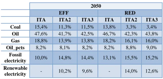
Table 3 shows the share in primary consumption corresponding to each energy source in the two policy scenarios. In general, ITA3 alternative is characterised by a slightly higher use of oil and oil products and a lower use of renewable electricity relative to ITA2, reflecting the substitution structure in the nest. It is interesting to note how the availability of renewable electricity diversifies the primary consumption mix between EFF and RED scenarios, with a higher contraction of coal in the second one.
Table 3 – Primary consumption (% on the total)
2050
EFF RED
ITA ITA2 ITA3 ITA ITA2 ITA3
Coal 15,4% 11,3% 11,5% 13,8% 3,3% 3,4% Oil 47,6% 41,7% 42,5% 46,7% 42,3% 43,8% Gas 18,8% 13,9% 13,8% 18,2% 16,1% 16,0% Oil_pcts 8,2% 8,1% 8,2% 8,2% 8,8% 9,0% Fossil electricity 10,0% 14,8% 14,4% 13,1% 15,5% 15,2% Renewable electricity - 10,2% 9,6% - 14,0% 12,6%
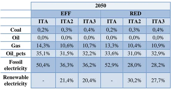
Table 4 shows the final consumption mix under the three versions. The difference between ITA and ITA2-ITA3 versions are more pronounced for gas, which is higher in ITA. The pattern already described for oil products and renewable electricity is observed also in this case. This shows how the nested structure influences both primary consumption and final energy consumption.
16
Table 4 – Final consumption (% on the total)
2050
EFF RED
ITA ITA2 ITA3 ITA ITA2 ITA3
Coal 0,2% 0,3% 0,4% 0,2% 0,3% 0,4% Oil 0,0% 0,0% 0,0% 0,0% 0,0% 0,0% Gas 14,3% 10,6% 10,7% 13,3% 10,4% 10,9% Oil_pcts 35,1% 31,5% 32,2% 33,6% 31,0% 32,9% Fossil electricity 50,4% 36,3% 36,2% 52,9% 28,0% 28,2% Renewable electricity - 21,4% 20,4% - 30,2% 27,7%
The policy objective in terms of CO2 emissions, which in all scenarios decrease by more 70%
relative to the baseline, entails a reduction in energy consumption. It is interesting to look at the trend followed by the marginal cost of emission reduction, which is computed by the model as carbon tax (Figure 3). It could be surprising to note that carbon tax is lower in ITA2 and ITA3, but this could be due to the fact that these two versions are characterised by a lower electricity carbon content. Indeed, including renewable electricity in the data lowers the overall carbon content of power generation. Then, if the starting point is more “carbon efficient”, the marginal cost of increasing this efficiency – namely, reducing emissions – could be higher. However, further investigation is needed relatively to this issue4.
4 A very simple sensitivity analyisis has been performed, showing that increasing the substitution elasticity in the new nests in both ITA2 and ITA3 would lower the carbon tax values in the observed period.
17
Figure 3 – Implicit carbon taxes in policy scenarios (2015=1)
Figure 6 compares the cumulated GDP growth rate in policy scenarios as difference relative to the baseline, showing how the impacts are always more important in ITA version of the model, where renewable electricity is not modelled. The gap between ITA and ITA2-ITA3 versions is particularly relevant in EFF scenario. ITA3 version, with the nest modelling substitution among renewable electricity, fossil electricity and non-electrical energy, is associated to the most limited GDP impacts, both in RED and EFF scenario.
0 10 20 30 40 50 60 70 2015 2020 2025 2030 2035 2040 2045 2050
EFF ITA EFF ITA2 EFF ITA3
18
Figure 4 – Cumulated GDP growth rate in baseline and policy scenarios
The information on GDP can be looked in another perspective, namely in terms of average annual growth rate (Table 5). Also in this case, the results show that ITA2 and ITA3 versions are associated to better GDP trends. Consistently with Figure 4, ITA3 provides the highest growth rates. This could be due to the wider extent of substitution possibilities which enables the economy to adapt better to the decarbonisation objective.
Table 5 – GDP average annual growth rates
2010-2020 2020-2030 2030-2040 2040-2050 2010-2030 2010-2050 EFF ITA 0.31 1.42 1.23 0.68 0.86 0.91 EFF ITA2 0.27 1.45 1.34 0.98 0.86 1.01 EFF ITA3 0.28 1.46 1.36 1.02 0.87 1.03 RED ITA 0.31 1.38 1.07 0.53 0.84 0.82 RED ITA2 0.28 1.42 1.12 0.42 0.85 0.81 RED ITA3 0.28 1.42 1.16 0.50 0.85 0.84
Another relevant dimension to look at when evaluating economic impacts is sectoral value added5. ITA2 and ITA3 versions are associated to mitigated negative impacts and better positive impacts, in both scenarios. The new versions of GDyn-E maintan the differentiation in results observed in two policy scenarios, with RED scenario having stronger negative impacts.
5
The focus in all the following figures will be on industrial sectors, excluding agriculture and services. -14% -12% -10% -8% -6% -4% -2% 0% 2% 2010 2015 2020 2025 2030 2035 2040 2045 2050
EFF ITA EFF ITA2 EFF ITA3
19
The high positive impacts observed in iron and steel and non-ferrous metals sectors are consistent with the results from ICES model in DDPP Country Report. Renewable electricity was included in ICES, differently from the GDyn-E version used in the DDPP Report, and the model showed a strong value added increase in energy intensive sectors. This could be due to the fact that these industries provide raw materials, metals, and inputs for a low-carbon economy and in particular for renewable electricity development. Deep reductions are observed in the construction sector in ITA2 and ITA3 versions, and such behaviour would deserve further investigation.
Figure 5 – Impacts on value added (difference relative to the baseline)
GDyn-E model assumes full employment, so after the policy interventions labour force would not increase or decrease in absolute terms but only be reallocated among sectors. It is worth mentioning
-30% -20% -10% 0% 10% 20% 30% 40% Foo d a n d t o b acco Iro n a n d s te el Che m ic al an d p etro ch e m ic al N on f errou s m e tal s N o n m eta llic m in e ra ls Me ta lli c p ro d u cts Tra n sp o rt eq u ip m e n t Ma ch in e ry Ot h er m an u fact u rin g Pa p er p ro d u cts Con stru ctio n Te xt ile
EFF ITA EFF ITA2 EFF ITA3
-60% -50% -40% -30% -20% -10% 0% 10% 20% 30% 40% Foo d a n d t o b acco Iro n a n d s te el Che m ic al an d p etro ch e m ic al N on f errou s m e tal s N o n m eta llic m in e ra ls Me ta lli c p ro d u cts Tra n sp o rt eq u ip m e n t Ma ch in e ry Ot h er m an u fact u rin g Pa p er p ro d u cts Con stru ctio n Te xt ile
20
that the deep decarbonisation process would induce a significant downsizing of fossil-fuel-related sectors including extraction, refining, and commercialisation, and thus employment would reallocate among the other sectors. In the following, the employment impacts will be commented referring to skilled labour force. Impacts on unskilled labour force are analogous in the direction of the change, and also similar in terms of percentage variation.
In RED scenario, less technological options are available to meet the decarbonisation target and then the contraction of energy use is higher. Due to these reasons, the employment effects are generally more important in absolute value.
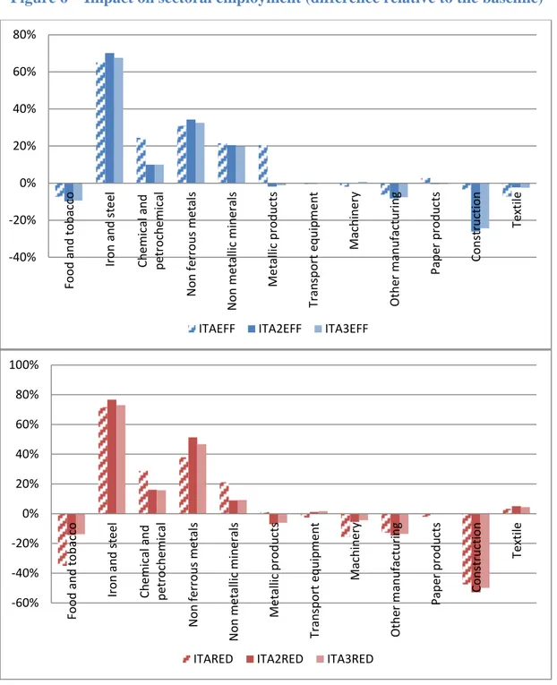
In both scenarios, modelling renewable electricity in ITA2 and ITA3 versions generally implies better impacts. As already said for value added impacts, also in this case the positive impacts observed in energy intensive industries are consistent with results from ICES model. The availability of renewable electricity does not entail an improvement of negative impacts in the few sectors where they are observed.
21
Figure 6 – Impact on sectoral employment (difference relative to the baseline)
Figure 6, 7 and 8 analyse the impacts on trade balance. Looking at exports, an increase is observed in almost all industrial sectors. Results from the alternative versions ITA2 and ITA3 are consistent with ITA version for both scenarios. In ITA2 and ITA3 a higher increase is observed in iron and steel and non-ferrous metals sectors, and to a lesser extent in chemical and petrochemical sector.
-40% -20% 0% 20% 40% 60% 80% Food a n d t ob acco Iro n a n d s te el Che m ic al an d p etro ch e m ic al N o n f erro u s me tal s N o n m eta llic m in e ra ls Me ta lli c p ro d u cts Tra n sp o rt eq u ip m e n t Ma ch in e ry Ot h er m an u fact u rin g Pa p er p ro d u cts Con stru ctio n Te xt ile
ITAEFF ITA2EFF ITA3EFF
-60% -40% -20% 0% 20% 40% 60% 80% 100% Foo d a n d t o b acco Iro n a n d s te el Che m ic al an d p etro ch e m ic al N o n f erro u s me tal s N o n m eta llic m in e ra ls Me ta lli c p ro d u cts Tra n sp o rt eq u ip m e n t Ma ch in e ry Ot h er m an u fact u rin g Pa p er p ro d u cts Con stru ctio n Te xt ile
22
Figure 7 – Impact on exports (difference relative to the baseline)
As for imports, lower reductions are observed in EFF scenario. It is interesting to note that imports of iron and steel and non-ferrous metals decrease in ITA version and increase in ITA2 and ITA3. This pattern could be due to the increase in domestic demand of these goods as relevant inputs for renewable energy development. In RED scenario, instead, ITA2 and ITA3 versions are associated to higher reductions in almost half of the sectors. This is probably due to the higher GDP reduction and the associated contraction in demand, both as intermediate industrial use and as final use. Also in RED scenario, an increase in imports is observed in iron and steel and non-ferrous metals sectors, likely associated to higher domestic demand in ITA2 and ITA3.
-40% -20% 0% 20% 40% 60% 80% Food a n d t ob acco Iro n a n d s te el Che m ic al an d p etro ch e m ic al N o n f erro u s me tal s N o n m eta llic m in e ra ls Me ta lli c p ro d u cts Tra n sp o rt eq u ip m e n t Ma ch in e ry Ot h er m an u fact u rin g Pa p er p ro d u cts Con stru ctio n Te xt ile
ITAEFF ITA2EFF ITA3EFF
-20% 0% 20% 40% 60% 80% 100% 120% 140% 160% Foo d a n d t o b acco Iro n a n d s te el Che m ic al an d p etro ch e m ic al N o n f erro u s me tal s N o n m eta llic m in e ra ls Me ta lli c p ro d u cts Tra n sp o rt eq u ip m e n t Ma ch in e ry Ot h er m an u fact u rin g Pa p er p ro d u cts Con stru ctio n Te xt ile
23
Figure 8 – Impact on imports (difference relative to the baseline)
It is important to look also at energy imports and the effects of decarbonisation policies on energy dependency. Results from ITA2 and ITA3 versions are in line with ITA, with imports decreasing more in the new versions. Divergent results are observed for coal, for which under EFF scenario imports decrease slightly less in ITA2 and ITA3 than in ITA, and much more in RED scenario. The difference in EFF scenario could be too small to be relevant, whereas the higher decrease in RED scenario could be due to the fact that coal is the more carbon intensive generation source, and thus it is the one more deeply reduced once generation from renewables is considered.
-50% -40% -30% -20% -10% 0% 10% 20% Food a n d t ob acco Iro n a n d s te el Che m ic al an d p etro ch e m ic al N o n f erro u s me tal s N o n m eta llic m in e ra ls Me ta lli c p ro d u cts Tra n sp o rt eq u ip m e n t Ma ch in e ry Ot h er m an u fact u rin g Pa p er p ro d u cts Con stru ctio n Te xt ile
ITAEFF ITA2EFF ITA4EFF
-60% -50% -40% -30% -20% -10% 0% 10% 20% Food a n d t ob acco Iro n a n d s te el Che m ic al an d p etro ch e m ic al N o n f erro u s me tal s N o n m eta llic m in e ra ls Me ta lli c p ro d u cts Tra n sp o rt eq u ip m e n t Ma ch in e ry Ot h er m an u fact u rin g Pa p er p ro d u cts Con stru ctio n Te xt ile
24
Figure 9 – Impact on energy imports (difference relative to the baseline)
Figures 12 and 13 provide a synthesis graph for each policy scenario in order to help in summarising the differences among different versions. In each graph, policy impacts in 2050 are shown as percentage changes relatively to the baseline scenario. Since the results are similar in most cases between ITA2 and ITA3 versions, in both figures only ITA2 is shown. The tables with the corresponding data, as well as the data for ITA3, are available in the Annex (Table 1 and Table 2).
Figure 10 – Policy scenario impacts on selected variables: EFF
-100% -80% -60% -40% -20% 0% Coa l Oil Gas
ITAEFF ITA2EFF ITA4EFF ITARED ITA2RED ITA4RED
-75% -50% -25% 0% 25% GIC TFC Energy intensity Carbon intensity Energy dependency GDP VA Employment Import Export
25
Starting with EFF scenario, the reduction in Gross Inland Consumption (GIC) and Total Final Consumption (TFC) is almost the same in the two versions. The reduction in energy intensity is slightly higher in ITA version, consistently with the fact that no renewable electricity is available and GDP impacts are higher. Carbon intensity reduction is higher in ITA2 and ITA3 versions, reflecting the availability of renewable electricity. Energy dependency decreases a little less in ITA model, as already shown by data in Figure 9. The different impact on energy dependency shows how the effects of including renewable electricity influences the countries performance in reaching energy policy objectives, at the same time confirming one of the multiple benefits of energy efficiency (IEA, 2014). In terms of macroeconomic variables the differences are more important. GDP impacts are higher in ITA model, as well as impacts on value added, total employment and total imports. As for total exports, the positive impacts are higher in ITA than in ITA2 model. In RED scenario the policy impacts are more in line among the two versions, as shown in Figure 11.
Figure 11 – Policy scenario impacts on selected variables: RED
4 Conclusions
This work is aimed at documenting the first attempts in building up a new version of GDyn-E ITA model including renewable electricity. Two alternative versions have been tested referring to existing policy scenarios developed for DDPP in which ENEA was involved. In particular, the two options explored differ in the industrial production function, and specifically relative to the nest using electricity from renewable sources.
-75% -50% -25% 0% 25% 50% GIC TFC Energy intensity CO2 emissions Energy dependency GDP VA Employment Import Export
26
In both cases, the results of the new version of GDyn-E ITA model seem robust. Since the main objective was validating two new versions, obtaining results aligned with the existing version is a good result, when no difference was expected or directly explainable. No preferred option has been identified in the current work, and the fact that both the alternatives seem robust could allow the researcher to choose the more suited option for the specific research question. For example, if the focus is an analysis of electricity market, ITA2 could be well-suited, improved with a better detail of base-load and peak-load generation sources.
Relatively to interventions to improve GDyn-E model identified in previous works (Martini, 2016), introducing an explicit consideration of renewable energy seems a relevant step in improving the quality and information associated to the simulation scenarios.
Clearly, the approach could be further improved. As already mentioned, the disaggregation of base-load and peak-base-load generation sources, as offered in GTAP-Power satellite data, could be an example of possible improvements of the current versions. During these days, a new version of the GTAP-E model based on GTAP-Power database has been presented at the Annual GTAP Conference (Peters, 2016). In the future, a comparison of the two alternatives presented in this work with this new version could inspire further improvements and help in choosing a preferred modelling option for the nest.
Further interventions, such as developing sensitivity analysis and performing a decomposition analysis of model results, could still contribute to fully exploit the model potential and to strengthen the reliability of its output.
27
References
Antimiani A.,Costantini V., Martini C., Palma A. Tommasino, M. C. (2013), “The GTAP-E: Model Description and Improvements”, in The Dynamics of Environmental and Economic Systems. Innovation, Environmental - - Policy and Competitiveness. (Eds) Costantini V. and Mazzanti, pp. 3-24. Springer Book, Netherlands.
Burniaux, J.-M., Truong, T.P., (2002), “GTAP-E an energy-environmental version of the GTAP model”, GTAP Technical Papers, No. 16. Center for Global Trade Analysis, Purdue University, West Lafayette, Indiana, USA 47907-1145.
Costantini, V., and Paglialunga, E. (2014) “Elasticity of substitution in capital-energy relationships: how central is a sector-based panel estimation approach?”, SEEDS Working Paper Series, 13/2014. Gaeta, M. and Baldissara, B. (2011), “Il modello energetico Times-Italia. struttura e dati versione 2010”, ENEA-RT-2011-09, http://opac22.bologna.enea.it/RT/2011/2011_9_ENEA.pdf
Golub, A. (2013), “Analysis of climate policies with GDyn-E”, GTAP Technical Paper 4292, Center for Global Trade Analysis, Department of Agricultural Economics, Purdue University,
https://www.gtap.agecon.purdue.edu/resources/download/6632.pdf
Hertel, T.W. (1997), “Global Trade Analysis: Modeling and applications”, Cambridge University Press, Cambridge, https://www.gtap.agecon.purdue.edu/products/gtap_book.asp
Ianchovichina, E.,McDougall, R. (2001), “Theoretical Structure of Dynamic GTAP”, GTAP Technical Paper No. 17, Center for Global Trade Analysis, Department of Agricultural Economics, Purdue University, https://www.gtap.agecon.purdue.edu/resources/res_display.asp?RecordID=480
Markandya, A., Antimiani A., Costantini V., Martini C., Palma, A., Tommasino M.C. (2015), “Analyzing Trade-offs in International Climate Policy Options: The Case of the Green Climate Fund”, World Development, 74, 93–107.
Martini, C. (2016) “A Macroeconomic evaluation of energy efficiency objectives using GDyn-E ita model”, ENEA-RT-2016-02, http://openarchive.enea.it/bitstream/handle/10840/7376/RT-2016-02-ENEA.pdf?sequence=1
Martini, C. and Tommasino, M.C. (2011), “GTAP-DYN drivers for the EFDA-TIMES Model”, Final Report EFDA Reference: WP 10-SER-ETM-7, https://www.euro-fusion.org/wpcms/wp-content/uploads/2014/12/WP10-SER-ETM-7.pdf
28
Martini, C. and Tommasino, M.C. (2010) “General equilibrium modelling for energy policies evaluation: the GTAP-E ITA model”, ENEA-RT-2010-10,
http://opac22.bologna.enea.it/RT/2010/2010_10_ENEA.pdf.
Narayanan, G., B., Aguiar A., and McDougall, R. (2012), “Global Trade, Assistance, and Production: The GTAP 8 Data Base”, Center for Global Trade Analysis, Purdue University,
https://www.gtap.agecon.purdue.edu/databases/v8/v8_doco.asp
Narayanan, B., Dimaran, B., McDougall, R. (2012), “GTAP 8 Data Base Documentation - Chapter
2: Guide to the GTAP Data Base”,
https://www.gtap.agecon.purdue.edu/resources/res_display.asp?RecordID=3777
Peters, J. C. (2015), “The GTAP-Power Data Base: Disaggregating the Electricity Sector in the GTAP Data Base”, Journal of Global Economic Analysis, 1, 209-250.
Peters, J. C. (2016), “GTAP-E-Power: An electricity-detailed extension of the GTAP-E model”, GTAP 2016 Conference Paper, GTAP Resource #4891,
https://www.gtap.agecon.purdue.edu/resources/res_display.asp?RecordID=4891
Truong, P. T. and Lee, H.-L. (2003), “GTAP-E Model and the ‘new’ CO2 Emissions Data in the GTAP/EPA Integrated Data Base – Some Comparative Results”, GTAP Resource #1296, Center for
Global Trade Analysis, Purdue University,
https://www.gtap.agecon.purdue.edu/resources/res_display.asp?RecordID=1296
Virdis, M. R., Alloisio, I., Borghesi, S., De Cian, E., Gaeta, M., Martini, C., Parrado, R., Tommasino, M. C., Verdolini, E. (2015), “Pathways to Deep Decarbonisation in Italy”,
http://deepdecarbonization.org/countries/#italy
Walmsley, T. L., Anguiar, A.H., Narayanan B. (2012), “Introduction to the Global Trade Analysis Project and the GTAP Data Base”, GTAP Working Paper No. 67, Center for Global Trade
Analysis, Purdue University,
29
Annex
Table A1 - Policy scenario impacts on selected variables: EFF
2050 ITA wrt Baseline 2050 ITA2 wrt Baseline 2050 ITA4 wrt Baseline GIC -65,9% -59,7% -60,1% TFC -49,3% -44,2% -45,2% Energy intensity -57,5% -53,5% -54,5% Carbon intensity -64,6% -67,3% -67,7% Energy dependency -2,5% -4,0% -4,0% GDP -9,7% -4,0% -4,7% VA -19,7% -13,2% -12,2% Employment -12,7% -9,2% -8,4% Import -21,9% -12,4% -11,6% Export 16,9% 11,4% 10,9%
Table A2 – Policy scenario impacts on selected variables: RED
2050 ITA wrt Baseline 2050 ITA2 wrt Baseline 2050 ITA4 wrt Baseline GIC -70,2% -69,3% -70,0% TFC -56,9% -54,8% -56,8% Energy intensity -60,9% -58,4% -60,2% CO2 emissions -70,6% -72,8% -73,1% Energy dependency -2,5% -3,6% -3,7% GDP -12,8% -10,9% -12,0% VA -23,7% -26,2% -24,5% Employment -15,6% -19,2% -17,9% Import -26,2% -25,8% -24,2% Export 21,0% 31,4% 29,5%
ENEA
Servizio Promozione e Comunicazione
www.enea.it
Stampa: Laboratorio Tecnografico ENEA - C.R. Frascati giugno 2016