Corso di Dottorato in Fisica Applicata
(XVIII Ciclo)
Tesi di Dottorato
Nonlinear collisionless plasma dynamics
Laura Galeotti
January 2006
Relatore:
Introduction 3
1 Collisionless plasma phenomena 11
1.1 Kinetic theory of small amplitude plasma waves in a field free
colli-sionless plasma . . . 11
1.2 Landau damping . . . 15
1.2.1 Linear regime . . . 15
1.2.2 Electron trapping and O’Neil regime . . . 19
1.2.3 Long time evolution of Landau damping . . . 23
1.3 Plasma wave echoes . . . 24
1.4 Two stream instability . . . 31
1.4.1 Ion-acoustic waves . . . 34
1.5 Correlations . . . 36
2 Numerical schemes 42 2.1 The splitting scheme . . . 42
2.2 Van Leer interpolation scheme . . . 46
2.3 Spline interpolation scheme . . . 49
3 Numerical results 51 3.1 Asymptotic evolution of non-linear Landau damping . . . 52
3.2 Non linear regime of two stream instability . . . 59
3.3 The echo benchmark . . . 67
3.4 Correlations . . . 74
3.5 Conclusions . . . 84
A Bernstein-Greene-Kruskal (BGK) waves 86
B Analytical detailed computation of an echo 91
C Propagation of waves in a hot uniformly magnetized plasma 95 C.1 Harris pinch . . . 104
D Numerical electromagnetic results 108
D.1 Propagation of finite amplitude electromagnetic perturbations in a ho-mogeneous magnetized collisionless plasma . . . 109 D.2 Propagation of finite amplitude electromagnetic perturbations in a
in-homogeneous magnetized collisionless plasma . . . 112
In high temperature laboratory and rarefied space plasmas, many situations arise where the observed dynamics is characterized by non collisionality. This is due to the fact that, in such plasmas, the collision frequency can be orders of magnitude smaller than the typical frequencies of the plasma dynamics (as the plasma frequency), corresponding to a mean free path of the particles much longer than all other plasma characteristic length scales. From a theoretical point of view, the dynamics of these plasmas can be considered as Hamiltonian.
The study of such non collisional systems represents one of the widest fields of investigation of plasma physics. The capability of generating, during the time evolu-tion, smaller and smaller scales in the velocity space is a characteristic of the majority of the processes developing in such plasmas. Thanks to this feature, it is possible to observe fascinating phenomena, like the Landau damping, in which the passage of en-ergy through macroscopic to microscopic scales can produce the exponential damping of macroscopic oscillating quantities as the electric field and the charge density. In this process the initial energy associated to these macroscopic quantities is not dis-sipated, since the system is collisionless, but, it is stored in the distribution function as velocity-space fluctuations that oscillate indefinitely in time on increasingly finer velocity scales (the so-called ballistic term). This interplay between macroscopic and microscopic processes is very elegantly exemplified by the plasma wave echoes [1, 2]. Echoes are, in fact, one of the most direct proofs and one of the more significant demonstration of microscopic reversibility in collisionless plasmas since, as a matter of fact, they are capable to bringing back on macroscopic scales the memory of the initial perturbation Landau damped away in time.
Like in the Landau damping and in the echo phenomenon, the dynamics of a collisionless system, especially in the long time, non linear evolution, is often driven by kinetic effects. Therefore, to describe theoretically its evolution, a kinetic approach is
necessary. This kinetic theory is a mean field theory, in which Coulomb interactions between particles are replaced by a common mean electromagnetic field. In other words, each particle feels the averaged field of the collective system, while single particle interactions are neglected. The equation which governs the evolution of such systems is known as the Vlasov equation.
This equation, self-consistently coupled with Maxwell ones, describes the plasma dynamics for times shorter than the binary collision time in terms of the distribution function of particles f (x, v, t). The distribution function represents the number of particles per unit volume, at the time t, in the point (x, v) of the phase space. One of the fundamental characteristics of the Vlasov equation is that different curves of level of the distribution function in the phase space can wind round themselves in very complicate ways but cannot reconnect. Furthermore this equation is characterized by the fact that any function G(f ) is a constant of motion, i.e. dG/dt = 0, as, in partic-ular, the n-order invariants In=
R
fndxdv. Through Vlasov and Maxwell equations,
the distribution function time evolution is calculated self-consistently with the elec-tromagnetic fields produced by the plasma particles. However, the Vlasov-Maxwell system is a non linear system of equations, and hence to solve it analytically, even in simplified problems, results usually very difficult and in general even impossible. For this reason, when one wants to study the non linear dynamics of a plasma, numerical simulations are one of the most effective tools of investigation. However, the necessity of the numerical approach to discretize the equations on a numerical mesh introduces a strong limit. In fact, in Vlasov simulations, when a process develops scales so small to be comparable with the size of the numerical mesh, the algorithm becomes neces-sarily unable to describe correctly the plasma dynamics, with the consequent effect of introducing in the system numerical dissipation and dispersion. The role of these numerical dissipative effects on the study of collisionless plasma dynamics is a com-plex question still open and can be considered as one of the outstanding problems of plasma physics. One of the main problems to understand is how much the feedback of small scales on large ones is relevant for the macroscopic dynamics, even if the mesh length scale, that is comparable to the dissipative one, is much shorter than any physical length scale.
We tried to face this question by considering several specific cases of one dimen-sional electrostatic collisionless dynamics and, we made numerical simulations of the
non linear long time evolution of several non collisional plasma systems by varying the mesh size and/or the algorithm used to solve the Vlasov equation.
The first phenomenon investigated is the long time evolution of the Landau damp-ing phenomenon which can be summarized as a resonant interaction between a plasma wave and particles moving at nearly its phase velocity. The effect of this interaction is an exchange of energy between these particles and the wave. In the case in which the initial distribution function is Maxwellian and the wave has a positive phase velocity, the net transfer of energy is from the wave to the particles, producing the damp-ing of the wave in time. However, durdamp-ing the non-collisional dampdamp-ing process, other mechanisms can come into play changing the evolution of the phenomenon. When the amplitude of the initial wave is ”sufficiently” large, one of these mechanisms is represented by the particles trapping in the potential well of the wave. This process has a characteristic time τp, called the trapping time, that is the time necessary for
a particle to go across the potential well and bounce back. Hence, the long time dynamics of the plasma can change in conformity with the relations between the characteristic times scales of the system (Landau damping time τL, trapping time τp
and the wave oscillation period τ0 = 1/ω). When τp À τL À τ0 (Landau regime)
the plasma oscillation for large times is exponentially damped to zero [3], while when
τL À τp À τ0 particles are rapidly trapped before the wave is damped and, at t
about τp, the linear Landau theory breaks down. The result is that, at large times,
the wave amplitude reaches a constant nonzero value (O’Neil regime) [4]. If instead
τp is about τL, the behaviour of the system is intermediate [5]. In the case when
par-ticle trapping is relevant in the system dynamics, phase space vortices, representing particle oscillations in the potential wells, are generated. We are interested in the regime in which vortices are created because it represents one of the most important and typical examples of the violation of the Vlasov equation.
Our numerical study of the long time evolution of Landau damping has been made in the regime in which τL ' τp with the initial perturbation amplitude such
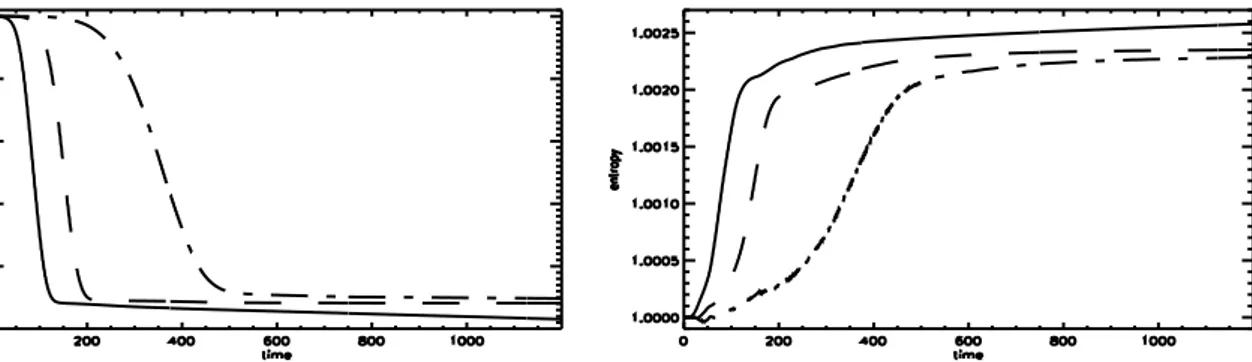
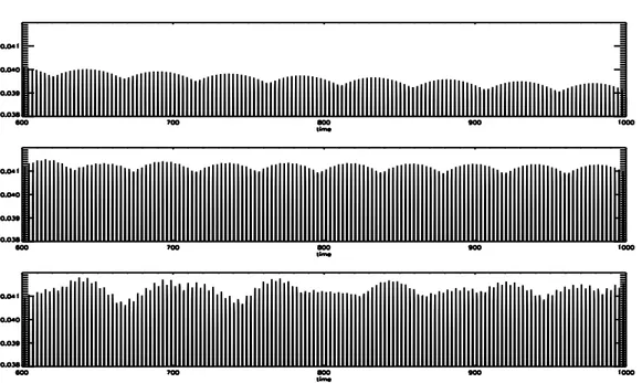
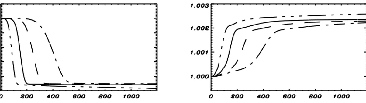
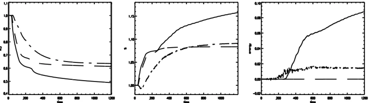
that a phase space vortex is generated around the resonant velocity. In our model we take the protons as a fixed neutralizing background since the dynamics under study evolves on the electron time scale. We compared the results obtained with different meshes and three different numerical schemes, corresponding to different values of artificial numerical dissipation. Through the measure of macroscopic quantities (the
distribution and number of trapped particles, invariants, electric field, etc...), we found that, at large times, the same initial plasma system reaches different final macroscopic states depending on the grid size and/or the numerical scheme. These final states are a superposition of ’averaged’ Bernstein-Greene-Kruskal (BGK) states [6, 7], i.e. a superposition of exact solutions of Vlasov-Poisson equations, stationary in the reference frame moving at the phase velocity of the wave, obtained averaging the particle distribution function of these states over the energy curves.
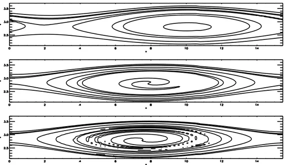
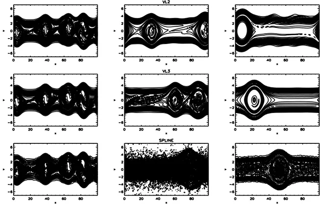
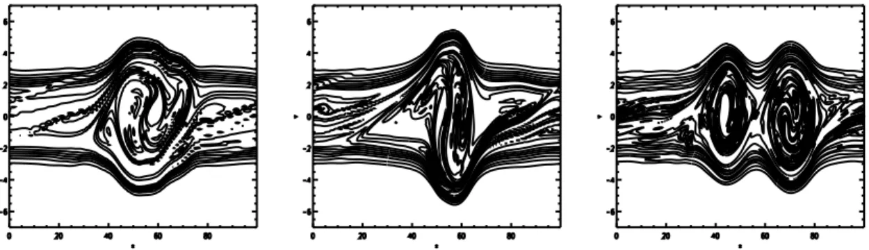
Differences among final macroscopic states of the Vlasov Poisson system are even more evident in the results of the two stream instability evolution, an instability which develops thanks to the initial anisotropy in velocity of the particle distribution function given by two counter streaming beams carrying no net total current in the system. The study of its linear and non-linear behaviour [8] has acquired new inter-est in the last ten years with the discovery of bipolar electric field pulses in space plasmas (Earth’s ionosphere [9, 10], magnetosphere [11] and foreshock region [12]). We are interested in this process because it produces a vortex that involves the bulk of the distribution function and not only a small portion as in the non linear Lan-dau damping. We investigated the evolution of this instability for a one dimensional unmagnetized collisionless plasma with an initial equilibrium configuration where the electrons are distributed in two beams with equal but opposite mean velocities, while (as a first step) protons are considered of infinite mass. When the system is per-turbed, the amplitude of the electric perturbation increases to the disadvantage of electrons kinetic energy, until it becomes large enough to trap electrons starting from less energetic ones. At this point the instability begins to saturate and a new sta-ble state is reached. In the phase space, the oscillations of the trapped electrons in the potential well are represented by vortices. The number of vortices which can be generated by this system depends on the spatial dimension Lx of the phase space.
If more vortices are generated in the system, they interact together [13, 14]. This interaction process of merging (inverse cascade) is forbidden in the Vlasov collisionless theory and is driven by the artificial dissipation introduced by the numerical approach. We observed that varying the length scale of the numerical grid, corresponding so to vary the artificial dissipative effects, changes both the way in which the vortices interact together to develop a final unique vortex and the characteristic time in which this merging process is completed.
The cause of the differences among final states of the Vlasov-Poisson system is hence due to the fact that simulations made with different algorithms or with the same algorithm but with different resolution grids, brings in the system different quantities of artificial effects which are relevant also for the macroscopic dynamics, even if the dissipative length scale is much shorter than any physical length scale. Therefore, when artificial dissipation comes into play, even if we are formally dealing with a collisionless plasma, the final effect will be very similar to inserting in the system a collisional operator.
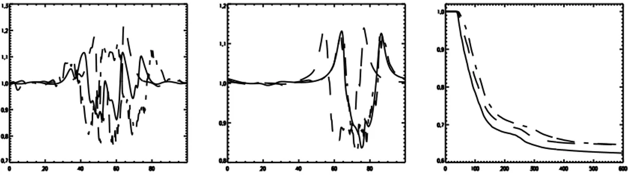
Since the echo phenomenon, for which a non linear solution is available, is one of the most sensitive process to ”collisions”, capable of distinguish between collisional or non-collisional damping effects, we have decided to employ it for the study of numerical schemes to investigate the dissipative effects problem. But how the echo manage to realize the differences between a collisionless and a collisional system? Let’s now give a brief explanation. A wave echo arises when two plasma waves are excited in the plasma with a time delay and, long after they have been Landau damped away, a macroscopic electric field reappears because of the nonlinear constructive interference between the ballistic terms of the two waves. In absence of dissipation, the memory of the two plasma waves, after they are Landau damped away exponentially, is stored in the ballistic terms. Instead, if collisions are present in the system, they can destroy the phase informations stored in these ballistic terms before the echo appears. A detailed analytical study of this phenomenon was developed by O’Neil [15] and showed how Coulomb collisions and microturbulence can affect the final amplitude and shape of the echo. This very fine sensibility of the echoes to dissipative effects, permits us to use this phenomenon to investigate the dissipative properties of a numerical code [16]. We tested, with the echo phenomenon, all the algorithms we used at different numerical resolutions. We found that code accuracy affects the final amplitude and shape of the echo in agreement with theoretical analysis. In the limit of very high resolution, no grids dissipative effects are introduced in the system at least for t < techo. The
echo test results more discriminating than those based on the conservation of (a finite set of) Casimir invariants (see Ref. [17]). In fact, in all runs where there is a decrease of the echo’s amplitude (up to complete disappearance) with respect to the expected value, due to any kind of (numerical) dissipative effect, the set of Casimir invariants of the Vlasov - Poisson system (here up to third order, m = 1, 2, 3) are
”perfectly” conserved (i.e. no variations are observed all along the simulation). Indeed such invariants, often considered as the relevant test for a Vlasov code, may provide misleading informations since they are global quantities unable to capture small-scale features of non-Vlasov local effects.
Considering all these results, one question arises: up to what point can a system, studied through numerical simulations, be considered as really non-collisional? As seen before, in fact, even if the plasma under study is formally collisionless, when the numerical scheme becomes unable to describe the system small scales, collisional effects come into play. A way to understand how and when the plasma looses its non collisionality is given by the study of particle correlations. As already mentioned, in a collisionless system, and therefore for the Vlasov theory, the correlations, as for example binary interactions, are negligible with respect to the averaged field produced by all the particles of the plasma. However, when strong spatial and velocity gradients are generated by the system during the dynamical evolution, correlations become more and more important at least in local large gradient regions. For this reason, we studied the generation of binary correlations in numerical simulations of two different kind of collisionless plasma systems: a one dimensional electrostatic two stream instability and a system where the field produced by the plasma particles is neglected and an external sinusoidal fixed electric field is imposed. In both problems a phase space vortex is formed. To investigate the correlations, we used passive tracers, whose time evolution is determined only by the electric field present in the system. In the two stream instability case, the electric field that make move the tracers is given by the self-consistent averaged electric field computed through Vlasov and Poisson equations. We found that in the two stream instability process correlations are negligible until the scales produced by the system are large enough to be correctly solved by the numerical mesh. When the plasma fluctuations characteristic lengths become comparable to the numerical grid step, the Vlasov theory is violated and both short range and long range correlations appear and their strength begins to increase in time, up to reach asymptotic constant values. Furthermore, in the regions in which correlations appear, the dynamics of the passive tracers becomes chaotic. In the second system, instead, for all times nor correlations neither chaotic dynamics have been found. The presence of correlations in the two stream instability case is due to the presence of the self-consistent field, i.e. the field calculated, for every time steps, through
the distribution function. In fact, when the fluctuations length scales generated by the distribution function become smaller than the mesh grid step, the algorithm is forced to approximate the distribution function on the discrete mesh, reconnecting the distribution isolines. This effect allows the tracers, constrained to follow the isolines of the distribution function, to go from an isoline to another, meaning, for particles with kinetic energies of the order of the potential energy, the possibility of passing from a closed orbit to a free motion, i.e. the generation of chaotic trajectories. At the same time, the approximation of the distribution function on the numerical mesh produce also deviations on the averaged electric field that make appear the correlations between particles. In the second system, correlation are not generated because numerical effects cannot affect the electric field since it is fixed.
A different subject with respect to the study of the influence of artificial dissi-pation on long time numerical simulation, has been investigated in this work: the evolution of electromagnetic and electrostatic waves injected from the boundary in a magnetized plasma. The study of these processes through a numerical kinetic ap-proach permits to investigate the evolution of waves, as Bernstein ones, that don’t exist in the fluid theory but are of great importance in phenomena as, for example, the mode conversion [18, 19]. This phenomenon is one of the most important when one investigates the evolution of injected waves in inhomogeneous plasmas when the upper hybrid resonance is encountered and represents a relevant process in tokamak systems [20, 21, 22, 23, 58]. We hence decided to study the evolution of injected electromagnetic wave in an 1D-2V inhomogeneous magnetized plasma in which the Harris pinch magnetic configuration, which is a full Vlasov-Maxwell equilibrium, has been used as the supporting medium for wave propagation. We investigated the in-teraction of the injected waves with the upper hybrid resonance and/or with the cut off, discussing the induced excitation of electric and magnetic fluctuations and the competition between electromagnetic and electrostatic effects. Furthermore we stud-ied the formation and evolution of Bernstein waves, through the external excitation of electromagnetic waves or electrostatic perturbations, in homogeneous collisionless magnetized plasma.
The work is organized as follows: in Chapter 1 there is a brief review of the theory of the basic plasma processes at play in our system (linear and non-linear regimes of Landau damping and two stream instability, plasma wave echo phenomenon and
correlations); a description of the numerical schemes used will be provided in Chapter 2; in Chapter 3 we will present the results of the numerical simulations made. The theory and the numerical results of the study of the evolution of electrostatic and electromagnetic waves injected by the boundary in a magnetized plasma are shown instead in Appendix C and D respectively, since this is a very preliminary work.
Collisionless plasma phenomena
The dynamics of many plasma phenomena are governed by kinetic effects. For this reason the fluid theory is often inadequate to describe such phenomena and a kinetic approach is hence necessary. Echoes, Landau damping, particle trapping, propagation of Bernstein waves in a hot magnetized plasma and the long time behaviour of the two stream instability are examples of phenomena that can be properly described only by the kinetic theory. In this chapter we will make a brief review of the linear and non linear theory of these systems.
1.1
Kinetic theory of small amplitude plasma waves
in a field free collisionless plasma
The dynamics of a field free collisionless plasma can be studied using the Vlasov and Poisson equations, that provide the evolution of the particles distribution func-tion f (x, v, t) in time. Since the Vlasov-Poisson system of equafunc-tions is nonlinear, it becomes really difficult to calculate f (x, v, t) in the majority of the cases. One of the limits for which it is possible to solve analytically the equations is when the distribution function, in its evolution, is only slightly perturbed from the initial con-dition. In this regime, also called the linear regime, Vlasov and Poisson equations can be linearized assuming that the electron distribution function and the fields can be expressed as an equilibrium part plus a small perturbation. In this section we are interested to show how to derive this equations and their solutions.
We limit here to the fast electron dynamics. Let’s consider a one dimensional field free collisionless plasma composed by mobile electrons and a fixed background of neutralizing ions. Hence, Vlasov and Poisson equations can be write as:
∂fe ∂t + v ∂fe ∂x + e me ∂φ ∂x ∂fe ∂v = 0; (1.1.1) ∂2φ ∂x2 = 4πe µZ fedv − n0 ¶ ; E = −∂φ ∂x; (1.1.2)
where n0, fe and φ represent the protons density, the electron distribution function
and the electrostatic potential, respectively. To linearize the equations, we consider the electron distribution function and the electrostatic potential expressed as an equi-librium part plus a perturbation as
fe(x, v, t) = fe0(v) + ²fe1(x, v, t) (1.1.3)
φ(x, t) = φ0+ ²φ1(x, t) (1.1.4)
where φ0 = constant and
R
dvfe0 = n0. In this problem, the electron distribution
function fe0(v) and φ0 represent the stationary plasma state, while the distribution
function fe1(x, v, t) and φ1 represent the development of an initial perturbation. To
satisfy the condition, for the distribution function, of small departures from the initial configuration, the perturbation fe1 is assumed not only to be small, | fe1 |<< fe0,
but also to satisfy the condition
| ∂fe1(x, v, t) ∂v |<<|
∂fe0(v)
∂v | (1.1.5)
Substituting these expressions in Vlasov and Poisson equations and retaining only the first order terms, we obtain:
(∂ ∂t+ v ∂ ∂x)fe1 = − e me ∂φ1 ∂x ∂fe0 ∂v ; (1.1.6) ∂2φ 1 ∂x2 = 4πe Z fe1dv . (1.1.7)
In order to solve the linearized equations 1.1.6, 1.1.7, we apply them the Fourier transform with respect to the spatial variables and we take the Laplace transform in time as made by Landau [3]. As usual Fourier and Laplace transforms are defined as:
fek(v, t) = 1 2π Z fe1(x, v, t)exp(−ikx)dx (1.1.8) φk(t) = 1 2π Z φ1(x, t)exp(−ikx)dx (1.1.9) ˜ fek(v, p) = Z ∞ 0 fek(v, t)e−ptdt Re(p) ≥ p0 (1.1.10) e φk(p) = 1 2π Z ∞ 0 φk(t)exp(−pt)dt <(p) > p0 (1.1.11)
where p0 is chosen large enough that the integral so
R∞
0 fek(v, t)e−ptdt converges.
Since fe0 is not a function of x or t, equations 1.1.6, 1.1.7 become:
(p + ikv) ˜fek(v, p) = fek(v, t = 0) − e me ik∂fe0 ∂v φ˜k (1.1.12) k2φ˜ k = 4πe Z ˜ fek(v, p)dv (1.1.13)
Combining equations 1.1.12 and 1.1.13 together we obtain:
k2φ˜ k= 4πeR f˜ek(v, t = 0)dv/(p + ikv) 1 − 4π e2 mek2 R ik∂f e0 ∂v dv/(kv − ip) (1.1.14)
To obtain the space and time dependence of the potential for a given initial distri-bution function, it is now necessary to take the inverse Laplace and Fourier transforms. However, the inversion integrals can be analytically carried out only for few simple initial distribution functions (for example in the case of an equilibrium distribution
fe0 = δ(v) and an initial perturbation fe1 = fe0sinkx or for fe0 = Aδ(v)/v2 and
fe1 = fe0sinkx). To achieve analytical solutions for a wide class of initial
These asymptotic solutions are the normal modes of oscillations of the plasma and are represented by all those wavelike disturbances, induced by an initial perturbation, that persist long after the transient period in which all other disturbances died out. Details of the computation of Laplace inverse transforms on equation 1.1.14 can be found in reference [3] and [25]. However, before showing the result, it’s important to underline that the prime contribution to the Laplace contour integral comes, for
t → ∞, from the poles of ˜φk, which are the zeros of the denominator of equation
1.1.14, i.e. the zeros of the dielectric function:
D(k, ip) = 1 − 4π e 2 mek2 R ik∂f e0 ∂v dv kv − ip . (1.1.15)
The time-asymptotic solution of the linearized Vlasov-Poisson equations for the per-turbed potential results:
φk(t → ∞) =
X
j
Rjepj(k)t (1.1.16)
where Rj are the residues
Rj = lim p→pj
(p − pj) ˜φk(p). (1.1.17)
In terms of the frequency ω = ip, the asymptotic potential becomes:
φk(t → ∞) =
X
j
Rje−iωjt (1.1.18)
where ωj is the complex quantity ωj = ωr+ iωi and satisfies
D(k, ω) = 1 − ω 2 pe k Z ∂fe0/∂v kv − ω dv = 0 . (1.1.19)
In last equation, ωpe, called the electron plasma frequency, defined as ωpe =
p
(4πn0e2/me),
electrons as the response to an unbalance of charge, in order to maintain the quasi-neutrality of the system.
1.2
Landau damping
In this section we will present the theory of the Landau damping of an electron plasma wave in a collisionless plasma. We will first make a brief review of the linear theory (see reference [3], [25]). Then, we will show O’Neil and Lancellotti and Dorning analytical theories, and their field of applicability, that have been developed in order to describe the phenomenon when linear theory breaks down and effects, as particles trapping, come into play.
1.2.1
Linear regime
The system we want to describe is a one dimensional unmagnetized collisionless plasma. Since Landau damping is a high frequency phenomenon governed by the electron dynamics, we can consider protons at rest (i.e. of infinite mass), just as a fixed neutralizing background, without loosing generality. In order to study the linear regime of Landau damping, we have to take the Vlasov and Poisson equations, linearized them and compute the dispersion relation. From D(k, ω) we will derive the frequencies of the waves supported by the plasma. Since the system considered here is the same for which the linear theory has been developed in section 1.1, we can directly take the dispersion relation 1.1.18:
D(k, ω) = 1 − ω 2 pe k Z ∂fe0/∂v kv − ω dv = 0 . (1.2.1)
To obtain the dispersion relation, we need to find solutions of D(k, ω) = 0 which give us the frequencies ω = ωr+ iωi of these waves as function of the wave number
k. We limit here to solutions for which the plasma is stable, by taking into account
only for frequencies with a negative imaginary part. It is important to recall that we are searching, as in section 1.1, long-time solutions, i.e. the normal modes of oscillation of the system. Therefore, we will consider only the solutions of D(k, ω) = 0 having eigenfrequency ω purely real or, at least, with a very small imaginary part,
i.e. ωi << ωr. In fact, all waves for which ω has a large value of the imaginary part
are damped very fast and so they cannot be considered as normal modes. The most interesting feature of equation 1.2.1 is the presence in the dispersion relation of a pole at v = ω/k. It is therefore necessary to solve the integral contained in D(k, ω) by choosing a proper integration contour in the complex plane. This contour, as indicated in Landau prescription, has to pass under the pole (see for example [25] pg.375). Then, choosing from 1.2.1 only those solution for which ω = ωr + iγ with
|γ| << ωr, we can simplify the computation of D(k, ω) roots by expanding it in Taylor
series around γ = 0 D(k, ω) = D(k, ωr) + iγ ∂D(k, ω) ∂ω |ω=ωr = = 1 − ω 2 pe k · lim ²→0+ Z +∞ −∞ ∂fe0/∂v kv − ωr− i² dv + iγ ∂ ∂ωr µ lim ²→0+ Z +∞ −∞ ∂fe0/∂v kv − ωr− i² dv ¶¸ (1.2.2) It’s important to note that, for ω = ωr, the integral is evaluated along the Landau
contour by writing ω = ωr+ i², i.e. in a pole just above the v axis, and then taking
the limit for ² → 0+.
We can use the relation (see reference [26] p.481):
lim ²→0+ Z +∞ −∞ G(v) v − ωr/k − i² dv = P Z G(v) v − ωr/k dv + πiG(v = ωr |k|) (1.2.3) obtaining 1 − ω 2 pe k2 µ 1 + iγ ∂ ∂ωr ¶ " P Z ∂fe0/∂v v − ωr/k dv + πi · ∂fe0 ∂v ¸ v=ωr/k # = 0 (1.2.4)
where P is the Cauchy principal value. The above relation can be also written as
D(k, ω) = Dr(k, ω) + iDi(k, ω) + iγ
∂(Dr(k, ω) + iDi(k, ω))
∂ωr
where Dr(k, ω) = 1 + 1 kP Z ∂fe0/∂v ω − kv dv (1.2.6) Di(k, ω) = − π k2 ∂fe0(v) ∂v |v=vph . (1.2.7)
If we consider the case for which the phase velocity of the wave is much larger than the thermal velocity, vph >> vth (i.e. in long-wavelength limit kλD << 1), the
principal value integral in equation 1.2.4 can be evaluated by an expansion in v. In order to calculate ωr, we search the zeros of the real part of the dielectric function by
putting Dr(k, ωr) = 0. Hence using a Maxwellian equilibrium electron distribution
function fe0(v) = µ me 2πκTe ¶1/2 exp µ −mev2 2κTe ¶ (1.2.8)
and evaluating the principal value integral by an expansion in v, we obtain:
Dr(k, ωr) ' 1 + ω2 pe ω2 · 1 + 3ω 2 pe ω2 (kλD) 2 ¸ = 0 . (1.2.9)
where λD, the Debye length, is a measure of the radius of the characteristic sphere of
influence of a test charge in a plasma, defined as λD =
p
(κT /(4πn0e2)) = vth,e/ωpe
(where T represents the plasma temperature and κ the Boltzmann constant). Solving equation 1.2.8 we obtain: ωr = ωpe · 1 + 3 2k 2λ2 D ¸ . (1.2.10)
The frequency already found is associated to a wave called Langmuir wave. In the limit of a cold plasma, i.e. λ << λD or equivalently kλD << 1 or also ω/k = vth, this
wave will have a real part of the frequency ωr ' ωpe, i.e. not depending on the wave
number k, and no imaginary part. The expression for the frequency γ can be found equating the real and imaginary part of equation 1.2.5, obtaining:
γ = −Di(k, ωr)/
∂Dr(k, ωr)
∂ωr
. (1.2.11)
An important result of equations 1.2.7 and 1.2.11, is that the damping rate γ of the wave is proportional to the first derivative of the equilibrium electron distribution function with respect to velocity, calculated at the phase velocity vph = ω/k of the
wave. Hence the sign of ∂fe0(v)/∂v|v=vph determines if the wave is damped or the
growing.
Inserting 1.2.6 and 1.2.7 in equation 1.2.11 and using the Maxwellian defined in 1.2.8, the imaginary part of the frequency results:
γ ≡ γL= − r π 8 ωpe |k3λ3 D| exp · − µ 1 2k2λ2 D +3 2 ¶¸ (1.2.12)
The presence of an imaginary part of the frequency tells us that even if we’re in a collisionless system, the electrostatic waves undergo to a damping, called the Landau damping. Since we are in the long-wavelength limit, the damping time scale,
τd= 1/|γL|, results much loner than the time scale of plasma oscillation τ0=1/ωpe (in
fact in the long-wavelength limit γL<< ωr ' ωpe because kλD << 1).
But what is the physical explanation for the development of a damping phe-nomenon ia a collisionless system? As can be seen also in the dispersion relation from the presence of the singularity at v = vph, if in the plasma there are electrons
that travel with almost the same velocity of the wave (i.e. resonant particles), that therefore see a ”quasi static” electric field E ' const, they will interact with the wave absorbing energy from it or giving energy to it depending on their velocities. Particles that move slightly slower than the wave absorb energy from the wave, while those that move faster give energy to the wave. In our case, where the equilibrium distri-bution function is a maxwellian, for a positive phase velocity of the wave, there will be more resonant particles that travel slightly slower than the phase velocity of the wave than particles that move slightly faster. This produces a net effect of a transfer of energy from the wave to the electrons, damping the wave in time. However, as the system is non collisional, this energy of the wave must be ”hidden” somewhere else. As we will seen in the next section, the energy lost by the wave is transferred to small
scales fluctuation of the electron distribution function. Since the distribution func-tion becomes, with the growing of time, more and more highly oscillating funcfunc-tion, R
f dv will phase mix to zero and hence the electric field, that is proportional to this
quantity, becomes zero. However it i possible to retrieve such energy, as later times, in the form of a plasma wave echo.
1.2.2
Electron trapping and O’Neil regime
Let’s consider an electron that moves in a plasma where an electrostatic wave is present. If the electron moves with nearly the same velocity of the electrostatic wave and the amplitude of the electric field is large enough, i.e. mv2 ≤ eφ, it will be
trapped in the wave potential well. If, for example, the electrostatic wave is of the form E(x, t) = Ek(t)sin(kx − ωt), these electrons will oscillate in the well with a
period: T = 1 2π r me eEkk ≡ τp 2π. (1.2.13)
where τp is called the trapping time and T is obtained solving the equation mex =¨
−eEksinkx ≈ −eEkkx (in the limit of small oscillations) and represents the time
taken by a trapped electron to go across the potential well and bounce back.
In the previous section we described the Landau damping phenomenon in the framework of a linear theory. However, if the damping time τL is shorter than this
trapping time τp, the linear theory breaks down since, as will be shown in the following,
if τp < τL, the assumption | ∂fe1(x,v,t)∂v |<<| ∂fe0(v)∂v |, on which the linear theory is based,
ceases to be valid when t ≥ τp.
Let us consider the linearized Vlasov-Poisson system of equations µ ∂ ∂t + v ∂ ∂x ¶ f1(x, v, t) = e me E1(x, t) ∂f0(v) ∂v (1.2.14) ∂E1(x, t) ∂x = −4π Z ∞ −∞ f1(x, v, t)dv . (1.2.15)
E1(x, t) = Ek(t)sin(kx − ωrt) ; kλD << 1 (1.2.16)
where Ek(t) = Ek(0)exp(γLt) and γL and ωr given by equations 1.2.10 and 1.2.12,
that corresponds to an initial perturbation of the electron distribution function of:
f1(x, v, 0) = f1(v, 0)cos(kx) . (1.2.17)
In order to solve the Vlasov-Poisson system of equations we define the particle trajec-tories in absence of electric field x0(τ ) and v0(τ ) and then we integrate the equations
along these orbits. This procedure of integration is called the method of characteris-tics. Therefore, observing that the term of Vlasov equation 1.2.14:
µ ∂ ∂t+ v ∂ ∂x ¶ f1 = df1 dτ (1.2.18)
represents the temporal derivative of f1 evaluated along an unperturbed particle
tra-jectory in absence of electric field, we can rewrite the Vlasov linearized equation as:
df1[x0(τ ), v0(τ ), τ ] dτ = e me E1[x0(τ ), τ ] · ∂ ∂v0f0(v 0) ¸ (1.2.19)
where the unperturbed particle orbits x0 and v0 are given by:
x0(τ ) = x + v(τ − t) v0(τ ) = v (1.2.20)
such that x0(τ = t) = x and v0(τ = t) = v. Integrating equation 1.2.19 along the
characteristics 1.2.20 from τ = 0 to τ = t, one obtains:
f1(x, v, t) = f1(x − vt, v, t) + e me ∂ ∂vf0(v) Z t 0 E1[x + v(τ − t), τ ] . (1.2.21)
Inserting in equation 1.2.21 the expressions 3.1.3 and 3.1.4, and considering that for
t << τL the amplitude of the electric field Ek(t) = bE can be taken as constant,
equation 1.2.21 becomes: f1(x, v, t) = f1(v, 0)cos(kx − kvt) + e me ∂ ∂vf0(v) bE · cos(kx − ωrt) − cos(kx − kvt) ωr− kv ¸ . (1.2.22) Expanding the numerator of the second term of the right hand side of equation 1.2.22 around vph, taking the velocity integral and retaining only the dominant contribution
for large time, we obtain:
∂ ∂vf1(x, v, t)|v=vph = − ∂ ∂vf0(v)|v=vph ek bE me t2 2cos(kx − ωrt) . (1.2.23) We see from equation 1.2.23 that for t ≥ tp =
q
ek bE/me the condition of
va-lidity of the linear analysis | ∂fe1(x,v,t)∂v |<<| ∂fe0(v)∂v | breaks down for the resonant
electrons. Furthermore, from equation 1.2.23, at t = tp it can be observed that the
electron distribution function begins to develop a plateau in the resonant velocity, i.e.
∂
∂vf (x, v, t)|v=vph =
∂
∂vf0(v)|v=vph +
∂
∂vf1(x, v, t)|v=vph ' 0. Hence the linear Landau
analysis is valid only on times much smaller with respect to the trapping time, i.e.
t << τp. Then, if τL << τp, the electric field will be ”completely” damped to zero
before non linear effects, that can significantly distort particles trajectories, like the particles trapping, take place. In the opposite limit, τp << τL, the long time theory
was developed by O’Neil [4] in 1965. He solved the Vlasov-Poisson system of equa-tions using the method of characteristics taking into account the oscillation motion of resonant particles in the potential well. He used two mainly assumptions. The first is to choose the electric field as a monochromatic sinusoidal wave and the second, is that the amplitude of the electric field can be considered constant in time on time scales of the order of τp, based on the condition τp << τL. Takin into account the
slow time variations of this electric field through the total energy expression (kinetic energy plus electric field energy), O’Neil obtained the law for the time variation of the electric field energy density ε as:
ε(t) = ε(0)exp · 2 Z t 0 γ(t)dt ¸ (1.2.24) where γ(t) = γL ∞ X n=0 64 π Z 1 0 dy ½ 2nπ2sin(πnt/yτ pF ) y5F2(1 + q2n)(1 + q−2n) + (2n + 1)π2ysin[(2n + 1)πt/(2τ pF )] F2(1 + q2n+1)(1 + q−2n−1) ¾ . (1.2.25) In the above equation γL is the linear Landau damping rate, F is the elliptic integral
defined as: F (β, z) ≡ Z z 0 dz0 (1 − β2sinz02)1/2 (1.2.26) and q ≡ exp(πF0/F ); F ≡ F (y, π/2); F0 ≡ F ((1 − y2)1/2, π/2) . (1.2.27)
O’Neil also showed that in Eq. 1.2.25, the contribution of untrapped electrons is represented by the first term of the right-hand side while the contribution of the trapped particles is given by the second term. In the limit t0 ¿ τ
p the major
contri-bution to γ(t), 1.2.25, comes from the first term in the curly brackets for n = 1. In this limit γ(t) ' γL. On the other hand, when t0 À τp, the integration over y of the
fast oscillating quantities of both terms in the right-hand side of equation 1.2.25, as
sin[(2n + 1)πt0/2yτ
rF ] or sin[(nπt0/yτrF ], phase mix to zero leading γ(t) ' 0. Hence,
the behaviour of the electric field energy computed by O’Neil in the case τp ¿ τLcan
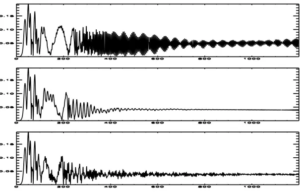
be summarized in this way: until t < τp the electric field energy damps exponentially
according with the linear Landau theory; when t ' τp non linear effects come into
play and the electric field energy, while is damped, begins to oscillate with a period of the order of τp; when t → ∞, as γ(t) → 0, the amplitude of the oscillations decreases
1.2.3
Long time evolution of Landau damping
In the previous sections we’ve seen that the relations between the characteristic times scales of the system, Landau damping time τL, trapping time τp and the wave
oscil-lation period τ0 = 1/ω, determine the way in which the system develops. Until now
we have described two cases: 1) when τp >> τL >> τ0, where the linear Landau’s
theory remains valid because the electrostatic wave is completely damped before par-ticles can be trapped in the potential wells; 2) when τL >> τp >> τ0, for which
particles are rapidly trapped before the wave starts to be damped, for which, at t about τp, the Landau theory is no longer valid [4]. The result of this last case is that
the wave amplitude, at large times, reaches a constant nonzero value. This regime is called O’Neil regime. In this section we want to discuss the intermediate regime when τp ∼ τL >> τ0. The theory has been developed by Lancellotti and Dorning [5]
in 1998. They found that there is a threshold for the initial perturbation amplitude: when initial amplitude is down the threshold there will be Landau’s regime while if it is above the threshold we will have O’Neil regime. Also in this case, due to the math-ematical difficulties to solve the nonlinear Vlasov-Poisson system of equations, it has been necessary make use of some approximations to solve the problem analytically. The Lancellotti and Dorning theory is based on the assumption that the electric field can be decomposed in a transient part ¯T and in a time-asymptotic part ¯A such that E(x, t) = ¯A(x, t) + ¯T (x, t). The decomposition allows to obtain an approximate
solu-tion through the linearizasolu-tion of the Vlasov and Poisson equasolu-tions for the transient part of the electric field ¯T . The Vlasov equation written in terms of ¯A + ¯T is given
by: ∂f ∂t + v ∂f ∂x − e me ¯ A∂f ∂v = e me ¯ T∂f0 ∂v (1.2.28)
where f0 is the initial distribution function. The ’transient linearization’ allows the
equations to remain uniformly valid even when t → ∞ because ¯T decays fast enough
before the distribution function deviates too much from the equilibrium one, while, the non linear part remains stored in the A term. Instead, as already discussed, in the Landau linearization the approximation of ∂f /∂v with ∂f0(v)/∂v ceases to be
valid at t ' τp.
and Dorning to compute analytically the existence of a threshold ²c for the initial
perturbation amplitude a that leads to the linear Landau damping regime ( ¯A = 0) if a < ²c, or to the O’Neil regime ( ¯A 6= 0) if a > ²c. This result justifies why in large
scale numerical simulations in some cases the electric field is damped to zero while in some others nonzero travelling waves are present. Furthermore they found that, if the amplitude of the wave is just above the threshold (a > ²c), the electron distribution
function evolves in time to reach a superposition of Bernstein-Greene-Kruskel (BGK) [?, 7] states in a ’coarse graining sense’, i.e. averaging the particle distribution function over the invariant curves discovered by Buchanan and Dorning [27] (as explained in Appendix A). The BGK states are exact undamped periodic wave solutions of the Vlasov-Poisson system which are stationary in the frame of reference moving at their phase velocity. They are Vlasov equilibria and therefore they are computed trough Vlasov and Poisson system of equations by setting ∂f /∂t = 0 (see Appendix A). Brunetti et al. [28] numerically studied this problem and verified the Lancellotti and Dorning theory [?] in the case of small amplitudes initial perturbations. They showed with the help of numerical simulations that the Vlasov-Poisson system reaches asymptotically in time a BGK state also in the case of large perturbation amplitudes, where Lancellotti and Dorning theory cannot be used, and studied the non linear stability of the system (side band instability).
1.3
Plasma wave echoes
In the study of Landau damping phenomenon an interesting paradox comes out: where does the energy associated to the electric wave goes when the wave is damped? At first sight, we could think that the energy has been converted into particles tem-perature. However this explanation is in conflict with fact that since the plasma is collisionless, the system conserves the entropy. The solution of the paradox can be found by calculating what happens to the distribution function when the damping takes place. It can be seen, in fact, that the excitation of an electric wave with wave number k1 modulates the electron distribution function leaving, in addition to terms
proportional to the electric field that damps away in time, a perturbation of the form
f1(v)exp(−ik1x + ik1vt). This last term, called the ballistic term, conserves the
and more rapidly as time goes on: f1(v)exp(ik1vt) → 0 when t increases. The
in-formations contained in the initial perturbation remain therefore hidden on the small scales fluctuations of the distribution function.
The experimental proof of this result is given by the echo phenomenon [2]. This phenomenon is, as a matter of fact, capable to bring back to the macroscopic scales part of the initial perturbation Landau damped away in time. In fact, if a second plasma wave is excited in the plasma after the first wave is Landau damped, an elec-tric field reappears in the plasma many Landau damping periods after the application of the second pulse. The generation of this new wave, called the echo, is due to the nonlinear constructive interference between the ballistic terms of the two waves dis-tribution functions. But how is generated this interference? Let’s take a collisionless plasma and excite an electric field of spatial dependence e−ik1x. When time goes on,
the electric field is Landau damped away and, as seen previously, it modulates the distribution function leaving a perturbation term of the form
δf1(1)(x, v, t) = f1(v)exp(−ik1x + ik1vt) . (1.3.1)
If at time τ we excite a second electric field with spatial dependence eik2x, it will
damp away in time, leaving a new perturbation in the electron distribution function. This second wave will modulate the unperturbed part of the distribution, as made by the first wave, producing a first order term of the form f2(v)exp(ik2x − ik2vt).
Furthermore it will modulated also the first order perturbation δf1(x, v, t) producing
a second order distribution function perturbation of the form
δf(2)(x, v, t) = f
1(v)f2(v)exp(i(k2 − k1)x + ik2vτ − i(k2− k1)vt) . (1.3.2)
Both the first order perturbations give no contribution to the electric field, because the velocity integral over them for large t will phase mix to zero. Instead, the second order one, provides a contribution to the electric field, but only when time t reaches the value τ0 = τ k
2/(k2− k1). In fact, when t < τ0, also the second order perturbation
is a highly oscillatory function as the first order perturbations, and hence its velocity integral tend to zero when t increases. However, when t approaches the time τ0,
the second order perturbation stops to be a highly oscillatory function because the exponent i(k2 − k1)x + ik2vτ − i(k2 − k1)vt vanishes at t = τ0. So, at this time,
the velocity integral over this term will no more phase mix to zero, leading to the appearance again of an electric field, i.e. the echo. Then, after a certain time interval, the second order perturbation term comes back to be again an highly oscillatory function since its velocity integral will again phase mix to zero.
The first analytical study of the temporal echo phenomenon is due to Gould, O’Neil and Malmberg in 1967 [1, 2]. Using the Vlasov and Poisson equations, they derived the electric potential of a second order echo. Making a brief review of this theory we will show how to get the echo potential. The theory assumes the plasma to be collisionless, one dimensional and that ions are at rest forming a neutralizing background. The electron distribution function is expanded in terms of an equilibrium homogeneous distribution, fe(x, v, t = 0) = f0(v) plus a perturbation term f1(x, v, t).
The total potential φ includes the potential due to the plasma charge distribution
ρ = eR f dv and an externally produced potential φext containing the two external
pulse we want to perturb the system with. The external potential, composed by one pulse of wave number k1 excited at t = 0 and a second one with wave number k2
applied after τ times from the first, takes the form:
φext= φk1cos(k1x)δ(ωpet) + φk2cos(k2x)δ[ωpe(t − τ )] (1.3.3)
where δ is the Dirac function.
The 1D-1V Vlasov - Poisson system, with fixed neutralizing protons, becomes:
∂f ∂t + v ∂f ∂x + e me ∂φ ∂x ∂f ∂v = 0 (1.3.4) ∂2φ ∂x2 = ∂2φ ext ∂x2 + 4πe µZ f dv − n0 ¶ . (1.3.5)
By taking the Fourier and Laplace transforms of Vlasov and Poisson equations, sub-stituting ˜fk(v, p) calculated from Vlasov equation in Poisson one and expanding the
compute the second order potential (for the detailed computation see Appendix B) for the wave number k3 = k2 − k1 (the one associated to the echo), obtaining:
φk3(2)(t) = φk1 ωpeeλD T τ φk2k41k2 T k3(k1+ k3)2 × ×−(k3/k1)γ(k1)e γ(k1)k3/k1(τ0−t)cos[ω(k 1)(k3/k1)(τ0− t) + δ {[ω2 pe(k3− k1)/(k3+ k1)]2+ γ(k1)2}{1/2} f or t < τ0 × γ(k3)eγ(k3)(t−τ 0) cos[ω(k3)(t − τ0) + δ0 {[ω2 pe(k3− k1)/(k3+ k1)]2+ γ(k3)2}{1/2} f or t > τ0 (1.3.6) where tan(δ) = γ(k1)(k3− k1)/[ωpe(k3+ k1)] tan(δ0) = γ(k 3)(k1− k3)/[ωpe(k3+ k1)]. (1.3.7)
We observe that the echo is symmetric in time only when k1 is exactly equal to
k3, otherwise it grows up at the rate exp[γ(k1)k3/k1(τ0− t)] and damps at the rate
exp[γ(k3)(t − τ0)].
This theory is based on the collisionless Vlasov equation, and looses its validity when collisional effects are enough ”rapid” to destroy the phase informations stored in the ballistic terms before the echo can appear. In order to investigate the importance of collisions in the long time dynamics of a weakly collisional plasma, it is possible to add a collisional operator to the Vlasov equation. O’Neil developed an analytical weakly collisional theory [?] for two small angle collisional processes: Coulomb col-lisions and microturbulence. These collisional processes result particularly effective at smoothing the distribution function ballistic term (large velocity gradients of the distribution function) and therefore, at destroying the plasma wave echo. With this theory, O’Neil computed how the presence of Coulomb collisions and microturbulence
affect the echo, as we will show in the rest of this section. Even in this case, the the-ory is developed in the limit of a one dimensional unmagnetized plasma. The part of the theory that we discuss here refers to the case of second order temporal echoes in presence of Coulomb collisions. A Fokker-Plank operator [29, 30, 31] of the form
FP(f ) = − ∂
∂v[D1f ] + ∂2
∂v2[D2f ] (1.3.8)
has been chosen by O’Neil to represent small-angle collisions. When this operator is applied to a free streaming perturbation as f1(x, v, t) = exp(ikx − ikvt), the leading
term of the operator at large times is the second velocity derivative. Therefore, at large times the Fokker-Plank operator acting on f1(x, v, t) can be approximate as:
FP(exp(ixk − ikvt)) ' −D2k2t2exp(ikx − ikvt) (1.3.9)
where the coefficient of exp(ikx − ikvt) can be interpreted as the effective collision frequency νef f(k, t) = D2k2t2.
Before presenting the analytical steps for obtaining the echo potential expression, some assumptions have to be made. These assumption are useful to make easier the calculation. The first, coming from the choice of considering a weakly collisional plasma, is that, during the Landau damping phase, collisional damping must be negligible, i.e. γL−1νef f << 1. This assumption means that the theory is valid only for
regimes in which the coefficient D2is sufficiently small so that, while Landau damping
is acting, collisions practically produce no effect. Second, the time τ0 between the
application of the first pulse and the appearance of the echo must be much longer than the Landau damping time, i.e. τ0γ
L >> 1. This last assumption is necessary to
ensure that collisions have a relevant effect on the echo. In fact, since D2 is small the
effect of collisions can be felt only when the time t is large enough to overcome the smallness of D2. Hence, if τ0 is too small (i.e. νef f is small), collisions have no time
to affect the ballistic terms before the echo is formed.
With these assumption, O’Neil first used collisionless theory to obtain the initial form of the electron distribution function perturbation resulting from the application of the two pulses and then used the Fokker-Plank equation without electric field
driving terms to determine the collisional damping affecting the perturbations during the free streaming.
If we excite in the plasma a first pulse of the form φk1cos(k1x)δ(ωpet), collisionless
theory predicts that the form of the first order electron distribution function streaming perturbation will be:
fk(1)(v, t) = e me φk1[δ(k − k1) + δ(k + k1)]ik 2ωpe²(k, −ikv) ∂f0 ∂v e −ikvt (1.3.10)
where, as above, f0(v) is the initial Maxwellian distribution function and ²(k, −ikvt)
is the dielectric function. Using equation C.0.21 as the initial condition, the electron distribution function streaming perturbation evolves according to the homogeneous Fokker-Plank equation
∂fk
∂t + ivkfk− FP(fk) = 0 (1.3.11)
until the excitation of the second pulse. Substituting equation C.0.21 in C.0.22 one obtains: fk(1)(v, t) = e me φk1[δ(k − k1) + δ(k + k1)]ik 2ωpe²(k, −ikv) ∂f0 ∂v exp µ −ikvt − Z t 0 νef f(k, t0)dt0 ¶ (1.3.12) where νef f(k, t) = D2k2t2. The collisional damping factor that appears in the previous
equation was already determined by Karpman [32] and Su and Oberman [33] for a streaming perturbation damped by Coulomb collisions and by Dupree [31] for the microturbulence case.
When also the second pulse, of the form φk2cos(k2x)δ[ωpe(t − τ )] is excited in
the plasma, it will generate a first order streaming perturbation of the same type of equation C.0.21 but with k2 instead of k1 and t − τ instead of t, and a second order
one derived from the modulation of the perturbation already left by the first pulse. This second order term is produced only for wave numbers k1+ k2 and k2− k1 but,
as already mentioned before, the one for which the echo is generated will be only
fk(2)3 (v, t) = µ e me ¶2 k1k2φk1φk2ik1τ ∂f0 ∂v exp¡−ik3v(t − τ ) + ik1vτ − Rτ 0 νef f(k1, t0)dt0 ¢ 4ω2 pe²(k2, −ik2v)²(−k1, ik1v) . (1.3.13) Substituting equation C.0.24 as initial condition in the homogeneous Fokker-Plank, equation C.0.22, one obtains:
fk(2)3 (v, t) = µ e me ¶2 k1k2φk1φk2ik1τ ∂f0 ∂vexp(−ik3v(t − τ ) + ik1vτ )× × exp ³ −R0τνef f(k1, t0)dt0− Rt τ νef f(k1, k2, τ, t0)dt0 ´ 4ω2 pe²(k2, −ik2v)²(−k1, ik1v) (1.3.14)
where νef f(k1, k2, τ, t0) = D2[−k3(t0 − τ ) + k1τ ]2 is the effective collision frequency
that one obtains when the Fokker-Plank operator acts on the second order ballistic term exp[−ik3v(t − τ ) + ik1vτ ]. To determine the echo potential we divide equation
C.0.25 by ²(k3, −ik3v) (to account for the self-consistent field associated to the echo
itself), and inserting it in Poisson equation. The potential calculated at time τ0 at
which the echo occurs, results:
φk3 = ek2 1k2φk1φk2iτ 4mk2 3 Z +∞ −∞ dv∂f0 ∂vexp[ik3v(τ 0− t)]× × exp ³ −R0τνef f(k1, t)dt − Rτ0 τ νef f(k1, k2, τ, t)dt ´ ²(k2, −ik2v)²(−k1, ik1v)²(k3, −ik3v) . (1.3.15)
If the diffusion coefficient D2 is independent of time, as occurs for Coulomb
col-lisions, the exponential term containing the collisional damping rate can be easily evaluate obtaining: exp à − Z τ 0 νef f(k1, t)dt − Z τ0 τ νef f(k1, k2, τ, t)dt ! = exp µ −D2(v) k2 1k2τ3 3k3 ¶ . (1.3.16)
In the case where D2 is also independent of velocity, the collisional damping factor
can be extracted integral sign. In this way, the shape of the echo results the same as the one obtained in the collisionless case but the amplitude is reduced by a factor
exp µ −D2 k2 1k2τ3 3k3 ¶ . (1.3.17)
When instead D2 is a function of velocity, the amplitude as well as the shape of
the echo will result different from the collisionless ones. O’Neil found that in this case the collisional damping reduces the wings of the echo more that the peak of the echo. The existence of plasma echoes was proved experimentally by Gould, O’Neil and Malmberg in 1967 [2]. In this work they also verified some of the echo properties predicted by the theory, even for echoes of higher orders. Many other studies are made on the echo phenomenon, as theoretical as experimental (see for example [34, 35, 36, 38, 39, 40]).
1.4
Two stream instability
The two stream instability is a velocity-space instability driven by electron momentum anisotropy. To generate a two stream instability in a collisionless plasma we take, as the initial anisotropic equilibrium, two electron streams of density na and nb drifting
with uniform velocities Vaand Vbin opposite direction on a background of neutralizing
protons, such that the initial total current in the plasma is zero. Because of the initial anisotropy of the electron distribution function, if we perturb longitudinally the system with a small amplitude electrostatic wave, the amplitude of the perturbation begins to increase, corresponding to the development of the two stream instability. We will see, however, that only a limited range of wavelengths are unstable. This increase in the electric field energy is obtained to the disadvantage of electrons kinetic energy. During the development of the instability, in fact, the electrons of the two streams begin to be accelerated and decelerated by the wave field. When the amplitude of the electric field becomes large enough to trap less energetic electrons (i.e. when eΦ is about mv2
e/2, where veis the velocity of an electron), the instability starts to saturate
electron trapping, driven by kinetic effects, necessitate of a kinetic approach, while the initial development of the instability (linear regime) can be described also by a fluid theory if we’re dealing with a cold plasma. In the following of this section we compute the dispersion relation by using the linearized kinetic equations. If the direction of propagation of the electrostatic perturbation is chosen to lie along the same direction of the two electron streams, the system can be easily described in a one dimensional space using the Vlasov and Poisson equations. Considering the neutralizing ions to be of infinite mass, we can neglect their motion. In this way, the analysis is restricted only to high frequency effects. We take the Vlasov Poisson system of equations 1.1.1, 1.1.2 where n0, feand φ represent the protons density, the electron distribution
function and the electrostatic potential, respectively. The linearized equations can be obtained expressing the distribution function fe and the electric potential φ as
fe(x, v, t) = fe0(x, v, t) + ²fe1(x, v, t) and φ(x, t) = φ0(x, t) + ²φ1(x, t) and taking the
Fourier transform with respect to the spatial variables and the Laplace transform in time. The resulting equations are:
(p + ikv) efek= fek(k, v, t = 0) + ik e me ∂fe0 ∂v fφk = 0 (1.4.1) k2fφ k = 4πe Z f fekdv (1.4.2) where fek(v, t) = 1 2π Z fe1(x, v, t)exp(−ikx)dx (1.4.3) e fek(v, p) = 1 2π Z ∞ 0 fek(v, t)exp(−pt)dt <(p) > p0 (1.4.4) φk(t) = 1 2π Z φ1(x, t)exp(−ikx)dx (1.4.5) e φk(p) = 1 2π Z ∞ 0 φk(t)exp(−pt)dt <(p) > p0 (1.4.6)
Choosing the initial electron distribution function as
and assuming, for simplicity, that the two electron streams have equal density (na0 =
nb0 = 1/2) and equal but opposite velocities (Va0 = −Vb0 = V0/2), the dispersion
relation resulting from equations 1.4.1, 1.4.2 is:
1 = ω 2 pe 2(ω − kV0/2)2 + ω 2 pe 2(ω + kV0/2)2 +ω 2 pi ω2 (1.4.8)
where the last term can be neglected since ω2 >> ω2
pi. The roots of equation 1.4.8
are: ω2 = ωpe2 2 + k2V2 0 4 ± r (ω 2 pe 2 + k2V2 0 4 )2+ k2V2 0 4 (ω2pe− k2V2 0 4 ) (1.4.9)
To generate the instability it is necessary that equation 1.4.9 admits almost one positive complex root. This can be obtained if:
|kV0| < 2ωpe (1.4.10)
This condition says that unstable modes will correspond to wavelengths in the range 0 < λ < πV0/ωpe with k = 2π/λ. When V0 → 0 the grow rate vanishes, as expected
and we retrieve plasma oscillations at ω = ωpe since we neglected thermal effects. The
maximum grow rate is achieved for kV0 = 3ωpe/
√ 2 and is equal to ωi,max = ωpe √ 8 . (1.4.11)
As in Landau damping phenomenon, when the wave is large enough to trap the particles, the linear theory breaks down. In fact, the linear Vlasov theory (see section 1.1) is based on the assumption that the orbits of plasma particles are only slightly perturbed by the wave field. On the other hand, when trapping comes into play, the trajectories are strongly deformed: the free streaming motion is converted in quasi-periodic orbits. This process corresponds, in phase space, to the development in the distribution function of coherent structures called vortices corresponding, in
the particle density, to phase space holes [41]. Such coherent structures are associated to BGK states for which the density of trapped particles is lower than the density of free and reflected particles [42]. We can distinguish two kinds of vortices: those generated in the electron distribution function called electron holes, and those of ion distribution function called ion holes. Electron holes are associated to a positive potential perturbation while ion holes to a negative potential one. In our case, where ion are fixed, obviously only electron vortices can be developed. We note that the generation of an hole is formally forbidden by the Vlasov theory and, therefore, it needs of dissipative effects.
The two stream instability can generate more than one vortex. The number of these coherent structures depends on the spatial dimension of the plasma model. All vortices are generated with the same velocity and develop close enough to each other to interact. Berk et al. have shown, in 1970, that phase space holes attract each other [43]. The basic idea of this demonstration is the following. Looking at the particle density, one can represent the holes of the phase space as assemblies of particles with charge −q and mass −m on a stable band of particles of mass m and charge q. The particles that represent the holes will interact electrostatically. The electrostatic interaction between particles of the same charge and negative mass is attractive. Hence each phase space hole, since it is considered as to be ”composed” by such particles, will tend to remain a coherent structure. Furthermore, since every phase space holes in the particle density will be made of the same kind of particles with negative charge and negative mass, they will attract each other. This attraction process will lead to collisions among holes which, if in the system some dissipation comes into play, generate a merging process. Bertrand et al. [13] demonstrated through numerical and analytical studies of the two stream instability in the case of a collisionless 1D umagnetized plasma, where ions are considered as a neutralizing fixed backgrund, that BGK states composed by a number of vortex N ≥ 2 are always unstable. They observed from numerical simulations, that this fact induced a coalescence process leading to the formation of a final stable single vortex.
1.4.1
Ion-acoustic waves
Let’s consider the same one dimensional unmagnetized collisionless plasma system described previously but, this time, assuming also the ions free to move. In this