Titolo
Sviluppo di un modello di dinamica di nocciolo per un DEMO LFR
Ente emittente
CIRTEN
PAGINA DI GUARDIA
Descrittori
Tipologia del documento:
Rapporto Tecnico
Collocazione contrattuale:
Accordo di programma ENEA-MSE: tema di ricerca "Nuovo
nucleare da fissione"
Argomenti trattati:
Reattori nucleari veloci
Generation IV reactors
Reattori e sistemi innovativi
Sommario
E' stato sviluppato, per il reattore dimostrativo raffreddato a piombo, un modello semplificato di
dinamica di nocciolo che permette un approccio preliminare alle problematiche di controllo del
sistema. Questo consente un'analisi relativamente veloce della dinamica e della stabilità del
sistema, che non può essere tralasciata in fase di progettazione. Il modello adottato, basato
sull'approssimazione point-kinetics e su un modello di scambio di calore a temperature medie, è
comunque in grado di considerare i principali feedback che controreazionano la variazione di
reattività a fronte dei principali transitori operativi ed incidentali, tenendo conto sia della
neutronica, della termo-idraulica e della espansione termo-meccanica.
Sono state quindi analizzate le risposte del reattore (in termini di escursione di temperatura del
combustibile MOX e della guaina in acciaio ferritico-martensitico T91) ad eventi iniziatori di
transitori, sia ad inizio sia a fine ciclo, implementando
il
modello sviluppato sulla piattaforma
MATLAB/SIMULINK®.
Note
REPORT LP3.G2 - PAR 2007
Autori:
Sara Bortot*, Antonio Cammi*, Patrizio Console Camprini**, Carlo Artioli***
*Politecnico di Milano, Dipartimento di Energia, Sezione Ingegneria Nucleare-CeSNEF
"Università di Bologna, Dipartimento di Ingegneria Energetica, Nucleare e del Controllo Ambientale (DIENCA)
***ENEA Copia n.
o
REV. EMISSIONE DESCRIZIONE In carico a: NOME FIRMA NOME FIRMA NOMENA
~. ~ontiNA
~?l.
9.
W\O)--F-IRM-A--+----~
YJ
H-::
-+-r-
dl
f
l
+
7l
rl
'
-
J
-t---1
VIWo .•DATA CONVALIDA APPROVAZIONE
2
1
PER LA
R
ICERCAT
ECNOLOGICAN
UCLEAREPOLITECNICO
DI
MILANO
DIPARTIMENTO DI ENERGIA, Sezione INGEGNERIA NUCLEARE-CeSNEF*
UNIVERSITA’ DI BOLOGNA
DIPARTIMENTO DI INGEGNERIA ENERGETICA, NUCLEARE e del CONTROLLO AMBIENTALE (DIENCA)**
ENEA
Centro Ricerche Bologna***
Sviluppo di un modello di dinamica di nocciolo per un
DEMO LFR
Sara Bortot*, Antonio Cammi*, Patrizio Console Camprini**, Carlo Artioli***
CIRTEN-POLIMI RL 1138/2010
Milano, Agosto 2010
Lavoro svolto in esecuzione della linea progettuale LP3 punto G2 – AdP ENEA MSE del 21/06/07 Tema 5.2.5.8 – “Nuovo Nucleare da Fissione”
LP3.G2 - 2 - CERSE-POLIMI RL-1138/2010 INDEX EXECUTIVE SUMMARY...‐ 3 ‐ 1 INTRODUCTION ...‐ 4 ‐ 2 DEMO DYNAMICS STUDY ...‐ 4 ‐ 2.1 DEMO core configuration ...‐ 7 ‐ 2.2 Reactivity coefficients...‐ 7 ‐ 2.3 Mathematical model ...‐ 7 ‐ 2.4 Simulations and results...‐ 7 ‐ 2.5 DEMO core open loop stability... ‐ 7 ‐ 3 NEUTRON KINETICS EVALUATIONS ...‐ 4 ‐ 3.1 Computational Schemes...‐ 7 ‐ 3.2 Results ...‐ 7 ‐ 4 PRELIMINARY EVALUATION OF CORE MECHANICS‐RELATED ASPECTS ...‐ 4 ‐ 4.1 Mathematical model ...‐ 7 ‐ 4.2 Simulations and results...‐ 7 ‐ 4.3 DEMO core open loop stability... ‐ 7 ‐ 5 CONCLUSIONS ...‐ 4 ‐ REFERENCES...‐ 4 ‐ NOMENCLATURE ...‐ 4 ‐ BIBLIOGRAPHY ...‐ 4 ‐ ANNEX A ...‐ 4 ‐
LP3.G2 - 3 - CERSE-POLIMI RL-1138/2010
E
XECUTIVES
UMMARYThis document presents the status of development of a core dynamics model for a Generation IV Lead-cooled Fast Reactor (LFR) demonstrator (DEMO). A preliminary approach to the simulation of a core dynamics has been developed to provide a helpful tool in this early phase of the reactor pre-design -in which all the system specifications are still considered to be open design parameters-, allowing a relatively quick, qualitative analysis of dynamics and stability aspects that cannot be left aside when refining or even finalizing the system configuration.
Reactivity coefficients and kinetics parameters have been estimated for both Beginning of Cycle (BoC) and End of Cycle (EoC) core configurations (see also G. Grasso et al., “Progettazione concettuale di un nocciolo di impianto dimostrativo di LFR”, linea progettuale LP3 – punto G1). A simplified lumped-parameter model reckoning with all the main feedbacks following a reactivity change in the core has been then developed to treat both neutronics and thermal-hydraulics: indeed, the point-kinetics approximation has been employed and an average-temperature heat-exchange model has been implemented. The latter sub-systems have been coupled and DEMO core responses to operational transient initiators -such as coolant inlet temperature perturbation or control rod withdrawal- at BoC and EoC have been finally analyzed using the MATLAB/SIMULINK® tool.
Space-time and point kinetics models have been then employed to provide preliminary indications of the core local behaviour following a transient, so as to primarily assess the excursions that MOX fuel and T91 ferritic-martensitic steel (FMS) cladding temperatures undergo, as they are subject to the most restricting technological constraints, whose respect must be guaranteed.
A further study has been begun aimed at addressing also the dynamic mechanical behaviour of DEMO core, by considering expansions and contractions instantaneous with temperature variations, i.e. neglecting mass inertia effects.
LP3.G2 - 4 - CERSE-POLIMI RL-1138/2010
1
INTRODUCTIONThe Lead-cooled Fast Reactor (LFR), being one of the six innovative systems selected by the Generation IV International Forum (GIF), is under development worldwide as a very promising fast neutron system to be operated in a
closed fuel cycle [1]. In particular, within the 6th and 7th EURATOM Framework Programmes the European LFR
community is proposing the ELSY - European Lead-cooled SYstem concept [2], an innovative 600 MWe pool-type
LFR fully complying with Generation IV goal of sustainability and, in particular, aiming at no net production of Minor Actinides (MAs).
As recognized by the Strategic Research Agenda worked out by the European Sustainable Nuclear Energy Technology Platform (SNETP), LFR complete development requires -as a fundamental intermediate step- the realization of a demonstration plant (DEMO), intended to validate LFR technology as well as the overall system behaviour [3]. Indeed, a demonstration reactor is expected to prove the viability of technology to be implemented in the First-of-a-Kind industrial power plant.
In order to define a first reference configuration of a GENIV LFR DEMO, an I-NERI (International Nuclear Energy Research Initiative) agreement between the National Agency for the New Technologies, Energy and Environment (ENEA) and Argonne National Laboratory (ANL) has been signed in 2007. From the Italian side the work is being carried out in the frame of the national R&D program on “New Nuclear Fission” supported by the Italian Minister of Economic Development (MED) through a general Agreement with ENEA and the Italian University Consortium (CIRTEN).
In such a context, a reference configuration for a 300 MWth pool-type LFR DEMO is being developed and a static
neutronics and thermal-hydraulics characterization has been accomplished [4].
Due to the need of investigating reactor responses to temperature transients, a preliminary approach concerning the simulation of DEMO core dynamics has been developed, in order to provide a helpful tool in this early phase of the reactor pre-design -in which all the system specifications are still considered to be open design parameters-, allowing a relatively quick, qualitative analysis of fundamental dynamics and stability aspects that cannot be left aside when refining or even finalizing the system configuration.
In this perspective, reactor dynamics is of primary importance for the study of plant global performances and for the design of an appropriate control system, since it explains the interactions among input and output variables and the nature of the basic dynamic relationships.
Many effects must be taken into account simultaneously for an accurate simulation: the coupling of different physical subsystems (i.e., neutronics, thermal-hydraulics, etc.) is concerned with the complexity of the large number of phenomena involved, and with the approximations necessarily employed to implement the model (geometrical arrangement description as well as mathematical and numerical treatment).
A simplified lumped-parameter model reckoning with all the main feedbacks following a reactivity change in the core has been then developed to treat both neutronics and thermal-hydraulics. Indeed, it has been assumed that neutron time fluctuations and spectrum are independent of spatial variations and neutron level, respectively. Accordingly, the core has been considered as a lumped source of neutrons with prompt heat power, with neutron population and neutron flux related by constants of proportionality, leading to the point-kinetics approximation to be employed [5].
A zero-dimensional approach has been adopted to treat also the system thermal-hydraulics. Some simplifying hypotheses have been assumed and a single-node heat-exchange model has been implemented by accounting of three
LP3.G2 - 5 - CERSE-POLIMI RL-1138/2010 distinct temperature regions –corresponding to fuel, cladding and coolant-, enabling reactivity feedback to include all the major contributions. In line with the point model concept, fuel, cladding and coolant temperatures have been assumed to be functions separable in space and time.
Neutron kinetics has been then coupled with heat transfer dynamics through reactivity feedback coefficients -generated by change in neutron cross sections due to fuel Doppler and coolant density effects and by core thermal expansions-, which have been estimated for both Beginning of Cycle (BoC) and End of Cycle (EoC) core configurations by means of ERANOS (European Reactor ANalysis Optimised System) deterministic code ver. 2.1 [6] coupled with JEFF-3.1 data library [7], as well as the corresponding kinetics parameters.
DEMO dynamic behaviour has been studied through a simplified linearized model -based on a small perturbation approach-, which has been handled in terms of state, input and output variables, according to the theory of linear systems. The Laplace-transformed equations have been solved simultaneously by means of a matrix equation so as to evaluate the system representative transfer functions. Core responses to operational transients initiators -such as coolant inlet temperature stepwise perturbation or control rod withdrawal- at BoC and EoC have been finally analyzed using the
MATLAB/SIMULINK® tool [8, 9], in order to assess the excursions that MOX fuel and T91 ferritic-martensitic steel
(FMS) cladding temperatures undergo, since they are subject to the most restricting technological constraints whose respect must be guaranteed during any operational transient [4]. The analysis of DEMO core sub-system open-loop stability has ultimately been performed.
A preliminary study of DEMO core kinetics has been then associated to dynamic investigations: the ERANOS KIN3D module [10] has been employed to accomplish simulations of reactor transients induced by both fuel temperature and coolant temperature variations, and a control rod complete withdrawal and insertion.
Material density and temperature distributions obtained from the previous coupled point-kinetics and thermal-hydraulics model have been employed to compute effective neutron cross-sections for reactor sub-regions that have been used as input data for core neutronics calculations.
Finally, an alternative dynamic model of DEMO has been implemented in order to approach the problem of the core mechanical behaviour, which has been initially coped with by neglecting mass inertia effects.
2
DEMO DYNAMICS STUDY2.1 DEMO core configuration
In the current design, DEMO features a 300 MWth MOX-fuelled core, composed by wrapper-less square fuel
assemblies (FAs) with pins arranged in a square lattice; 10 FAs with 29.3 vol.% Pu fraction constitute the inner zone, and 14 FAs with 32.2 vol.% Pu fraction compose the outer zone.
As far as FA design, fuel pins are arranged in a 28×28 square lattice, every FA being provided with 4 structural uprights at corners connected with the central FMS T91 box beam replacing 6×6 central positions.
Two different and independent control rod systems guarantee the required reliability for reactor shut-down and safety: 4
passive B4C (90 at.% enrichment in 10B) Finger Absorber Rods (FARs) carry out exclusively SCRAM purposes, being
positioned outside the active core in normal operation; 20 motorized B4C (42 at.% enrichment in 10B) FARs are
demanded for cycle reactivity swing control and safe shut-down, 16 of which being inserted for half active height (BoC reference configuration) or positioned 1 cm above the active core (EoC reference configuration) respectively.
LP3.G2 - 6 - CERSE-POLIMI RL-1138/2010 Fig. 1 shows (on the left) a radial section of the core composed by 24 FAs surrounded by dummy assemblies, and (on the right) a bi-dimensional RZ representation of the vertical section that yields a useful scheme for the main structural zones.
Fig. 1. Core layout (left) and 2D RZ cylindrical section (right); dimensions in cm.
In Table I the main DEMO core specifications are summarized.
TABLE I
DEMO major core specifications, cold dimensions (20 °C).
Parameter Value Unit
Thermal Power 300 MWth
Average Coolant Outlet Temperature 480 °C
Coolant Inlet Temperature 400 °C
Average Coolant Velocity 3.0 m s-1
Cladding Maximum Temperature 600 °C
Cladding Outer Diameter 6.00 mm
Cladding Thickness 0.34 mm
Pellet Outer Diameter 5.14 mm
Pellet Hole Diameter 1.71 mm
Fuel Column Height 650 mm
Fuel Rod Pitch 8.53 mm
Number of Pins/FA 744 -
FMS box beam inner width 45.65 mm
FMS box beam outer width 48.65 mm
Number of Inner/Outer FAs 10/14 -
LP3.G2 - 7 - CERSE-POLIMI RL-1138/2010
2.2 Reactivity coefficients
Neutronics analyses have been performed by means of ERANOS deterministic code ver. 2.1 in conjunction with JEFF-3.1 data library.
Multi-group cross-sections associated to every reactor zone shown in Fig. 1 have been retrieved from ECCO (European Cell COde) [11] calculations. A very refined cell description has been adopted for both FAs and subcritical zones surrounding the active core (with the exception of dummy radial reflector assemblies): they have been described by an accurate heterogeneous geometry model, whereas the remaining ones (namely ‘Foot FA’, ‘Dummy Belt’, ‘Barrel’ and ‘External Lead’) have been described by a homogeneous cell geometry model. In both cases, ECCO computations have been carried out by treating the main nuclides with a fine energy structure (1968 groups) and condensing the obtained cross-sections into 33 groups.
The reference working temperatures which have been assumed are the following: in the active core zone, 900 °C for the fuel, 440 °C for structures and coolant, 480 °C for the cladding; for subcritical cells, 400 °C for zones below the active zone, 480 °C above the active zone, and 440 °C for lateral zones.
ECCO evaluations have finally been used to set tri-dimensional core models up; then the whole system has been solved through nodal transport calculations by means of the ERANOS TGV/VARIANT module [12].
In the reference configurations the reactor is characterized by a multiplication factor keff = 1.00033 (ρ = 33 pcm) and
keff = 1.00093 (ρ = 93 pcm) at BoC and EoC, respectively.
In order to estimate the Doppler and the coolant density feedback effects, the following deviations from the nominal parameters have been applied:
- fuel temperature raise (variation: + 326.85 K);
- coolant density reduction in the active core zone (variation: - 5%).
Furthermore, elementary perturbations have been introduced in order to figure radial and axial expansion reactivity coefficients through a “partial derivative” approach. Such a method is based on the main hypothesis of superposition principle validity and of linear response of the system within the interval defined by the reference and the perturbed configurations as well.
The following elementary perturbations have been applied:
- core radial extension by scaling all radial dimensions, with nominal densities (variation: + 2.5%); - core axial extension by scaling all axial dimensions, with nominal densities (variation: + 5%); - fuel density reduction (variation: - 5%);
- steel density reduction (variation: - 5%); - absorber density reduction (variation: - 10%).
The latter have been then composed to compute the main reactivity coefficients as described in the following sections.
Doppler Coefficient
The Doppler effect can be evaluated according to the relation:
T dT
LP3.G2 - 8 - CERSE-POLIMI RL-1138/2010 With respect to the considered temperature variation (from 1173.15 to 1500 K), the Doppler coefficient results
αD = - 0.177/- 0.202 pcm K-1 at BoC and EoC, respectively.
Since the reactivity change is strongly dependent (logarithmic behaviour) on the temperature variation involved, the Doppler constant α is provided owing to its more general applicability: α = - 235/- 268 pcm. Its rather low value is
justified by the high Pu fraction, which weakens the effect of 238U macroscopic absorptions in epithermal region.
Coolant Density Coefficient
The coolant density reactivity coefficient can be computed by referring to the following expression:
dT d dT d cool cool cool cool coolant ⎟⎟ ⎠ ⎞ ⎜⎜ ⎝ ⎛ Ρ Ρ ⎟⎟ ⎠ ⎞ ⎜⎜ ⎝ ⎛ Ρ Ρ ∂ Ρ ∂ = δ δ ρ (2)
Considering the elementary perturbations and the coolant thermal expansion [13], the coolant density coefficient results
αL = - 0.120/- 0.141 pcm K-1 at BoC and EoC, respectively.
Radial Expansion Coefficient
Despite the fact that no diagrid is foreseen in DEMO design, the traditional reactivity effect due to its radial expansion can be calculated thanks to the continuous lattice formed by FA foots [14] according to:
⎪ ⎪ ⎭ ⎪ ⎪ ⎬ ⎫ ⎥ ⎥ ⎥ ⎥ ⎥ ⎦ ⎤ ⎟⎟ ⎠ ⎞ ⎜⎜ ⎝ ⎛ Ρ Ρ ∂ ∂ ⎟⎟ ⎠ ⎞ ⎜⎜ ⎝ ⎛ − + ⎟⎟ ⎠ ⎞ ⎜⎜ ⎝ ⎛ Ρ Ρ ∂ ∂ + ⎟⎟ ⎠ ⎞ ⎜⎜ ⎝ ⎛ Ρ Ρ ∂ ∂ ⎪ ⎪ ⎩ ⎪ ⎪ ⎨ ⎧ ⎢ ⎢ ⎢ ⎢ ⎢ ⎣ ⎡ + ⎟ ⎟ ⎠ ⎞ ⎜ ⎜ ⎝ ⎛ Ρ Ρ ∂ ∂ − ⎟ ⎠ ⎞ ⎜ ⎝ ⎛ ∂ ∂ ≈ coolant coolant coolant steel steel absorber absorber fuel fuel in T diagrid f R R T l dT d δ ρ δ ρ δ ρ δ ρ δ ρ ρ ( ) 2 1 1 91 (3)
where the T91 linear expansion coefficient has been evaluated at the nominal lead inlet temperature [15].
The reactivity coefficient due to the diagrid-equivalent radial expansion results αR = - 0.871/- 0.923 pcm K-1 at BoC and
EoC, respectively.
An alternative value for the core radial expansion coefficient has been calculated considering the radial expansion to be
driven by the coolant inlet temperature Tl, leading to αR = - 0.886/- 0.939 pcm K-1 at BoC and EoC, respectively.
Axial Expansion Coefficient
The elementary reactivity variations have been properly combined in order to obtain the equivalent coefficient due to the core axial expansion according to:
LP3.G2 - 9 - CERSE-POLIMI RL-1138/2010 dT dL L Z Z dT T l T T dT d insertion insertion steell steel fuel fuel T T mat in mat out mat axial out mat in mat ∂ ∂ + ⎥ ⎥ ⎥ ⎥ ⎥ ⎦ ⎤ ⎟ ⎟ ⎟ ⎟ ⎟ ⎠ ⎞ ⎜ ⎜ ⎜ ⎜ ⎜ ⎝ ⎛ ⎟⎟ ⎠ ⎞ ⎜⎜ ⎝ ⎛ Ρ Ρ ∂ ∂ + ⎟ ⎟ ⎠ ⎞ ⎜ ⎜ ⎝ ⎛ Ρ Ρ ∂ ∂ ⎢ ⎢ ⎢ ⎢ ⎣ ⎡ − ⎟ ⎠ ⎞ ⎜ ⎝ ⎛ ∂ ∂ − ≈
∫
ρ δ ρ δ ρ δ ρ ρ *, *, ) ( 1 *, *, (4)The contribution of the dislocation of FARs due to their differential expansion with respect to the active core has been accounted of by considering the dilations of both the hot leg and the active core instantaneous [14], as follows:
core leg
hot
insertion dL dL
dL = − + (5)
where the first term has been calculated as:
dT T l T L
dLhot−leg = hot−leg( out)T91( out) (6)
and the dilation of the core portion interested by the insertion of FARs (assumed LFARs) has been written as:
dT dL L l dL fuel FARs Z L T core ⎟⎟ ⎠ ⎞ ⎜ ⎜ ⎝ ⎛ =
∫
91( ) (7)in the linked case, and
dT dL L l dT dL L l dL FARs fuel L MOX Z T core ⎟⎟ ⎠ ⎞ ⎜ ⎜ ⎝ ⎛ − ⎟ ⎟ ⎠ ⎞ ⎜ ⎜ ⎝ ⎛ =
∫
( )∫
( ) 0 0 91 (8)in the not-linked case, where the concerned linear expansion coefficients have been properly evaluated on the basis of both the steel- and fuel-related values in correspondence to the respective theoretical mean temperatures at steady-state [15, 16].
Coherently, the axial expansion coefficient turns out to be αZ = 0.009/- 0.195 pcm K-1 (BoC/EoC) in the linked case,
and αZ = 0.033/- 0.191 pcm K-1 (BoC/EoC) in the not-linked case.
2.3 Mathematical model
The model developed is based upon the fundamental conservation equations and employs a lumped parameters approach for the coupled kinetics (six delayed neutron precursor groups point reactor) and thermal-hydraulics, with continuous reactivity feedback due to temperature effects. A simplified block-scheme of DEMO primary system -assumed to consist only of the active core, disregarding both upper and lower plena- has been adopted: the thermal-hydraulics sub-system has been described by zero-dimensional, single phase, single channel conservation
LP3.G2 - 10 - CERSE-POLIMI RL-1138/2010 equations. Fuel, cladding and coolant temperatures have been determined through an energy balance over the average pin surrounded by coolant, in which reactor power is an input variable retrieved from reactor kinetics (coherently with the approximation of accounting only for the total power generated by fission, neglecting the contribution of decay heat). The so-calculated thermal-hydraulic parameters have been finally employed to insert the reactivity feedbacks into the neutronics equations, as shown in Figure 2.
H H Ψ Ψ CCii CORE T Tff TTcc TTll T Tinin δρ(t) δψ(t) δTin(t) δTf(t) δTc(t) δTl(t) δq(t) δTout(t) δTin(t) δH(t) δTf(t) δTc(t) δTl(t) δρ(t) δH(t) Kinetics Thermal-hydraulics Reactivity Input T Toutout
Fig. 2. DEMO core block scheme.
Neutron Kinetics Equations
The one prompt group point kinetics formulation of the neutron density can be written as [5]:
) ( ) ( ) ( 6 1 t C t n dt t dn i i
∑
+ Λ − = ρ β λ (9)the corresponding concentration of the six precursor groups of delayed neutrons being expressed as:
) ( ) ( ) ( t C t n dt t dC i i i i β −λ Λ = . (10)
As a further assumption, the system has been considered at steady-state for t ≤ 0.
A small perturbation approach has been applied, given that the point kinetics model is computationally efficient and can provide accurate results for small reactor perturbations when "true" time-dependent distributions of power and reactivity coefficients close to their steady-state distributions may be assumed.
Consequently, Eq. (9) and (10) have been perturbed around their steady-state solutions and then linearized obtaining seven linear equations describing the neutron kinetics behaviour in terms of dimensionless variables:
Λ + Λ + Λ − = ( ) 1
∑
( ) ( ) ) ( 6 1 t t t dt t d i i δρ δη β δψ β δψ (11)LP3.G2 - 11 - CERSE-POLIMI RL-1138/2010 ) ( ) ( ) ( t t dt t d i i i i λδψ λδη δη − = , (12)
being ψ = n(t)/n0 = q(t)/q0 and ηi = Ci(t)/Ci0.
Reactivity and Feedback Function
Consistently with the lumped parameter modelling employed, reactivity feedback has been expressed as a function of the mean values of fuel, cladding and coolant temperatures, and core inlet temperature. Moreover, externally introduced
reactivity has been simulated by the coefficient αH associated with the insertion length of an ideal control rod, which has
handled as a simple input parameter.
Under the hypotheses of small perturbations, reactivity depends linearly on constant coefficients associated with the respective parameter variation from its steady-state value; therefore, continuous reactor feedbacks have been calculated as follows (reference calculations):
H T T T T t αDδ f αZδ c αlδ l αRδ in αHδ δρ()= + + + + (13)
In the above expression the first and the third terms in the right-hand side represent respectively the feedbacks induced by fuel (Doppler effect) and coolant (coolant density effect) temperature changes.
Coherently with the assumption of closed gap between fuel and cladding at both BoC and EoC, the axial expansion has been expressed as a function of cladding temperature variation (second term). Withal, the radial expansion coefficient has been associated with the coolant inlet temperature, since it governs the expansion of the continuous lattice formed by FA foots.
The impact of assuming the pellet column to be not-linked to the cladding –and consequently the axial expansion to be controlled by the fuel temperature-, and the radial expansion to be driven by the coolant average temperature has been further assessed, the corresponding reactivity equations having been expressed as follows:
H T T T t αD αZ δ f αlδ l αRδ in αHδ δρ()=( + ) + + + (14) and H T T T t αDδ f αZδ c αl αR δ l αHδ δρ()= + +( + ) + (15) Thermal-hydraulics Equations
The equations below describe the single node transient behaviour of fuel, cladding and coolant temperatures in the active core region.
For the gradient of the average fuel temperature, the heat transfer process has been achieved by taking an energy balance over an ideal fuel element:
LP3.G2 - 12 - CERSE-POLIMI RL-1138/2010 )) ( ) ( ( ) ( ) ( t T t T k t q dt t dT C M fc f c f f f = − − , (16) where:
- properties and thermal resistances of fuel, gap and cladding have been assumed constant with temperature and time;
- the global heat transfer coefficient kfc, describing a combined heat transfer coefficient from fuel to cladding surface,
has been determined by using a separate, multi-zone fuel pin model which accounts of the temperature distribution from the fuel centreline to the cladding surface [4], has been calculated in correspondence to the average nominal temperatures and kept constant throughout the dynamic analysis;
- conduction in the axial direction has been neglected;
- the power generated in the fuel by fission has been obtained from neutron kinetics equations (according to the relation
n(t)/n0 = q(t)/q0) and has been treated as an input for the heat transfer dynamic model.
For the gradient of the cladding surface temperature, the following energy balance has been applied:
)) ( ) ( ( )) ( ) ( ( ) ( t T t T h t T t T k dt t dT C M c fc f c cl c l c c = − − − , (17)
Finally, the energy balance equation for the coolant, by using the symmetrical definition of Tl = (Tin + Tout)/2 in which
the lead inlet temperature is an input variable, has been written as:
)) ( 2 ) ( 2 ( )) ( ) ( ( ) ( t T t T C t T t T h dt t dT C M cl c l l l in l l l = − −Γ − , (18)
where the heat transfer coefficient has been determined from Zhukov correlation [16].
Eq. (16), (17) and (18) have been perturbed around the steady-state and linearized in turn, leading to:
) ( ) ( 1 ) ( 1 ) ( 0 t C M q t T t T dt t T d f f c f f f f δ δψ τ δ τ δ + + − = (19) ) ( 1 ) ( 1 1 ) ( 1 ) ( 2 2 1 1 t T t T t T dt t T d l c c c c f c c δ τ δ τ τ δ τ δ + ⎟⎟ ⎠ ⎞ ⎜⎜ ⎝ ⎛ − − + = (20) ) ( 2 ) ( 2 1 ) ( 1 ) ( 0 0 t T t T t T dt t T d in l l c l l δ τ δ τ τ δ τ δ + ⎟⎟ ⎠ ⎞ ⎜⎜ ⎝ ⎛ − − + = , (21)
LP3.G2 - 13 - CERSE-POLIMI RL-1138/2010
2.4 Simulations and results
The modelling equations described above have been handled in terms of state vector ( ), input vector ( ), output vector ( ), corresponding matrices ( , and respectively) and feed-through matrix , leading to the following state space representation [18]:
⎪⎩ ⎪ ⎨ ⎧ + = + = U D X C Y U B X A X& (22)
where, in the BoC and EoC reference models,
⎥ ⎥ ⎥ ⎥ ⎥ ⎥ ⎥ ⎥ ⎥ ⎥ ⎥ ⎥ ⎥ ⎥ ⎥ ⎥ ⎥ ⎥ ⎥ ⎦ ⎤ ⎢ ⎢ ⎢ ⎢ ⎢ ⎢ ⎢ ⎢ ⎢ ⎢ ⎢ ⎢ ⎢ ⎢ ⎢ ⎢ ⎢ ⎢ ⎢ ⎣ ⎡ − − − − − −Λ Λ Λ Λ Λ Λ Λ − Λ Λ Λ ⎟⎟ ⎠ ⎞ ⎜⎜ ⎝ ⎛ − − ⎟⎟ ⎠ ⎞ ⎜⎜ ⎝ ⎛ − − − = 6 6 5 5 4 4 3 3 2 2 1 1 6 5 4 3 2 1 0 2 2 1 1 0 0 0 0 0 0 0 0 0 0 0 0 0 0 0 0 0 0 0 0 0 0 0 0 0 0 0 0 0 0 0 0 0 0 0 0 0 0 0 0 0 0 0 0 0 0 0 0 0 0 0 0 0 0 0 0 2 1 1 0 0 0 0 0 0 0 0 1 1 1 1 0 0 0 0 0 0 0 1 1 λ λ λ λ λ λ λ λ λ λ λ λ β β β β β β β α α α τ τ τ τ τ τ τ τ τ L Z D l l c c c c f f f f MC q A ⎥ ⎥ ⎥ ⎥ ⎥ ⎥ ⎥ ⎥ ⎥ ⎥ ⎥ ⎥ ⎥ ⎥ ⎥ ⎦ ⎤ ⎢ ⎢ ⎢ ⎢ ⎢ ⎢ ⎢ ⎢ ⎢ ⎢ ⎢ ⎢ ⎢ ⎢ ⎢ ⎣ ⎡ Λ Λ = 0 0 0 0 0 0 0 0 0 0 0 0 0 2 0 0 0 0 0 H R B α ατ ⎥ ⎥ ⎥ ⎥ ⎥ ⎥ ⎥ ⎥ ⎥ ⎦ ⎤ ⎢ ⎢ ⎢ ⎢ ⎢ ⎢ ⎢ ⎢ ⎢ ⎣ ⎡ = 0 0 0 0 0 0 0 0 0 0 0 0 0 0 0 0 0 0 0 0 0 0 1 0 0 0 0 0 0 0 0 0 0 2 0 0 0 0 0 0 0 0 0 1 0 0 0 0 0 0 0 0 0 0 1 0 0 0 0 0 0 0 0 0 0 1 0 L Z D q C α α α ⎥ ⎥ ⎥ ⎥ ⎥ ⎥ ⎥ ⎥ ⎥ ⎦ ⎤ ⎢ ⎢ ⎢ ⎢ ⎢ ⎢ ⎢ ⎢ ⎢ ⎣ ⎡ − = H R D α α 0 0 0 0 0 1 0 0 0 0 0 0
The MIMO (Multi Input – Multi Output) system described by Eq. (22) has been directly simulated in MATLAB [8], once the four matrices have been obtained. It presents ten state variables: (namely, variations of: fuel, cladding and coolant average temperatures, neutron population, and neutron precursors), two inputs (namely, variations of lead inlet temperature and control rod extraction length) and seven outputs (namely, variations of: fuel, cladding and coolant average temperatures, core outlet temperature, neutron population, core power and reactivity):
⎥ ⎥ ⎥ ⎥ ⎥ ⎥ ⎥ ⎥ ⎥ ⎥ ⎥ ⎥ ⎥ ⎥ ⎦ ⎤ ⎢ ⎢ ⎢ ⎢ ⎢ ⎢ ⎢ ⎢ ⎢ ⎢ ⎢ ⎢ ⎢ ⎢ ⎣ ⎡ = 6 5 4 3 2 1 δη δη δη δη δη δη δψ δ δ δ l c f T T T X ⎥ ⎥ ⎥ ⎥ ⎥ ⎥ ⎥ ⎥ ⎥ ⎦ ⎤ ⎢ ⎢ ⎢ ⎢ ⎢ ⎢ ⎢ ⎢ ⎢ ⎣ ⎡ = δρ δ δψ δ δ δ δ q T T T T Y out l c f ⎥ ⎦ ⎤ ⎢ ⎣ ⎡ = H T U in δ δ
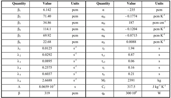
In Tables II and III the main input data pertaining severally to the reference BoC and EoC configurations are given (ERANOS-2.1, JEFF-3.1 data library calculations). Input parameters have been perturbed in order to investigate the
LP3.G2 - 14 - CERSE-POLIMI RL-1138/2010 open loop dynamic behaviour of DEMO core, as well as to observe and compare BoC and EoC new equilibrium configurations after the transients. In particular, the effects of lead inlet temperature increase (+ 10 K compared to its nominal value), and of an ideal control rod extraction (corresponding to a reactivity step of + 50 pcm) have been analyzed separately. Simulations have been started at initial time 1 s and run for 300 s, in order for the asymptotic output values to be reached.
TABLE II
DEMO core BoC reference data.
Quantity Value Units Quantity Value Units
β1 6.142 pcm α - 235 pcm β2 71.40 pcm αD - 0.1774 pcm K-1 β3 34.86 pcm αH 187 pcm cm-1 β4 114.1 pcm αL - 0.1204 pcm K-1 β5 69.92 pcm αR - 0.8715 pcm K-1 β6 22.68 pcm αZ 0.0088 pcm K-1 λ1 0.0125 s-1 τf 1.94 s λ 2 0.0292 s-1 τc1 0.87 s λ 3 0.0895 s-1 τc2 0.06 s λ 4 0.2575 s-1 τl 0.16 s λ 5 0.6037 s-1 τ0 0.21 s λ 6 2.6688 s-1 Mf 2391 kg Λ 8.0659·10-7 s C f 317.5 J kg-1 K-1 β 319 pcm q0 300·106 W TABLE III
DEMO core EoC reference data.
Quantity Value Units Quantity Value Units
β1 6.224 pcm α - 268 pcm β2 72.33 pcm αD - 0.2019 pcm K-1 β3 35.34 pcm αH 70 pcm cm-1 β4 115.5 pcm αL - 0.1408 pcm K-1 β5 70.75 pcm αR - 0.9234 pcm K-1 β6 22.89 pcm αZ - 0.1949 pcm K-1 λ1 0.0125 s-1 τf 1.99 s λ 2 0.0292 s-1 τc1 0.89 s λ 3 0.0895 s-1 τc2 0.06 s λ 4 0.2573 s-1 τl 0.16 s λ 5 0.6025 s-1 τ0 0.21 s λ 6 2.6661 s-1 Mf 2391 kg Λ 8.4980·10-7 s C f 317.5 J kg-1 K-1 β 323 pcm q0 300·106 W
LP3.G2 - 15 - CERSE-POLIMI RL-1138/2010
Lead Inlet Temperature Perturbation
The core inlet temperature has been enhanced by 10 K, leading to an insertion of negative reactivity (Fig. 3) due to both the instantaneous radial expansion and the lead density feedbacks, the latter being induced by the coolant average temperature increase (Fig. 4).
-12 -10 -8 -6 -4 -2 0 0 50 100 150 200 250 300 R ea cti vi ty [ pc m ] Time [s] BoC EoC
Fig. 3. Core reactivity variation following an enhancement by 10 K of core inlet temperature.
0 2 4 6 8 10 0 50 100 150 200 250 300 δTl [K ] Time [s] BoC EoC
Fig. 4. Lead average temperature variation following an enhancement by 10 K of core inlet temperature.
Because of the negative reactivity injection brought by higher lead temperatures, the core power undergoes a prompt decrease in the first part of the transient (Fig. 5), as far as the contribution of Doppler (due to the fuel average temperature reduction showed in Fig. 6) and axial expansion (due to the increased cladding temperature depicted in Fig. 7) start balancing the effects of lead temperature on reactivity at BoC.
The same general trend is observed also for the EoC situation, except for the opposite contribution of axial expansion to reactivity, which is negative. Indeed, only the Doppler effect is accountable for the reactivity raise after the peak of – 11 pcm (reached at time 0.5 s) caused by both higher coolant temperatures and core axial displacement.
Correspondingly, the reactivity increases again showing first a rapid rise and then a slower slope due to the opposing contribution of the axial contraction effect (at BoC), finally reinstating criticality.
LP3.G2 - 16 - CERSE-POLIMI RL-1138/2010
Therefore, the reactor power stabilizes to a new equilibrium value, approximately 22.4 and 22.1 MWth lower than the
nominal one at BoC and EoC, respectively.
-25 -20 -15 -10 -5 0 0 50 100 150 200 250 300 δq [ M W ] Time [s] BoC EoC
Fig. 5. Reactor power variation following an enhancement by 10 K of core inlet temperature.
-60 -50 -40 -30 -20 -10 0 0 50 100 150 200 250 300 δTf [K ] Time [s] BoC EoC
Fig. 6. Fuel average temperature variation following an enhancement by 10 K of core inlet temperature.
0 2 4 6 8 10 0 50 100 150 200 250 300 δTc [K ] Time [s] BoC EoC
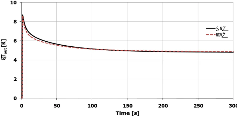
LP3.G2 - 17 - CERSE-POLIMI RL-1138/2010 At the end of the transient, the lead outlet temperature shows a positive variation (+ 4.80/+ 4.88 K at BoC/EoC), as Fig. 8 illustrates, but smaller than both the inlet perturbation and the average coolant temperature enhancement (+ 7.40/+ 7.44 K at BoC/EoC), due to the decrease in reactor power outlined in Fig. 5. On the contrary, the fuel temperature response is monotonically negative and settles at - 53.9/- 54.3 K respectively.
As to cladding temperature, after the peak of + 8.36/+ 8.24 in the very first part of the transient, it eventually sets at a relative variation of + 3.44/+ 3.54 with respect to the steady state value.
0 2 4 6 8 10 0 50 100 150 200 250 300 δTou t [K ] Time [s] BoC EoC
Fig. 8. Core outlet temperature variation following an enhancement by 10 K of core inlet temperature.
In order to verify the model prediction accuracy, the energy balance over the whole core has been calculated:
(
)
MWT T C
q=Γ l( out− in)=25757⋅145.6⋅484.80−410=280.51 (23)
for the BoC situation, whereas for EoC:
(
)
MWT T C
q=Γ l(out− in)=25757⋅145.6⋅ 484.88−410=280.81 (24)
Looking at the model results, the reactor thermal power (Fig. 5) after transient is found to be 277.6/277.9 MWth,
respectively, hence the error committed using a linearized model is almost negligible.
Control Rod Extraction
A further perturbation has been performed in order to evaluate DEMO dynamic response to a step reactivity insertion of 50 pcm (Fig. 9) at both BoC and EoC.
As Fig. 10 highlights, the expected response is observed, i.e. the initial, instantaneous power rise (prompt jump), whose
time characteristic (0.6/0.5 s at BoC/EoC) and huge amplitude (50/48 MWth at BoC/EoC) are essentially determined by
LP3.G2 - 18 - CERSE-POLIMI RL-1138/2010 0 10 20 30 40 50 60 0 50 100 150 200 250 300 R ea cti vi ty [ pc m ] Time [s] BoC EoC
Fig. 9. Core reactivity variation following an externally given perturbation of 50 pcm.
As Fig. 10 highlights, the expected response is observed, i.e. the initial, instantaneous power rise (prompt jump),
whose time characteristic (0.6/0.5 s at BoC/EoC) and huge amplitude (50/48 MWth at BoC/EoC) are essentially
determined by the prompt neutron life time and the delayed neutron fraction of the system.
0 20 40 60 80 100 0 50 100 150 200 250 300 δq [ M W] Time [s] BoC EoC
Fig. 10. Reactor power variation following a step reactivity insertion of 50 pcm.
After the power high peak at the transient beginning, fuel and lead temperatures (Figs. 11 and 12) start rising monotonically so as to balance the positive reactivity introduced by extracting the ideal control rod.
At BoC the considerable increase of cladding temperature, which finally settles at a relative variation of + 28.3 K (Fig. 13), opposes the corresponding negative reactivity feedbacks; the reactor power rises to a new stable value,
96.6 MWth higher than the nominal one. At EoC the negative feedback due to axial expansion combines to bring about
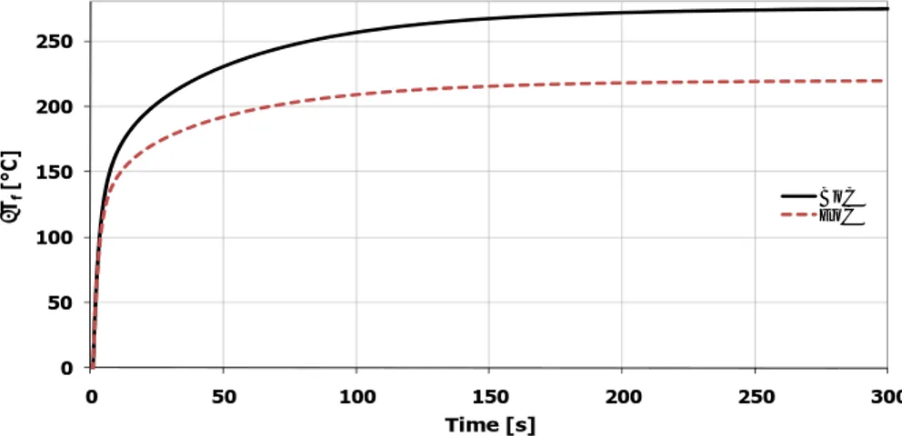
LP3.G2 - 19 - CERSE-POLIMI RL-1138/2010 0 50 100 150 200 250 0 50 100 150 200 250 300 δTf [° C] Time [s] BoC EoC
Fig. 11. Fuel average temperature variation following a step reactivity insertion of 50 pcm.
0 2 4 6 8 10 12 0 50 100 150 200 250 300 δTl [K ] Time [s] BoC EoC
Fig. 12. Lead average temperature variation following a step reactivity insertion of 50 pcm.
0 5 10 15 20 25 30 0 50 100 150 200 250 300 δTc [K ] Time [s] BoC EoC
Fig. 13. Cladding average temperature variation following a step reactivity insertion of 50 pcm.
At the end of the transient, the fuel temperature variation results significantly positive in turn, tending asymptotically to + 276/+ 220 K at BoC/EoC.
LP3.G2 - 20 - CERSE-POLIMI RL-1138/2010 As evident in Fig. 12, also the average coolant temperature features a positive variation of 11.2/8.8 K, and the lead outlet temperature shows an analogous trend but characterized by a major amplitude, resulting in a total enhancement of 22.4/17.5 K (Fig.14). 0 5 10 15 20 25 0 50 100 150 200 250 300 δTou t [K ] Time [s] BoC EoC
Fig. 14. Core outlet temperature variation following a step reactivity insertion of 50 pcm.
By applying the energy balance on the whole core at BoC:
(
)
MW T T C q=Γ l(out− in)=25757⋅145.6⋅502.4−400=384.0 (25) and EoC(
)
MW T T C q=Γ l(out− in)=25757⋅145.6⋅ 497.5−400=365.6 , (26)it has been observed that the model predictions overestimate the power transferred to coolant of about 12.6 and 9.9
MWth respectively, which have been judged as well acceptable results.
Analysis of the impact of not-linked axial expansion and average coolant temperature radial expansion
The reference model (22) has been modified so as to specifically allow the demonstration of the impact of different phenomena during BoC and EoC transients.
In particular, the reactivity feedback calculations have been modified to be based on the average fuel and coolant temperatures rather than cladding average and coolant inlet temperatures, respectively.
The first modification has been required to assess the impact of assuming the pellet column to be not-linked to the cladding –and consequently the axial expansion to be controlled by the fuel temperature, as expressed in Eq. (14); the latter has been applied in order to evaluate the effect of considering the core radial expansion to be driven by the coolant average temperature, pursuant to Eq. (15).
In ANNEX A the main input parameters and results pertaining to such analyses have been accounted for what concerns parameters subject to the most restricting technological constraints, namely fuel and superficial cladding temperatures.
LP3.G2 - 21 - CERSE-POLIMI RL-1138/2010 In the case of core inlet temperature enhancement, no significant differences from the reference simulations have been generally found. In particular, the fuel average temperature asymptotic variation has turned out to range from – 67 K (not-linked configuration, core inlet temperature radial expansion) to - 44 K (linked configuration, lead average temperature radial expansion) at BoC, and from – 45 K (linked configuration, core average temperature radial expansion) to - 24 K (not-linked configuration, lead average temperature radial expansion) at EoC.
The cladding average temperature excursion varies from a minimum of + 4.44 K (linked configuration, lead average temperature radial expansion) to a maximum of + 5.35 K (not-linked configuration, lead average temperature radial expansion) at BoC, and from a minimum of + 7.46 K (not-linked configuration, core inlet temperature radial expansion) to a maximum of + 7.78 K (linked configuration, lead average temperature radial expansion) at EoC, the corresponding reference values being + 3.44 K and + 3.54 K respectively.
As to power level, asymptotic variations from the steady-state values spread from – 18.3 MWth (not-linked
configuration, core inlet temperature radial expansion) to – 15.8 MWth (not-linked configuration, lead average
temperature radial expansion) at BoC, and from – 19.2 MWth (linked configuration, lead average temperature radial
expansion) to - 8.2 MWth (not-linked configuration, lead average temperature radial expansion) at EoC.
In the case of a step reactivity insertion of 50 pcm, the fuel average temperature asymptotic variation has turned out to range from + 230 K (linked configuration, lead average temperature radial expansion) to + 339 K (not-linked configuration, core inlet temperature radial expansion) at BoC, and from + 118 K (not-linked configuration, core average temperature radial expansion) to + 189 K (linked configuration, lead average temperature radial expansion) at EoC.
The cladding average temperature excursion varies from a minimum of + 20.1 K (not-linked configuration, lead average temperature radial expansion) to a maximum of + 23.6 K (linked configuration, lead average temperature radial expansion) at BoC, and from a minimum of + 8.2 K (not-linked configuration, lead average temperature radial expansion) to a maximum of + 19 K (linked configuration, lead average temperature radial expansion) at EoC, the corresponding reference values being + 28 K and + 22 K respectively.
As to power level, asymptotic variations from the steady-state values spread from + 68 MWth (not-linked configuration,
lead average temperature radial expansion) to + 80 MWth (not-linked configuration, core inlet temperature radial
expansion) at BoC, and from + 28 MWth (not-linked configuration, lead average temperature radial expansion) to + 65
MWth (linked configuration, lead average temperature radial expansion) at EoC, pointing a large variability out.
2.5 DEMO core open loop stability
Stability and natural response characteristics of the continuous-time LTI system (i.e., linear with matrices that are constant with respect to time) described in Eq. (22) have been also investigated directly by means of its representative transfer function, which has been obtained by Laplace-transforming the state-space model itself in MATLAB. The matrix-valued transfer function:
) ( ) ( ) ( s U s Y s G = (27)
LP3.G2 - 22 - CERSE-POLIMI RL-1138/2010 provides indeed qualitative insights into the response characteristics of the system, being stability very easy to infer from the related pole-zero plot: in order for a linear system to be stable, in fact, all of its poles (namely, roots of the characteristic equation or, equivalently, eigenvalues of the matrix ) must have negative real parts, that is they must all lie within the left-half of the s-plane [19].
TABLE IV Pole location.
Pole Value at BoC [s-1] Value at EoC [s-1]
P1 - 0.0188 - 0.0120 P2 - 0.0201 - 0.0214 P3 - 0.0785 - 0.0801 P4 - 0.199 - 0.208 P5 - 0.561 + 0.125i - 0.580 + 0.136i P6 - 0.561 - 0.125i - 0.580 - 0.136i P7 - 2.48 - 2.47 P8 - 6.58 - 6.54 P9 - 27.1 - 27.0 P10 -3.96·103 -3.80·103
As a result of such an investigation, the system has been confirmed to be stable at both BoC and EoC, since all its ten
poles have strictly negative real part, the dominant ones being at - 0.0188 and - 0.0120 s-1, respectively (see Table IV).
3
NEUTRON KINETICS EVALUATIONSTo extend the previous DEMO neutronics analyses by investigating core responses to transient initiators such as temperature changes or control rod shifts, a preliminary study of DEMO core kinetics has been carried out. Indeed, kinetics studies are fundamental not only to predict the reactor behaviour under operational conditions, but also to evaluate consequences of hypothetical accidents for safety purposes.
In this context, the ERANOS KIN3D module [10] has been employed to accomplish simulations of reactor transients induced by both fuel temperature (Doppler effect) and coolant temperature (coolant density effect) variations, and a FAR complete withdrawal and insertion.
To perform such analyses, the perturbations related to the reactivity effects under investigation have been simulated by cross-section changes in some reactor sub-regions, based on the outcomes of the previous study of DEMO core dynamics concerning fuel and coolant temperature variations following a stepwise reactivity insertion of 50 pcm and an increase of the coolant inlet temperature of 10 K. Material density and temperature distributions obtained from the previous coupled point-kinetics and thermal-hydraulics model have been employed to compute effective neutron cross-sections for reactor sub-regions that have been used as input data for the present core neutronics calculations.
Reactivity coefficients and kinetics parameters, such as βeff, have been calculated accordingly by employing the
perturbation theory formalism for the steady-state conditions, in order to assess both reactivity global variations and their breakdown into the most relevant nuclide contributions.
LP3.G2 - 23 - CERSE-POLIMI RL-1138/2010 KIN3D point and direct space-time kinetics solution schemes have been finally analyzed and compared, with the purpose to test the code capabilities in view of more complex transient evaluations to be performed in the future.
3.1 Computational schemes
Multi-group cross-sections associated to every reactor zone have been processed by means of ECCO and tri-dimensional core models have been set up. The whole system has then been solved through both the variational nodal (transport and diffusion options) and finite-difference (diffusion) methods, in order to evaluate their impact on the solution accuracy. For the same purpose, nodal transport calculations have been performed using either spherical
harmonics (PN) and simplified spherical harmonics (SPN), while representing the scattering cross-sections with the P0
and P1 Legendre polynomial expansion (P3P0, P3P1, SP3P0, SP3P1 respectively).
Regarding KIN3D, the module solves the time-dependent neutron transport equation and performs perturbation calculations. The treatment of the time dependence is based on two main models: point and space-time kinetics.
In point kinetics, the flux shape (that determines the power shape and reactivity coefficients) is assumed to be constant during the transient, the reactor being considered to be in steady state mode for t < 0, and being t = 0 the beginning of a transient.
Concerning the space-time kinetics calculations, the time-dependent problem is transformed into a sequence of steady-state-like problems, solved by VARIANT every time step, whereas cross-sections are assumed to be known at certain times during the transient (e.g. FAR position at initial and final state), and an interpolation between these time points is performed. Two main space-time kinetics methods have been tested: the direct method and the quasi-static space-time factorisation scheme.
The first uses a straightforward time discretization of the time-dependent neutron transport (or diffusion) equation, featuring a relative simplicity –since there is no need for perturbation theory calculations which require computation of the adjoint steady-state flux-, but a quite relevant computing cost, as it has been found that the method requires extremely fine time steps for transient simulations in fast reactors due to considerably small values of the mean
generation time (Λ ~ 8.2·10-7 s, DEMO BoC reference calculations).
The second is based on the observation that the flux shape does not have to be updated as frequently as the flux amplitude, which represents a rapidly varying factor that is calculated with small time steps by employing the point kinetics integration scheme. Flux shape updates provide new power distributions and new sets of reactivity coefficients, showing good performances without any significant loss of accuracy. The equations, however, are more complicated than those of the direct method, adjoint and perturbation theory calculations being necessary.
3.2 Results
KIN3D has been employed to perform simulations of DEMO core transients induced by fuel and coolant temperature variations, and FAR complete withdrawal and insertion.
Consistently with the final steady-state temperature distributions resulting from the dynamics simulations performed, where the transients originated from a stepwise reactivity insertion of 50 pcm and an increase of the coolant inlet temperature of 10 K, deviations from the nominal parameters have been applied as follows:
LP3.G2 - 24 - CERSE-POLIMI RL-1138/2010 - fuel temperature reduction (variation: - 54 K);
- coolant density reduction (maximum variation: - 0.13 %).
In point-kinetics calculations, the respective perturbations have been introduced at time 0 ≤ t ≤ 76 s, and simulations were run for 500 s with a time step ∆t = 0.5 s for 0 ≤ t ≤ 100 s, and ∆t = 5 s from for 100 ≤ t ≤ 500 s.
Furthermore, one of the 16 regulation FARs (uniformly inserted to half active height at BoC) has been simulated to be
either completely extracted from the core or totally pulled down, by figuring a speed of approximately 0.3 m s-1.
Perturbations have been introduced at time t = 1 s, and simulations were run for 10 s with a time step ∆t = 0.01 s for 0 ≤ t ≤ 1.5 s, and ∆t = 0.1 s for 1.5 ≤ t ≤ 10 s.
Fuel temperature variation
The calculated KIN3D reactivity variation due to an increase of 276 K in the fuel average temperature has turned out to
be of the order of -50 pcm, showing a very good agreement (1.8 % discrepancy on ∆ρ) with the direct P3P0 transport
calculations performed in (§ 2).
As shown in Fig. 15, a perfect accordance (0.06 % discrepancy) has been found also between SP3P0 transport and
diffusion calculations, whose results are ∆ρ = - 49.75 pcm and ∆ρ = - 49.78 pcm respectively, despite a 600 pcm
maximum discrepancy on the corresponding absolute values of keff. Indeed, systematic errors in over-estimating or
under-estimating keff actual values occur both in the reference and in the perturbed calculations, and differentials result
less sensitive to numerical schemes as consequence of such ‘first order’ compensations.
Similarly, a reactivity increase (∆ρ = + 10.9 pcm) has been induced by a 54 K reduction of the fuel average temperature. This smaller effect has been consistently determined in diffusion and transport calculations, the obtained results differing by only 0.06 %. -60 -50 -40 -30 -20 -10 0 10 20 0 10 20 30 40 50 60 70 80 90 100 R e act iv it y va ri at io n [ p cm ] Time [s] diffusion (+ 276 K) transport (+ 276 K) normalized diffusion (+ 276 K) diffusion (- 54 K) transport (- 54 K) normalized diffusion (- 54 K)
Fig. 15. Reactivity variations due to fuel temperature changes (KIN3D point-kinetics calculations).
Satisfactory results have been achieved with regard to the amplitude function curves as well: as depicted in Fig. 16, the exponentially soaring and dimming-to-zero trends refer to the positive and negative reactivity insertions, respectively.
Negligible disagreements between SP3P0 transport and diffusion calculations have been obtained, the maximum gap
turning out to be of the order of 0.4 %.
Point-kinetics results have been then compared to the reference space-time direct results, and a 2 % discrepancy on the amplitude function has been found.
LP3.G2 - 25 - CERSE-POLIMI RL-1138/2010 0,00 1,00 2,00 3,00 4,00 5,00 6,00 0 100 200 300 400 500 A m p li tu d e fu n c ti o n [-] Time [s] diffusion (+ 276 K) transport (+ 276 K) normalized diffusion (+ 276 K) diffusion (- 54 K) transport (- 54 K) normalized diffusion (- 54 K)
Fig. 16. Amplitude functions following fuel temperature changes (KIN3D point-kinetics calculations).
In order to test the KIN3D quasi-static space-time factorization scheme, a shorter transient has been simulated, due to the need of reducing the time step to make it comparable to the mean generation time. The resulting reactivity and amplitude have been compared to the point-kinetics results: a 0.7 % and 0.2 % discrepancy has been found for the respective figures. Additionally, the reactivity effect for the reference scenario (+ 276 K fuel temperature variation) has been decomposed reaction-wise, isotope-wise, and energy-group-wise, the breakdown being performed by means of the ERANOS PERTURBATION modules.
As summarized in Tab. V, the reaction-wise decomposition has shown that the dominant negative effect is due to
capture, whereas fission gives a positive contribution. More specifically, the 238U increased captures are responsible up
to 91% of the total reactivity decrease; a negative effect is also due to 240Pu and 239Pu capture, but the strong
compensation between the latter’s capture and fission ends up with a slight positive net contribution.
First-order perturbation calculations (employing direct and adjoint finite-difference diffusion fluxes) have turned out to be in good agreement with KIN3D (variational nodal diffusion and transport) results concerning the global reactivity effect, which has been satisfactorily assessed with a 0.9 % discrepancy.
TABLE V
Doppler reactivity effect breaking-down by nuclides and reactions.
Isotope Capture Fission Leakage Elastic
Removal Inelastic Removal n,xn Removal TOTAL Cr53 0.00 0.00 0.00 -0.01 0.00 0.00 -0.01 Fe56 -0.27 0.00 0.00 -0.03 0.00 0.00 -0.30 Mo96 0.01 0.00 0.00 0.00 0.00 0.00 0.01 Pb204 -0.01 0.00 0.00 0.00 0.00 0.00 -0.01 Pb206 -0.03 0.00 0.00 -0.01 0.00 0.00 -0.03 Pb207 -0.06 0.00 0.00 -0.01 0.00 0.00 -0.07 Pb208 0.00 0.00 0.00 -0.02 0.00 0.00 -0.02 U238 -45.73 0.01 0.32 0.05 -0.10 0.00 -45.46 Pu238 -0.03 -0.03 0.00 0.00 0.00 0.00 -0.06 Pu239 -5.53 7.52 -0.11 0.00 0.00 0.00 1.87
LP3.G2 - 26 - CERSE-POLIMI RL-1138/2010 Pu240 -4.14 0.45 -0.06 0.00 0.00 0.00 -3.75 Pu241 0.03 -1.54 -0.01 0.00 0.00 0.00 -1.51 Pu242 -0.25 0.00 -0.01 0.00 0.00 0.00 -0.25 B10 -0.50 0.00 0.00 0.00 0.00 0.00 -0.50 O16 0.00 0.00 0.00 -0.12 0.00 0.00 -0.12 TOTAL -56.50 6.41 0.14 -0.15 -0.10 0.00 -50.20
Coolant density variation
The calculated KIN3D reactivity variation due to an increase of 11 K in the coolant average temperature has turned out to be of the order of - 16 pcm. As shown in Fig. 17, a fairly good agreement (5.6 % discrepancy) has been found
between SP3P0 transport and diffusion calculations, whose results are ∆ρ = + 16.05 pcm and ∆ρ = +15.14 pcm
respectively. -18 -16 -14 -12 -10 -8 -6 -4 -2 0 0 10 20 30 40 50 60 70 80 90 100 R e ac ti vi ty va ri a ti on [ p cm ] Time [s] diffusion transport normalized diffusion
Fig. 17. Reactivity variations due to coolant temperature increase by 11 K (KIN3D point-kinetics calculations).
Quite reasonable accordance has been achieved in determining the respective amplitude functions: as depicted in Fig.
18 in fact, the diffusion exponential dimming-to-zero trends show a 11 % disagreement with respect to the SP3P0
transport outcome. 0,00 0,20 0,40 0,60 0,80 1,00 1,20 0 100 200 300 400 500 A m pl it ud e f u nc ti on [ -] Time [s] diffusion transport normalized diffusion
LP3.G2 - 27 - CERSE-POLIMI RL-1138/2010 As in the Doppler effect case, the global reactivity variation has been broken down reaction-wise, isotope-wise, and energy-group-wise. First-order perturbation calculations have turned out to be in fair agreement with KIN3D results concerning the global reactivity effect, which has been assessed with a 13 % discrepancy.
As summarized in Tab. VI, the reaction-wise decomposition has shown that the negative effect is mostly due to leakage, which accounts for about - 23 pcm and, as expected, is almost entirely due to the lead, whereas capture, elastic and inelastic removals oppose the reactivity diminution.
Regarding the fuel most relevant nuclides, 238U has confirmed to contribute positively since even-even isotope capture
cross-sections decrease, due to the spectral hardening following a coolant density reduction.
Absolute values of keff have been finally determined with approximately 60 pcm difference between P3P0 and SP3P0
transport methods, and with approximately 550 pcm gap between SP3P0 transport and diffusion calculations.
TABLE VI
Doppler reactivity effect breaking-down by nuclides and reactions.
Isotope Capture Fission Leakage Elastic
Removal Inelastic Removal n,xn Removal TOTAL C0 0.00 0.00 -0.01 0.00 0.00 0.00 -0.01 Cr52 0.00 0.00 -0.02 0.01 0.00 0.00 -0.01 Fe56 0.11 0.00 -0.25 0.11 0.01 0.00 -0.02 Mo95 0.01 0.00 0.00 0.00 0.00 0.00 0.01 U238 0.19 -0.03 -0.02 0.00 0.03 0.00 0.18 Pu239 0.03 -0.12 0.00 0.00 0.00 0.00 -0.09 Pu240 0.02 -0.01 0.00 0.00 0.00 0.00 0.01 Pu241 0.00 -0.01 0.00 0.00 0.00 0.00 -0.01 B10 -0.13 0.00 -0.01 0.00 0.00 0.00 -0.14 B11 0.00 0.00 -0.02 0.00 0.00 0.00 -0.01 O16 0.00 0.00 -0.04 0.06 0.00 0.00 0.02 Pb204 0.40 0.00 -0.36 0.05 0.14 0.00 0.23 Pb206 0.93 0.00 -5.18 0.67 2.05 -0.01 -1.53 Pb207 0.59 0.00 -5.10 0.78 1.46 -0.03 -2.31 Pb208 0.16 0.00 -11.96 1.46 0.92 -0.05 -9.47 TOTAL 2.33 -0.16 -22.98 3.14 4.62 -0.09 -13.15
Control element shifting
KIN3D has been finally employed to simulate a transient initiated by either a FAR complete extraction or its total insertion from/into the core.
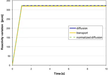
The corresponding reactivity variations have turned out to be of the order of ∆ρ = + 320 pcm (see Fig. 19) and ∆ρ = - 550 pcm, the latter effect being greater because of the weaker self-shielding in the bottom part of the active core.
A very good agreement (1.2 % and 0.5 % discrepancies) has been found also between SP3P0 transport and diffusion
calculations, resulting respectively in ∆ρ = + 318 pcm and ∆ρ = + 322 pcm in the case of rod withdrawal, and in ∆ρ = - 554 pcm and ∆ρ = - 552 pcm in the case of rod insertion.
LP3.G2 - 28 - CERSE-POLIMI RL-1138/2010 As in the previous cases, the global reactivity variation following the reference perturbation (i.e. FAR complete extraction) has been decomposed into its main contributors (see Tab. VII) by applying the first-order perturbation theory. Results have turned out to be in fair agreement with KIN3D results concerning the global reactivity effect, which has been assessed with a 14 % maximum discrepancy.
The reaction-wise decomposition has shown that the positive effect is predominantly due to the significant reduction of
captures in the FA deprived of absorbers, accounting for about 354 pcm, 350 of which are due to 10B; a minor positive
contribution (+ 30 pcm) is also due to 10B and 11B elastic removal.
0 50 100 150 200 250 300 350 0 2 4 6 8 10 R eac ti vi ty v a ri at ion [ p cm ] Time [s] diffusion transport normalized diffusion
Fig. 19. Reactivity variation due to a FAR complete withdrawal from the active core (KIN3D point-kinetics calculations).
TABLE VI
FAR withdrawal reactivity effect breaking-down by nuclides and reactions.
Isotope Capture Fission Transport Elastic
Removal Inelastic Removal n,xn Removal TOTAL C0 -0,01 0,00 0,78 -2,05 -0,01 0,00 -1,29 Si28 0,00 0,00 0,00 0,00 0,00 0,00 0,01 Cr52 0,00 0,00 0,03 0,01 0,00 0,00 0,05 Cr50 0,00 0,00 0,00 0,01 0,00 0,00 0,01 Cr53 0,00 0,00 0,01 0,01 0,00 0,00 0,02 Mn55 0,00 0,00 0,00 0,00 0,00 0,00 0,01 Fe54 0,01 0,00 0,03 0,01 0,00 0,00 0,05 Fe56 0,11 0,00 0,12 0,19 0,02 0,00 0,45 Fe57 0,00 0,00 0,02 0,00 0,00 0,00 0,02 U235 0,01 -0,13 0,00 0,00 0,00 0,00 -0,11 U238 2,23 -0,70 -1,33 0,07 0,66 -0,01 0,92 Pu238 0,03 -0,28 -0,01 0,00 0,00 0,00 -0,26 Pu239 0,78 -10,03 -0,31 0,01 0,08 0,00 -9,47 Pu240 0,41 -1,09 -0,16 0,01 0,05 0,00 -0,78 Pu241 0,09 -1,50 -0,03 0,00 0,01 0,00 -1,44 Pu242 0,11 -0,21 -0,05 0,00 0,02 0,00 -0,12
LP3.G2 - 29 - CERSE-POLIMI RL-1138/2010 Pb204 0,03 0,00 -0,07 0,01 0,01 0,00 -0,02 Pb206 0,06 0,00 -1,04 0,08 0,22 0,00 -0,69 Pb207 0,05 0,00 -1,04 0,08 0,15 0,00 -0,75 Pb208 0,02 0,00 -2,49 0,15 0,08 0,00 -2,24 Ar40 0,00 0,00 0,02 -0,01 0,00 0,00 0,01 O16 0,03 0,00 -1,59 1,48 0,00 0,00 -0,07 B10 350,49 0,00 -3,62 12,21 0,10 0,00 359,18 B11 0,01 0,00 -4,12 18,35 0,10 0,00 14,34 TOTAL 354,47 -13,94 -14,82 30,63 1,51 -0,02 357,83
4
PRELIMINARY EVALUATIONS OF CORE MECHANICS-
RELATED ASPECTSThe need of approaching mechanics-related aspects has led to an alternative and more simplified dynamic model of DEMO core. As in (§ 2), the primary system has been assumed to consist only in the active core, disregarding both upper and lower plena, and a single average channel representation has been adopted.
Reactor power has been described by neutron point-kinetics equations with six delayed neutron precursor groups. An energy balance over the fuel pin surrounded by coolant -in which reactor power is an input retrieved from reactor kinetics- has been employed to determine the fuel and the lead temperature behaviour.
System expansions and contractions have been simulated under the simplifying hypothesis of considering a cylindrical-shape core, whose relative displacement vary instantaneously with temperature.
The so-calculated thermal-hydraulic and spatial parameters have been finally employed to insert the reactivity feedbacks into the neutronics equations (Fig. 20).
H Ψ Ci CORE Tf Tl V Tin δρ(t) δψ(t) δq(t) δTf(t) δTl(t) δTin(t) δTout(t) δTin(t) δH(t) δTf(t) δTl(t) δρ(t) δH(t) δTf(t) δV(t)/V δTl(t) Kinetics Thermal-hydraulics Mechanics Reactivity Input Tout