Complex Movements for Voluntary Actions Evoked by Electrical Stimulation in the Motor Cortex of Rats

Università degli Studi di Ferrara

DOTTORATO DI RICERCA IN

SCIENZE BIOMEDICHE

CICLO XXIV

COORDINATORE Prof. Capitani Silvano

Complex Movements for Voluntary Actions Evoked by

Electrical Stimulation in the Motor Cortex of Rats

Settore Scientifico Disciplinare BIO/09

Dottorando Tutore

Dott. Bonazzi Laura Dott. Franchi Gianfranco

______________________ ______________________

ÂfÉÇÉ Äx ávxÄàx v{x ytvv|tÅÉ

v{x w|ÅÉáàÜtÇÉ ÖâxÄ v{x á|tÅÉ äxÜtÅxÇàx?

ÅÉÄàÉ Ñ|∞ wxÄÄx ÇÉáàÜx vtÑtv|àõÊ

Index

1. Introduction

1.1 Rat motor cortex ………... pag. 7

1.2 Qualisys Optical Motion Capture System ………... pag. 9 1.3 Qualisys Track Manager (QTM) ………. pag. 10 1.4 Multivariate statistics ……… pag. 11 1.5 Tukey's test ……… pag. 14

2. Materials and Methods

2.1 Long-duration Intracortical Microstimulation ……….. pag. 18 2.2 Evoked movements characterization and map construction ……… pag. 19 2.3 Kinematic recording of complex movements and analysis ……… pag. 20 2.4 Data Presentation and Statistical Analysis ………. pag. 23

3. Results

3.1 Stimulation-evoked limb (wrist marker) movements ……… pag.26 3.2 Limb (wrist marker) movements kinematics ………. pag. 28 3.3 Stimulation-evoked paw (digit marker) movements ……….. pag. 29 3.4 Paw (digit marker) movement kinematics ………. pag. 30 3.5 Relation between limb and paw movement ……… pag. 31

4. Discussion

4.1 Methodological and Technical remarks ………. pag. 32 4.2 Why long-duration ICMS of the forelimb motor cortex evoked patterns

of coordinated movement ………... pag. 38

5. Figures ……… pag. 42

1. Introduction

Electrical intracortical microstimulation (ICMS) has been widely used to study the functional organization of the motor cortex. The ICMS carried out at low level of current with brief trains of electrical pulses (less than 60 ms: short-duration ICMS) have been used to characterize the topographic map of the body in mammal’s motor cortex (Asanuma et al., 1976; Donoghue and Wise, 1982). It has been suggested that the body maps in motor cortex attainable through short-duration ICMS was not exhaustive to characterize the complex aspect of the cortical motor control on voluntary movement (Schieber, 2001). Indeed, muscles twitches evoked by short-duration ICMS revealed the strength of synaptic link between cortical neurons and spinal motoneurons, but did cast no light on how motor cortex controlled the activation of spinal motoneurons during natural movement.

The ICMS with longer stimulus trains of about 500 ms (long-duration ICMS) evoked complex and coordinated movement, similar to those of natural behaviour (Graziano et al., 2002). Studies employing long-duration ICMS (Graziano et al., 2002 and 2005) provided evidence that the primate’s motor cortex contains in addition to the map of the body, a map of motor repertoire and a map of target locations for the animal hand in the extrinsic space. These maps could span the entire surface of the motor cortex, including primary motor (M1) and premotor areas and could develop overlapped in the same cortical region.

Whether the organizing features of cortical motor control described in primate were consistent across mammals were not completely explored. A previous study in rat (Haiss and Schwarz, 2005) provided evidence that different patterns of motor control are spatially separated and integrated into the whisker motor map suggesting that cortical separation was due to the specific drive of subcortical structures needed to generate different patterns of movement. A recent paper (Ramanathan et al., 2006) have reported that long-duration ICMS in rat motor cortex can result in complex, multijoint forelimb movements organized in a roughly topography. However, since this

study did not examined in detail the topography of evoked movements as it did not provide kinematic informations on evoked movements, it is worthy of interest to define quantitatively the patterns of forelimb movement evoked by long-duration ICMS. The quantitative approach make it possible to verify whether a topography of patterns of movement and a map of target location in space for the limb, can be highlighted in the rat motor cortex.

Guided by these considerations, we pose the question if different features of motor control (e.g. body map, movement patterns, target location in space) can develop overlapping maps in the forelimb region of the rat’s M1. We performed long-duration ICMS to evoke complex, multijoint forelimb movements and we used motion analysis tools to measure kinematic variables of electrically-evoked movements.

1.1 Rat motor cortex

In mammals, the hierarchical organization among the cortical motor areas is under investigation. The primary motor cortex (M1) was identified based on its agranular cytoarchitectonic (Brecht et al., 2004). The division between M1 and premotor cortex is notoriously fuzzy: it may be more of a gradient than a border (Graziano et al., 2002). Premotor cortex projects to and controls M1, which in turn projects to and controls the spinal cord. Damage to M1 does not cause a general loss of the ability to move; instead, it results in a specific deficit in fine manual coordination. Many new motor areas have been described, including the supplementary motor area, the cingulated motor areas and many subdivisions of the premotor cortex. However, M1 is the most important region for movement control. It contains a somatotopic representation of the major subdivisions of the body musculature and predominantly controls the limb muscles on the contralateral side of the body albeit only at the level of head, limbs and trunk. Within representations of body parts, M1 map appears to be organized in mostly distributed and overlapping patches (Schieber, 2001). The cortical map of movements is thought to be an emergent property of distributed, horizontal, modifiable network within the cortex (Donoghue, 1995).

In the rat primary motor cortex, the location of major subdivisions, such as the forelimb or hindlimb areas, is somatotopic and is consistent from animal to animal, but the internal organization of the pattern of movements represented within major subdivisions varies significantly between animals. The rat motor cortex includes both agranular primary motor cortex (AgL) and, in addition, a significant amount of the bordering granular somatic sensory cortex (Gr(SI)), as well as the rostral portion of the taste sensory insular or claustrocortex (Cl). The rat frontal cortex also contains a second, rostral motor representation of the forelimb, trunk and hindlimb (see figure below), which is somatotopically organized and may be the rat's supplementary motor area.

6 4 2 B -2 -4 -6 -2 -6 Hinlimb-4 Trunk Forelimb Eyes 6 4 2 B -2 -4 -6 -2 -6 Hinlimb-4 Trunk Forelimb Eyes

Both of these motor representations give rise to direct corticospinal projections (Neafsey et al., 1985), some of which may make monosynaptic connections with cervical enlargement motorneurons. Medial to the primary motor cortex, in cytoarchitectonic field AgM, is what appears to be part of the rat's frontal eye fields, a region which also includes the vibrissae motor representation. The somatic motor cortical output organization pattern in the rat is remarkably similar to that seen in the primate, whose primary, supplementary and frontal eye field cortical motor regions have been extensively studied.

1.2 Qualisys Optical Motion Capture System

Qualisys Optical Motion Capture is a system developed in Sweden since 1989 and today accepted all over the world. It enables the capture of motion that would be difficult to measure in other ways and it is used in medical and industrial applications. The Qualisys System uses high speed digital cameras (Qualisys ProReflex cameras, see figure below), to precisely capture the motion of a measurement object, with passive or active markers attached. These cameras (complied with the FDA CFR 1040.10 Class I classification) use short but quite strong infrared flashes to illuminate the markers. The flash is generated by LEDs on the front of the cameras. The technology is precise and delivers high quality data to the observer in real-time. The measurement system consists also of high advanced software (QTM) for tracking and analysis of motion data. Software tools perform basic motion calculations such as speed, acceleration, rotations and angles.

1.3 Qualisys Track Manager (QTM)

Qualisys Track Manager is a Windows-based data acquisition software with an interface that allows the user to perform 2D and 3D motion capture. Together with the Qualisys line of optical measurement hardware, QTM streamlines the coordination of all features in a sophisticated motion capture system and provide the possibility of rapid production of distinct and accurate 2D, 3D and 6D data. During the capture, real time 2D, 3D and 6D camera information is displayed allowing instant confirmation of accurate data acquisition. The individual 2D camera data is quickly processed and converted into 3D or 6D data by advanced algorithms, which are adaptable to different movement characteristics. The data can then be exported to analysis software via several external formats.

1.4 Multivariate statistics

Multivariate statistics is a form of statistics encompassing the simultaneous observation and analysis of more than one statistical variable. The application of multivariate statistics is multivariate analysis. Methods of bivariate statistics, for example simple linear regression and correlation, are special cases of multivariate statistics in which 2 variables are involved. Multivariate statistics concerns understanding the different aims and background of each of the different forms of multivariate analysis, and how they relate to each other. The practical implementation of multivariate statistics to a particular problem may involve several types of univariate and multivariate analysis in order to understand the relationships between variables and their relevance to the actual problem being studied. In addition, multivariate statistics is concerned with multivariate probability distributions, in terms of both:

 how these can be used to represent the distributions of observed data;

 how they can be used as part of statistical inference, particularly where several different quantities are of interest to the same analysis.

There are many different models, each with its own type of analysis:

1. Multivariate analysis of variance (MANOVA) extends the analysis of variance to cover cases where there is more than one dependent variable to be analyzed simultaneously: see also MANCOVA;

2. Multivariate regression analysis attempts to determine a formula that can describe how elements in a vector of variables respond simultaneously to changes in others. For linear relations, regression analyses here are based on forms of the general linear model;

3. Principal components analysis (PCA) creates a new set of orthogonal variables that contain the same information as the original set. It rotates the axes of variation to give a new set of orthogonal axes, ordered so that they summarize decreasing proportions of the variation;

4. Factor analysis is similar to PCA but allows the user to extract a specified number of synthetic variables, fewer than the original set, leaving the remaining unexplained variation as error. The extracted variables are known as latent variables or factors; each one may be supposed to account for covariation in a group of observed variables;

5. Canonical correlation analysis finds linear relationships among 2 sets of variables; it is the generalised (canonical) version of bivariate correlation;

6. Redundancy analysis is similar to canonical correlation analysis but allows the user to derive a specified number of synthetic variables from one set of (independent) variables that explain as much variance as possible in another (independent) set. It is a multivariate analogue of regression;

7. Correspondence analysis (CA), or reciprocal averaging, finds (like PCA) a set of synthetic variables that summarise the original set. The underlying model assumes chi-squared dissimilarities among records (cases). There is also canonical (or "constrained") correspondence analysis (CCA) for summarising the joint variation in 2 sets of variables (like canonical correlation analysis);

8. Multidimensional scaling comprises various algorithms to determine a set of synthetic variables that best represent the pairwise distances between records. The original method is principal coordinates analysis (based on PCA);

9. Discriminant analysis, or canonical variate analysis, is a statistical analysis to predict a categorical dependent variable by one or more continuous or binary independent variables and it is useful in determining whether a set of variables is effective in predicting category membership;

10. Linear discriminant analysis (LDA) computes a linear predictor from 2 sets of normally distributed data to allow for classification of new observations;

11. Clustering systems assign objects into groups (clusters) so that objects (cases) from the same cluster are more similar to each other than objects from different clusters;

12. Recursive partitioning creates a decision tree that attempts to correctly classify members of the population based on a dichotomous dependent variable;

13. Artificial neural networks extend regression and clustering methods to non-linear multivariate models.

There is a set of probability distributions used in multivariate analyses that play a similar role to the corresponding set of distributions that are used in univariate analysis when the normal distribution is appropriate to a dataset. These multivariate distributions are:

 Multivariate normal distribution;

 Wishart distribution;

1.5 Tukey's test

Tukey's test, also known as the Tukey range test, Tukey method, Tukey's honest significance test, Tukey's HSD test (Honestly Significant Difference test) (Lowry, 2008), or the Tukey–Kramer method, is a single-step multiple comparison procedure and statistical test generally used in conjunction with an ANOVA to find which means are significantly different from one another. Named after John Tukey, it compares all possible pairs of means, and is based on a studentized range distribution q (this distribution is similar to the distribution of t from the t-test) (Linton et al., 2007). The test compares the means of every treatment to the means of every other treatment; that is,

it applies simultaneously to the set of all pairwise comparisons μi - μj and identifies where the

difference between 2 means is greater than the standard error would be expected to allow. The confidence coefficient for the set, when all sample sizes are equal, is exactly 1 − α. For unequal sample sizes, the confidence coefficient is greater than 1 − α. In other words, the Tukey method is conservative when there are unequal sample sizes. Tukey's test is based on a formula very similar to that of the t-test. In fact, Tukey's test is essentially a t-test, except that it corrects for experiment-wise error rate (when there are multiple comparisons being made, the probability of making a type I error increases. Tukey's test corrects for that, and is thus more suitable for multiple comparisons than doing a number of t-tests would be) (Linton et al., 2007).

The formula for Tukey's test is:

where YA is the larger of the 2 means being compared, YB is the smaller of the 2 means being

compared, and SE is the standard error of the data in question.

This qs value can then be compared to a q value from the studentized range distribution. If the qs

significantly different. Since the null hypothesis for Tukey's test states that all means being compared are from the same population (i.e. μ1 = μ2 = μ3 = ... = μn), the means should be normally

distributed (according to the central limit theorem). This gives rise to the normality assumption of Tukey's test. The Tukey confidence limits for all pairwise comparisons with confidence coefficient of at least 1 − α are:

Notice that the point estimator and the estimated variance are the same as those for a single pairwise comparison. The only difference between the confidence limits for simultaneous comparisons and those for a single comparison is the multiple of the estimated standard deviation. Also note that the sample sizes must be equal when using the studentized range approach.

is the standard deviation of the entire design, not just that of the 2 groups being compared. The Tukey–Kramer method for unequal sample sizes is as follows:

where n i and n j are the sizes of groups i and j respectively. The degrees of freedom for the whole

design is also applied.

Tukey's test is based on the comparison of 2 samples from the same population. From the first sample, the range (calculated by subtracting the smallest observation from the largest, or range = maxi (Yi) – mini (Yi) where Yi represents all of the observations) is calculated, and from the second

sample, the standard deviation is calculated. The studentized range ratio is then calculated:

where q = studentized range, and s = standard deviation of the second sample. This value of q is the basis of the critical value of q, based on 3 factors:

1. α (the type I error rate, or the probability of rejecting a true null hypothesis); 2. n (the number of degrees of freedom in the first sample (the one from which

range was calculated);

3. v (the number of degrees of freedom in the second sample (the one from which s was calculated);

The distribution of q has been tabulated and appears in many textbooks on statistics.

If there are a set of means (A, B, C, D), which can be ranked in the order A > B > C > D, not all possible comparisons need be tested using Tukey's test. To avoid redundancy, one starts by

comparing the largest mean (A) with the smallest mean (D). If the qs value for the comparison of

means A and D is less than the q value from the distribution, the null hypothesis is not rejected, and the means are said have no statistically significant difference between them. Since there is no difference between the 2 means that have the largest difference, comparing any 2 means that have a smaller difference is assured to yield the same conclusion (if sample sizes are identical). As a result, no other comparisons need to be made (Linton et al., 2007).

Overall, it is important when employing Tukey's test to always start by comparing the largest mean to the smallest mean, and then the largest mean with the next smallest, etc., until the largest mean has been compared to all other means (or until no difference is found). After this, compare the second largest mean with the smallest mean, and then the next smallest, and so on. Once again, if 2 means are found to have no statistically significant difference, do not compare any of the means

between them (Linton et al., 2007). If only pairwise comparisons are to be made, the Tukey–Kramer

method will result in a narrower confidence limit (which is preferable and more powerful) than Scheffé' method.

2. Materials and Methods

A total of 7 male Albino rats, weighing 280-330 g were used to characterize the forelimb movement evoked by a long-duration intracortical stimulation (ICMS) and to perform a quantitative analysis of kinematics of these complex movements. Other 7 animals were used in pilot studies whose data were not included in the paper. The experimental plan was designed in compliance with Italian Law regarding the care and use of experimental animals (DL116/92) and approved by the institutional review board of the University of Ferrara and by the Italian Ministry of Health. For all experimental procedures rats were anesthetized initially with ketamine HCl (80 mg/Kg i.p.). For the duration of the experiment, anesthesia was maintained by supplementary ketamine injections (4 mg/Kg i.m given as required, typically every 25-30 minutes) so as to achieve long-latency and sluggish hindlimb withdrawal upon pinching the hindfoot. Under anesthesia, the body temperature was maintained at 36-38° with a heat lamp.

2.1 Long-duration Intracortical Microstimulation

ICMS mapping was aimed at defining the topographic distribution of complex forelimb movement in M1. The mapping procedure was similar to the one described by Ramanathan et al. (2006) in the rat and Graziano et al. (2002) in the monkey. The animals were placed in a Kopf stereotaxic apparatus and the frontal cortex of one hemisphere was exposed by a large craniotomy. The dura remained intact, and was kept moist with saline solution. The electrode penetrations were regularly spaced out over a 500 m grid. Alteration in the coordinate grid, up to 50 m, were sometimes necessary to prevent the electrode from penetrating the surface blood vessels. Glass insulated tungsten electrodes (0.6-1 M impedance at 1 kHz) were used for stimulation. The electrode was lowered vertically to 1.5 mm below the cortical surface and adjusted  200 m so as to evoke movement at the lowest threshold. In a previous experiment this depth was found to correspond to layer V of the frontal agranular cortex (Franchi, 2000).

To identify complex movements, at each cortical site studied, stimulation will be applied by an S88 stimulator (Grass) and 2 PSIU6 stimulus isolation units (Grass, Quincy, Mass., USA). A 500 msec train of 200 μsec duration bipolar pulses will be delivered at 333 Hz. Each stimulation pulse was a negative followed by a positive phase; bipolar pulses were used to minimize damage that may occur during long-duration stimulation (Graziano et al., 2002). Current was measured by the voltage drop across a 1 KOhm resistor in series with the return of the stimulus isolation units. At each cortical site, the stimulating current was increased gradually until a clear multijoint movement of the forelimb was detected. The threshold, the current at which the movement was evoked 50% of the time, was determined by 2 observers. Once a movement threshold was detected, the current was raised up to 100 μA to optimize that movement and ease its characterization, and the quantitative testing was begun. In some cases we change the stimulation parameters to value their effects on multijoint movements. If no movement was detected up to 100 A, the site was defined as ‘non-responsive’.

2.2 Evoked movements characterization and complex movements map construction

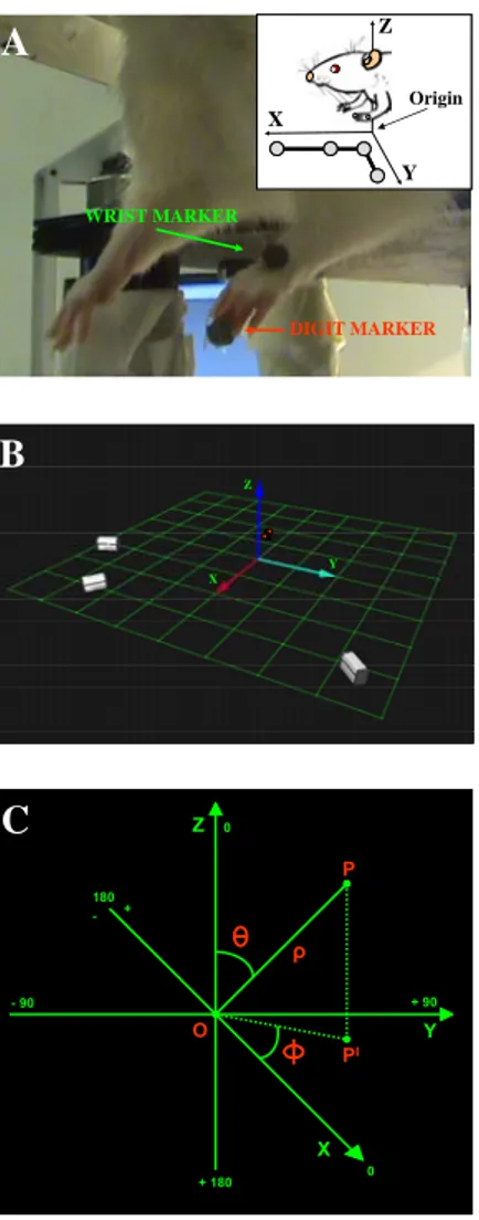
Movements evoked by long-duration ICMS were visually identified during mapping sessions and videotaped at 30 frames/sec by a standard camera. Evoked movements were examined and recorded with the animal supported in a fixed position in an elevated stereotaxic frame (Kopf). The body of the animal was laid on a table in a prone position with its forelimbs hanging down and free to move in all direction against gravity. The position of the trunk was stabilized to the back of the table to minimize spontaneous trunk movements (head/chest-fixed coordinates). The rest position for each forelimb was in approximately half-way extension-adduction and the wrist rested palm down, with the finger joints in semi extension (see Fig. 1A).

The recording video camera was positioned so as obtain a lateral or a frontal view of the animal. In order to detect the starting of the stimulus a triggered led was located near the body of the animal within the visual field of the camera. The video recording served as a back-up to clarify the data

analysis and gave information of the occurrence of the forelimb movements. Videotaped movements were analyzed frame-by-frame by using Quicktime and iMovie software.

2.3 Kinematic recording of complex movements and analysis

Movements evoked by long-duration ICMS were recorded and measured with a motion 3D optical analyzer (Qualisys Motion Capture System; Qualisys North America Inc., Charlotte, USA). 2 adhesive infrared-reflective spheres (diameter: 0.4-0.3 cm, weight: 0.04-0.05 g) were placed as a markers, on the forelimb skin over 2 anatomic landmarks: the wrist (head of the ulna), used to detect the limb movement and the last-phalangeal joint (tip) of the middle digit, used to detect the paw movement (Fig. 1A). The motion analysis system provided the 3D coordinates of the markers in space and it was then possible to reconstruct the ICMS-evoked movements. In order to minimize variability in marker positioning, markers in all experiments were placed by the same operator. 3 infrared cameras, placed around animals, were used to record position of markers (Fig. 1B). The cameras calibration has been conducted according to the Qualisys Motion Capture Analysis System proceedings. To do this, a stationary L-shaped reference structure with 4 markers attached to it placed under animals (see figure below and also Fig. 1A: box at the top right) defined the origin and orientation of the 3D coordinate system.

STATIONARY L-SHAPED REFERENCE STRUCTURE

STATIONARY L-SHAPED REFERENCE STRUCTURE

The direction of coordinate X-, Y- and Z-axis was anterior, lateral and vertical respectively. Movements were recorded for 2 seconds at a sampling rate of 100 Hz. Kinematic data will be analyzed off-line with Qualisys Track Manager software and with custom MATLAB programs to extract kinematic features. Recording trials were not considered for analysis when the fill level of recording was < 100%. This amounted to less than 15% of all trials. The start position of the forelimb was never modified during repetitive stimulations and recordings. Before each recording session, minor modifications of the forelimb positions were corrected to obtain the optimal visibility of the 2 markers within the calibrated field of the cameras. The purpose was to stimulate at the moment when the forelimb remained stationary in position of rest, so all stimulation trials took place in absence of spontaneous movement. In all animals, sham stimulation trials were recorded both while the animal was standing quietly with the forelimb stationary and while moving it spontaneously. The pattern obtained during sham stimulation was therefore unlike the pattern obtained during cortical stimulation at that site and unlike the pattern found at any stimulated site. Some spontaneous forelimb movement was observed at rest, however, in order to avoid interference between the evoked and spontaneous movement, a movement was detected as a displacement in XYZ-axes over a distance exceeding 5 mm. All measures was performed by subtracting the marker’s rest position in Cartesian coordinates from all points along the trajectory, thus all data sets began at (0,0,0). At first, the analysis was aimed to define the classes of movement and their topography across the cortical surface. Then, various kinematic parameters related to the limb and the paw component were determined from the analysis of the wrist and the digit marker separately and with different constrains. Moreover, the digit marker was evaluated in relation to the wrist marker.

Since a vertically component (Z-axis) was found in all evoked limb movements, the maximal displacement in one of the XY-axes defined the limb class of movement when it was over a distance exceeding 15% of the displacement in other axis. The displacement in Z-axis defined the type of movement when the displacement in XY-axes was < 5mm. We found that these values were

the most reliably to define the type of limb movement in all animals. When a displacement of both markers was observed the paw component of the movement was obtained by subtracting the wrist marker value to the digit marker value from all points throughout the movement. Thus, data sets of digit marker were defined by:

actual measures of digit markers values - actual measures of wrist marker values

In order to avoid interference between active and passive (transport limb depended) digit movement, a paw movement was detected as a displacement in 2 of the XYZ-axes over a distance exceeding 5 mm.

We computed the following kinematic parameters:  Maximal displacement in XYZ (MD:X,Y,Z);  Movement latency (L);

 Movement duration (D);

 Maximum peak velocity (MPV);  Mean velocity (MV);

 Number of peak velocity (PV);  Trajectory (T);

 Displacement vector (DV);  Path index (PI).

The start of movement (L) was defined by the frame at which the tangential velocity exceeded 5% of maximum velocity (Adamovich et al., 2001). The end of movement was defined by the last frame at which the marker reached the maximal displacement in one of the XYZ-axes. In this way the displacement toward the resting position and outlasting the stimulus was always outside the movement duration. All kinematic variables were calculated from the start to the end of movement (D). We determined the trajectory (T) and displacement vector (DV) from initial to final limb position for each stimulated site. Limb trajectory straightness was determined by the path index (PI)

index of 1 while the equal to a semicircle has an index of 1.57 (Archambault et al., 1999). In any case, a path index of greater than 1.57 represent either an S- or C- shaped or coil-like shape in sequences of movement. T and DV were used to determine the end-point 3D location of the limb, so they were considered only for the wrist marker. The number of peaks (PV) within the speed profile has been used to quantify the forelimb movement smoothness. Since the mean speed of movement was lower than its peaks, we count a pick when it was over the mean speed of the movement. In this study, peaks in speed represent decreases in smoothness or periods of acceleration and deceleration of movements evoked by a long-duration electrical stimulus. For each stimulated site the kinematic variables were obtained by averaging the values attained in 2-5 microstimulation trials.

2.4 Data presentation and statistical analysis

We used Multivariate Discriminant Analysis (MDA; Barker and McCombe, 1999) in order to analyse the displacement in XYZ-axes and kinematic variables for classifying movements in predefined classes. This method for analysing time-series biomechanical data allowed to determine the class of movement based on a set of variables known as predictors or input variables. The measure of confidence that the classification was correct and the measure of the predicted error rate on each classification were defined by:

 Proportion Correct = number of correctly classified samples/ total number of samples;  Error Rate = number of rejected samples/ total number of samples.

All individual displacements in XYZ-axes, were also plotted in 2D space (Fig. 3 and Fig. 8) to evaluate their spatial dispersions. To characterize the spatial distribution of all movements in the motor cortex across animals, a 2D distribution of movement-responsive sites at coordinate relative

to bregma was generated. Each movement-related site was taken to represent a square of 0.25 mm2

of cortical surface (0.5X0.5 mm) and 100% of probability in one site was achieved when a movement at that site was observed in all 7 animals (Fig. 4 and Fig. 9). We used the spherical

coordinate system (Fig. 1C) for physical 3D space evaluation of limb movement direction. Spherical coordinates is a coordinate system for 3D space where the position of a point is specified by 3 numbers:

 rho: is the distance of a point P from the origin. In present data rho was the limb movement vector length of value greater than 0;

 phi: was the angle between the X-axis and the ray between the projection of P onto the XY-plane and the origin; counter clockwise was considered the positive direction (phi: between 0 and ±180°);

 theta: was the angle between the Z-axis and the ray from the origin to P (theta: between 0 and 180°).

Multivariate test for difference in means (MANOVA) was used to compare displacement in XYZ-axes and kinematic variables. To analyze differences in kinematic means between classes of movement, one-way ANOVA followed by Tukey’s test were performed. Pearson correlation (r) significant at the 0.05 level was used to assess the relationship between kinematics variables. The reproducibility of kinematic measures between trials of repeated measures, was obtained calculated the coefficient of variation (CV = standard deviation/mean). All statistical procedures were performed in Minitab15 Statistical software features and in MATLAB (R2006a) applications for statistics and data analysis.

3. Results

Altogether, 339 sites were stimulated in the motor cortex of one hemisphere of 7 rats. The 41% of these sites was not considered for the result, since no markers displacement was evoked or the displacement in XYZ-axes was less than 5 mm (see Methods). Usually, these sites were located on the outskirts of the forelimb region delineating its border. In addition, forelimb movement were observed simultaneously with non-forelimb movements, as vibrissa, neck, hindlimb or mouth, near the borders between the forelimb area and these respective representations. In all animals, forelimb movements on the controlateral body side to the stimulated hemisphere were evoked. In addition some stimulated site evoked bilateral movements. At no site were forelimb movement evoked exclusively on the side ipsilateral to stimulating electrode. The mean stimulation threshold for evoking movements was 46.52 ± 2.36 µA. To facilitate the movement characterization, without altering its quality, all recordings were performed at 100 µA. The evoked movement proved to be repeatable from trial to trial and their features remained nearly constant over the time required to characterize each cortical site. Figure 2 shows a representative example of surface map of forelimb movements evoked by long-duration ICMS. In this scheme each of the forelimb site was characterized by movement of one or both markers. Overall, the limb movement (wrist marker) was evoked in 38.0% of sites, the paw movement (digit marker) was evoked in 11.5% of sites, and the limb-paw movement (both markers) was evoked in the remaining 50.5% of sites. A topography of complex movements was found, including the presence of 2 distinct forelimb areas (caudal and rostral forelimb area) in many cases not well separated from each other.

3.1 Stimulation-evoked limb (wrist marker) movements

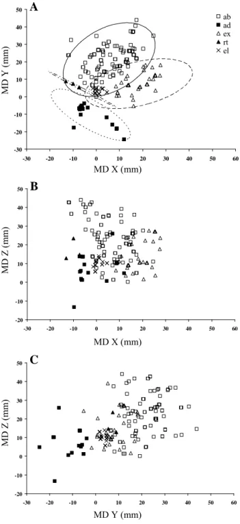
Long-duration ICMS elicited wrist marker movement in 177 out of 200 sites. Since a vertically component (Z-axis value > 5 mm, see Methods) was found in all evoked movements, we have classified movements according to the maximal displacement (MD) on the X or Y axis. According to MD (Tab.1), the repertoire of the limb movement included: abduction (ab, 55,37%, MD Y-axis positive), adduction (ad, 10,17%, MD Y-axis negative), extension (ex, 19,77%, MD X-axis positive), retraction (rt, 1.7%, MD X-axis negative) and elevation (el, 12.99%, Z-axis positive and X and Y axes < 5mm). The Multivariate Discriminant Analysis (MDA) classifier achieved an 88.1% correct classification rate with inputs of class of movement vs XYZ value. This indicates that 88.1% of the limb movements were assigned to the correct class (156 out of 177; P < 0.0001, MANOVA for XYZ vs Movement Class); 11.9% of false alarm rate was due to some ab (11 out of 98) and ex (6 out of 35) movements that the MDA classifier recognized as el movements. When all

individual displacements were plotted in 2D space, classes of movement were highlighted as a

cluster of points in the scatter plot of MD: X vs Y (Fig. 3A), conversely, the clusters of points were not well separated in the scatter plot of MD: X vs Z and MD: Y vs Z (Fig. 3B-C). Overall, these quantitative analysis suggested that movements were correctly classified. To characterize the spatial distribution of classes of movements in motor cortex across animals, a 2D frequency distribution bregma relative of limb-responsive sites was generated. Figure 4 showed a consistent topography in which cumulative sites were coded according to their rate. In this arrangement of stimulated effects, ab-related sites were clustered more posteriorly at coordinate corresponding the caudal forelimb region, ad-related sites were clustered more anteriorly at coordinate corresponding to the rostral forelimb region, ex-related sites were clustered at coordinate corresponding to the rostral forelimb region and the anterior part of the caudal forelimb region. The rt-related sites, was found to span the posterior border of the forelimb motor region. Unlike to other sites, el-related sites were scattered over the forelimb motor region so no overall topography was apparented. To evidence whether the topography of movements across cortical surface was associated with another

dimension of topography with respect to the limb direction, the sites were categorized according to their spatial end-points. The figure 5A showed an example of final end-points spatial map, derived from 1 animal. We have expressed the degree of spatial convergence in each stimulation site by calculating the coefficient of variation of the end-point coordinate. For each stimulation site, the coefficient of variation was expressed as the average of values from trial to trial (see Methods). The range of end-points variation in XYZ-axes among stimulated sites was 0.003-0.041, and the average coefficients of variation was 0.02 ± 0.019. This low values indicated that the stimulation in each site caused a significant spatial convergence of the limb toward a target location. To characterize the end-points spatial distribution across animals, we defined the vector movement spatial position in a 3D spherical coordinate system. In this system, each movement vector was made to origin from the intersection of axes while its length (rho) with the 2 angles (theta and phi), defined the final position of the wrist marker (Fig. 1C). Since el movements were carried out vertically upwards with negligible XY displacement, they were not considered for this computation. The MDA analysis confirmed the convergence for each class of movement toward a region of space in 3-Cartesian dimensions (Predictors: rho (mm)- theta- phi (grad) vs Movement class, N. correct: 137 out of 154, Proportion Correct = 0.89; P < 0.0001, MANOVA). This convergence can be seen in grater detail in the scatter plot of phi vs theta and phi vs rho (Fig. 5B-C), conversely there was no clear spatial clustering between the class of movements in the plot of theta vs rho (Fig. 5D). These results showed that similar spatial map of end-points was a consistent feature of the limb motor cortex in all mapped animals, and suggested that the spatial map of the limb movement was strongly related to the azimuthal (latitude) component of the movement in the 3-Cartesian dimension.

3.2 Limb (wrist marker) movements kinematics

Table 2 sums up the kinematic variables calculated from the wrist marker during the limb

movement. A significant interaction was observed for movement latency and duration (L: F(4,175) =

5.06, P = 0.001; D: F(4,176) = 3.78, P = 0.006) between the class of movements. As shown by

post-hoc analysis, ab movement had a significant shorter latency (T = 4.16, P = 0.0005) and longer duration (T = -2.98, P = 0.026) when compared to ad movement. With regard to the velocity variables, no significant effect of class was found for maximum velocity, conversely, a significant

interaction was found between class for mean velocity (MV: F(4,172) = 2.66, P = 0.035) and peak

velocity number (PV: (F(4,176) = 11.74, P < 0.0001). It was found that the ex movement showed a

significant higher MV (T = 3.85, P = 0.026) compared to el movement and a significant higher PV compared to ab (T = 6.34, P < 0.0001), ad (T = 5.3, P < 0.0001) and el movement (T = 3.85, P = 0.002) while ab, ad and el movements did not significantly differ from each other in these respect. There was found to be a highly significant main effect of class on trajectory length (T: F(4,176) =

13.10, P < 0.0001) and vector length (DV: F(4,176) = 26.72, P < 0.0001). The post-hoc test revealed

that the class differences found by means of T and DV, were mainly related to the fact that ab and ex movement had significantly greater value in both T and DV in comparison to other class of movements (all comparisons: P < 0.0001). Furthermore the post-hoc comparison revealed that ab movement significantly different from ex movement in virtue of shorter T (T = 3.34, P < 0.009) and longer DV (T = -3.96, P < 0.002). We tried to estimate whether the trajectory lengths were consistent trial by trial in each stimulated site. On repeated trials with the same stimulation parameters, the average coefficient of variation (SD/mean) of T was 0.17 ± 0.1 (range: 0.01-0.32). Then we have evaluated the ICMS-evoked T degree of straightness, using the path index (PI: see Methods). All trajectories had a curved shape (PI > 1) and only the 32.9% had a PI below 1.57. The trajectories with a PI > 1.57 exhibited a general C- or S-like shape, while only the 6% had a coil-like shape (Fig. 6). Notably, coil-coil-like trajectory were found only in the 25.7% of ex movements. In agreement with this finding, the ex movement showed a PI number of 3.72, significantly and

considerably greater that other movement PI (F(4,176) = 9.89, P < 0.0001). The correlation analysis

was used to describe the relationship between multiple kinematic variables presented in the Table 2. Correlations were positive between D and T (r = 0.18, P = 0.01) and DV (r = 0.265, P < 0.0001) conversely, correlations were negative between L and D (r = -0.23, P = 0.002) and DV (r = -0.41, P < 0.0001). There was a strong positive correlation between T and kinematic variables of velocity (MV: r = 0.4, P < 0.0001; MPV: r = 0.57, P < 0.0001) and the PV (r = 0.58, P < 0.0001).

3.3 Stimulation-evoked paw (digit marker) movements

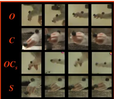
It was observed ICMS-evoked digit marker movement in 124 sites out of 200 sites. As can be seen from the video sequences (Fig. 7) and MD values (Tab. 3), paw movements included: opening (O: 66.1%, MD X positive), closure (C: 5.6%, MD X negative), opening/closure sequence (OCs: 9.7%, opening phase MD X positive, followed by closing phase, MD X negative) and supination (S: 18,5% MD Z positive). We asked whether opening and closing phase in OCs were different from O and C movement, respectively. The MDA classifier achieved an 73.9% correct classification rate with inputs of class of movement vs XYZ value (N. correct: 137 out of 154; P < 0.0001, MANOVA). The false alarm rate (26.1%) was largely due to the low discrimination between O and

the OCS opening phase (O Proportion Correct: 0.67; opening phase of OCs Proportion Correct:

0.58). Conversely, MDA classifier achieved a 100% classification rate for C and the OCs closing phase. All these aspects of paw movements, can be seen in greater detail when all individual displacements were plotted in 2D space. As showed in the Fig. 8, the clusters of points were not

well separated in the MD plot of X vs Y (Fig. 8A), conversely, classes of movement were clearly

clustered in MD plot of X vs Z (Fig. 8B). Notably, the overlap of O and OCs opening phase points in all 3 plots. O, C, and OCs movements characterized by simultaneously digits contraction; S movement characterized by wrist external rotation without fingers movement. Moreover, O, C, and S movements appeared as a single movement in each single trial, conversely, the OCs movement characterized by repetitive sequences of opening and closing phase in each single trial (mean of

sequences: 5.03 ± 0.5, range 4-8). Thus, these analysis together suggested that O, C, OCs and S were different classes of paw movement. The bregma relative frequency distribution of paw-responsive sites showed a consistent topography of class of movement across the cortical surface (Fig. 9). The O movement was elicited in a portion of the forelimb region, where the stimulation most often elicited ab movement while the C and OCs movement was elicited in a portion where the stimulation most often elicited ad or ex movement. Finally, the S movement was elicited in a more lateral portion of the forelimb region where limb movement was less commonly elicited by electrical stimulation.

3.4 Paw (digit marker) movement kinematics

Table 4 sums up the kinematic variables calculated from the wrist marker during the paw movement. The MDA classifier achieved a high level of classification rate with input of kinematic variables vs class of movement (Predictors: Kinematic variables vs Movement Class, N. correct: 98 out of 124, Proportion Correct = 0.79; P < 0.0001, MANOVA). All paw movements began at short latency after the stimulation (L mean: 27.47 ms) and no significant difference in L between the

classes of movement has been detected (F(3,123) = 0.92, P = 0.43). There was no significant

difference in D between O, C and S movements (all comparisons T > 0.5, P > 0.7); conversely, the OCs movement had longer D in comparison to other classes of movement (all comparisons T > 4.9, P < 0.0001). With regard to the MV, the C movement proved faster than the O movement (MV: T = 3.01, P = 0.017). In OCs movement the PV was significantly higher than the other classes of movement (all comparisons: T > 12.1, P < 0.0001) that did not significantly differ from each other in this respect (all comparisons: T < 0.1, P > 0.9). Notably, in OCs movement, PV were at the opening phase of the movement. Finally, S movement proved much slower than movements involving the fingers (all comparisons, MPV: T > 3.5, P < 0.004, MV: T > 4.17, P < 0.0001).

3.5 Relation between limb and paw movement

Limb-paw movements accounted for half of all stimulation-induced forelimb movement (101 out of 200 sites). There was no clear topography of sites that showed limb-paw movement and sites that did not; both types of sites were intermingled in cortex. A specific pattern of limb and paw movement combination existed. Specifically, O movement was combined with the ab movement (63.4%), ex movement (18.3%) or el movement (18.3%). With regard to the placement of the maximum paw opening as a percent of the total limb movement, it was found that the paw maximum opening occurred at 73.0% of ab movement and at 100.3% and 95.7% of ex and el movement, respectively. Note that, the O movement duration did not change when it was combined

to ab, ex or el movement (F(2,81) = 0.51, P = 0.601). The C movement was always combined with ad

movement and its maximum closure occurred at 191.0% of ad movement. The 28.64% of ad-C movements involved a time-synchronized mouth opening. The OCs movement was always combined with ex movement and sequences occurred over 135.69% of the time needed for the ex movement. There was also found that in the ab-O movement, the ab had a significant shorter latency in comparison to O (ab vs O: 24.04 vs 29.62 ms; F(1,103 )= 7.75, P = 0.006). In other

limb-paw movement combinations the latency value was equal in both the limb and limb-paw component then, in these movements the motions at the involved joints began almost simultaneously.

4. Discussion

In the discussion of this doctoral thesis, we have the goal of showing how the long-duration ICMS has the potential to reveal a better characterization of the organization of the forelimb motor cortex in the mammals and specifically, how it is useful for understanding the strategy governing the organization of the forelimb map in rat’s motor cortex.

Our findings have shown that long-duration stimulation paradigms result in reproducible activation of groups of forelimb muscles to achieve complex movements which may be set out in terms of their kinematic properties. The electrically-evoked movements were described in terms of 3D displacement and kinematics variables recorded from 2 markers positioned on the wrist and middle digits of rat’s forelimb. The results confirmed and extended previous findings that have documented the existence of complex movement representations within the motor cortex of monkeys (Graziano et al., 2002; Gharbawie et al., 2011; Stepniewska et al., 2011) and rats (Ramanathan et al., 2006). The quantitative analysis of markers separately allowed to define 5 classes of limb movements (ab, ad, ex, rt, el) and 4 classes of paw movements (O, C, OCs, S). In half of all forelimb-related stimulated sites a specific pattern of limb and paw movement combination existed. The present finding provide insight regarding internal organization and distribution of patterns of complex movement in the rat’s forelimb motor cortex.

4.1 Methodological and Technical remarks

In this study, the long-duration ICMS was combined with the motion 3D analysis of the ICMS-evoked forelimb movement. To our knowledge, this is the first study to use the motion analysis to asses the reproducibility of kinematic measures of ICMS-evoked complex forelimb movement in rats. The idea of combining these techniques might be well suited when motor cortical output is intended to be quantified and components of ICMS-evoked movement (limb and paw movement) have to be objectively assessed and documented. Because the markers were attached at the wrist

and middle digits, it was predicted that the limb and paw movement had a large prevailing effect on wrist and digit marker, respectively. This allows the investigation of whether the subcomponents of complex movement follows a gradient into the rat’s forelimb motor cortex. To this end, a 3D recording system generally used to record kinematics in humans and monkeys has been adapted to recording kinematics in rats. The system our group used for kinematic assessment of forelimb movements was an infrared-based motion analyzer. Alternative systems used ultrasound, electromagnetic or video-based signals to investigate the spatio-temporal characteristics of forelimb movement. All systems appear to have comparable sensitivity and reliability. An advantage of infrared reflecting markers was that this system work wireless and is easily interfaced with a video camera and with data processing systems. Moreover, this system has proved suitable to record kinematics with small neighbours markers on a small forelimb. Rats were suitably positioned on the stereotactic system within the calibrated space to obtain stable and reproducible kinematic measures on repeated recordings and to establish a range of values for reliability of kinematic measures. Here we used conditions in which the full expression of neural, muscular, and biomechanical occurred. The evoked forelimb movements were made against gravity, as would natural movement, although the forelimbs hanging position with the head fixed to the stereotactic under anaesthesia was not a natural setting.

Asanuma and Arnold (1975) found that trains of cathodal pulses killed the cortical tissue around the electrode tip. With balanced biphasic pulses it is possible to stimulate for long durations and high current without measurable damage (Theovnik, 1996). Our stimulation paramenters are within the range of cortical stimulation studies in oculomotor, visual, and sensory-motor system (Bruce et al., 1985; Freedman et al., 1996; Gottlieb et al., 1993; Romo et al., 1998; Salzman et al., 1990; Tehovnik and Lee, 1993). Finally, in present experiments using the same stimulation techniques in rat, on histology no visible damage to the cortex associated with the stimulation was found.

How much did the effects of ketamine anaesthesia contribute to the patterns of evoked movement observed in the present study?

Ketamine takes effect by selective blockade of NMDA receptors leaving fast transmission by AMPA and, notably, GABA receptors intact (Ebert et al., 1997; Sonner et al., 2003). In contrast to other anaesthetics, the spontaneous firing rate and sensory evoked cortical activity are enhanced (Kayama et al., 1972) and a comparable pattern of cortical excitation and inhibition after ICMS was observed in ketamine-anaesthetized and awake animals (Butovas and Schwarz, 2003). Moreover, in the ketamine-anaesthetized animals, stretch reflexes, flexion reflexes, and reciprocal inhibition between antagonistic muscles are manifest (Capaday et al., 1998; Schneider et al., 2001). Thus, in the present experimental condition, we characterized how activation of corticospinal inputs to the spinal cord activated from separated sites of motor cortex produced patterns of motor output. Supports for this notion comes from the finding of very similar motor patterns of vibrissae movement in ketamine-anaesthetized rat and in absence of general anaesthesia (Haiss and Swarz, 2005).

The complex movements elicited by the long trains of electrical pulses likely activate complex circuits locally about on the electrode tip and in projection sites that includes neurons in a number of cortical and subcortical structures. The manner in which extracellular current activate complexly organized neural tissues is only partly understood. Basically, 3 interdependen aspects have to be considered to understand the effect electrical stimulation have within the nervous tissue. First, the exact extent and shape of the directly activated brain area has to be known. There is a vast literature on the neural elements activated by electrical microstimulation (e.g., Ranck, 1975; Doty and Bartlett, 1981; Yeomans, 1990; Tehovnik, 1996; Rattay, 1999). Despite this, we still know very little about the local and distal brain circuits recruited during the delivery of currents to brain tissue. It is a generally accepted simple rule that electrical microstimulation leads to a sphere of activated neurons around the electrode tip that increases in size with the increasing current so that larger currents activate neurons at a larger distance from the electrode (Stoney et al., 1968; Theovnik et al., 1996; Tolias et al., 2005). In early ICMS studies a single stimulation protocol with single-cell recording was used to deduce the current spread and the direct excitability of pyramidal neurons

within motor cortex of cat (Asanuma et al., 1976; Stoney et al., 1968). It has been estimated that 200 µs pulses with 10 and 100 µA amplitude activate cells in a radius of 100 and 450 µm around the electrode (Stoney et al., 1968). The second problem to be considered is which different neuronal part like dendrites, somata, and axons to be directly activated. The direct excitability (chronaxie) of cortical neurons expressed as the pulse duration at twice of rheobase current was found ranging between 0.1 and 0.4 ms (Asanuma et al., 1976; Stoney et al., 1968). Axons have shorter chronaxies than those of cells bodies and large myelinated axons have shorter chronaxies than those of small, non-myelinated axons (Ranck, 1975). According to these experiments, it is accepted that using 0.2 ms pulses of current the sites of direct activation of cortical neurons are the initial segment and nodes of Ranviers of large myelinated axons (Jankowska et al., 1975; Nowak and Bullier 1998, I,II; Rattay, 1999). Some investigators have used behavioural methods to estimate the spread of electrical stimulation within neocortex (Murasugi et al., 1993; Tehovnik et al., 2004 and 2005). Theovnik et al. (2004) found that the amount of V1 tissue activated with 50-100 µA current (with 100 ms trains using 0.2 ms pulse delivered at 200 Hz), was estimated to be 0.572 and 0.736 mm, respectively, from the electrode tip and the chronaxie of exited elements ranged between 0.1 and 0.4 ms. Recently, fMRI (functional Magnetic Resonance Imaging) that relies on the BOLD (Blood Oxygen Level-Dependent) signal was used to study the spread properties of electrical stimuli delivered to V1 cortex in anesthetized monkey (Tolias et al., 2005). These experiments found that for current levels of 159 to 1,651 (4 sec train duration of 0.2 ms pulses at 100 Hz) the amount of activated tissue ranged from 2 to 4.5 mm from the electrode tip. This extensive spread of current as measured with fMRI is consistent with the spread observed using optical imaging of neocortex where lower currents were used (Seidemann et al., 2002). In other word, electrophysiological, behavioural and imaging methods produced very similar chronaxie values that fell between 0.1 and 0.4 ms, by contrast, they produced different current spread estimates for cortical stimulation. Specifically, electrophysiological and behavioural methods yielded estimates of activity spread that were comparable and imaging methods yielded estimates roughly fourfold greater than those

observed using other methods (for review see Theovnik et al., 2006). A main reason that could account for the observed difference between imaging data and other measures of current spread might be related to transynaptic activity that imaging techniques are able to direct visualize. This insight represents the third problem to be solved: the direct activation of the somata is mated with axonal excitation carrying the activation by ortho-antidromic conveyance of spikes on interconnected structure (indirect effects). Because axons are abundant in neocortex, local antidromic and synaptic effects must be expected to carry the major part of the stimulation effect, especially using long-duration protocol of stimulation. Indeed, it is well established that even single electrical pulse delivered to cortical tissue is able to activate trasynaptically cortical neurons beyond the site of direct stimulation (Asanuma and Rosen, 1973; Jankowska et al., 1975; Butovas and Schwarz, 2003). The transynaptic activation as measured with imaging techniques may be dominated by subthreshold responses (Mathiesen et al., 1998; Logothetis et al., 2001) or might also indicate the presence of spiking activity. The lateral spread of the fMRI response beyond of the local direct stimulation might be related to the activation of local horizontal connections and cortico-cortica and/or sub-corticall projections. Recently, results suggest that electrical stimulation of cortex elicited positive BOLD responses in topographically matched regions of cortex all of which are monosynaptic targets of the stimulated site (Tolias et al., 2005) and evidenced for the lack of electrically induced polysynaptic propagation of activity in the neocortex (Sultan et al., 2011). Despite this large number of investigation on ICMS, there is only coarse information about the location of the activated cortical neurons and their distribution at a distance from the stimulating electrode tip. Recent data on cortical excitation with microelectrode has shed new insight on mechanisms involved in ICMS evoked movements. From past studies, using optical technique imaging (Smetter et al., 1999; Stosiek et al., 2003), it know that somatic calcium in cortical neurons largely reflects action potential firing, rather than sub-threshold events. In vivo cortical networks experiments, the 2-photon imaging technique allows for direct imaging of hundreds of activated cortical neurons around the electrode tip (Sato et al., 2007; Kerr and Denk, 2008). Using this

technique it was found that intracortical microstimulation directly activates a sparse, distributed population of neurons around the electrode even at low currents (Histed et al., 2009). The stimulation protocols used by Histed and coll. matched protocols used in previous studies of the influence of cortical circuits on behaviour and also partially matched the protocol of stimulation used in our experiments. They used constant-current biphasic square pulses, each phase lasting 200 μs, with the negative pulse first (Theovnik, 1996) at 250 Hz in trains of 100 to 814 ms at low (≤ 10 μA) currents. The cortical stimulation near threshold produces a sparse and distributed set of activated cells in a way that a small fraction of all neurons were activated. Some of activated neurons were located hundreds of microns away from the electrode tip, while other nearby cells did not respond (Histed et al., 2009). Well known electrophysiological data support the idea that axons near the electrode tip are the main neural elements activated by threshold current stimulation (Theovnik et al., 2006). Histead and coll. suggest that the sparse patterns of activated cell observed at threshold were largely independent of synaptic transmission. According with this conclusion, the pattern of activated cells depend strongly on electrode position in a way that moving the electrode tip 30 μm almost completely eliminated overlap of activated neurons. Activating processes near the tip gives a ball of activated cells, but even near threshold this ball is sparse. Larger currents recruit more neurons, producing greater postsynaptic summation to result in postsynaptic spiking (Stoney et al., 1968; Butovas and Schwarz, 2003) so that increasing current instead of activating cells at greater distance causes the ball to fill in as more cells are activated.

The neocortex contains several excitatory and inhibitory neurons that are complexly interconnected locally as well as over large distances (Braitemberg and Schüz, 1998). This high interconnectivity of the neocortex suggest that a close correlation of both excitatory and inhibitory effects were induced after electrical stimulation. The common finding was that a postsynaptic sequence of fast excitation and long-lasting inhibition response of neocortex has been demonstrated after intracortical microstimulation (Asanuma and Rosén, 1973; Shao and Burkhalter, 1996; Chung and Ferster, 1998; Butovas and Schwarz, 2003; Logothetis et al., 2010). Recentely the effects of

microstimulation on cortical elements was better understood using a multielectrode recordings (Butovas and Schwarz, 2003). Assessing spatial electrical parameters of the stimulation indicated that stimulation frequencies at > 20 Hz evoked repetitive excitatory responses standing out against a continuous background of inhibition. The inhibitory response that follows the fast excitatory response was remarkably static in its temporal characteristics indeed, it is unaffected by stimulus parameters and its takes > 100 ms beyond the duration of the stimulus (Butovas and Schwartz, 2003). These features suggested that it is the activation of synaptic inhibition mediated by GABAb receptor that plays a major role in generating prolonged inhibition after stimulation (Butovas et al., 2006). All these new technical studies are useful to recast the interpretation of studies that used microstimulation to affect cortical activity, and can address the interpretation of our results.

4.2 Why long-duration ICMS of the forelimb motor cortex evoked patterns of coordinated movement

Stimulation of the cortex is non-physiological, and thus the results should be taken cautiously. However, ICMS experiments exposed above can be helpful in explaining why long-duration ICMS of the forelimb motor cortex evoked coordinated movement responses. Moreover, it is important to consider whether the complex movement elicited by long-duration ICMS reflect the activation of motor networks associated with behavioral relevant movements. Typically, in the present experiments at each cortical site, the stimulating current was increased gradually until a clear multijoint movement of the forelimb was detected (current threshold for movement, see Methods). Thus, our explanation for this is that threshold currents recruit neurons, producing postsynaptic summation (Stoney et al., 1968; Butovas and Schwarz, 2003) that resulted in a multijoint forelimb movement evoked 50% of the time. Increasing current to about twice threshold (100 μA), instead of activating cells at greater distance, probably caused the activation of more cells around electrode tip (Histed et al., 2009) and so, a clear, consistent, multijoint movement of the limb was obtained for recording. In rat motor cortex horizontal projections extending laterally by 0.5 to 1 mm could

concur to the lateral spread of electrical response beyond the fringe of direct stimulation. Thus, we can suppose that in our experiments the mechanism of activation was local with a focus on transynaptic effects so that moving the electrode by 500 μm changed the pattern of activate neurons (Histed et al., 2009). It is possible that the ICMS-evoked complex movement may be caused by the activity of a neuronal population significantly larger than neurons activated directly as a result of the passive spread of current. Yet it is possible that ICMS as used in the present experiments activates directly the most excitable elements of the motor cortex and that these elements tend to project to other cortical areas as well as subcortical networks, connected monosynaptically to the direct excited neurons (Logothetis et al., 2010) and involved in the generation of the forelimb movements. Some authors (Strick, 2002) have argued that the long-duration ICMS may lead to nonspecific current spread, generating complex movements by randomly activating a large number of spinal motorneurons. According to this interpretation, the nonspecific and randomly activated spinal motor neuron would result in massive, stereotyped movements, most similar to massive contractions during local or general seizures than to those of voluntary action. Alternatively, if the random activation of multiple simple movements contributing to a complex sequence one would expect that the order of movement in sequences also would be random based on the pseudorandom activation of neurons within the motor cortex. Moreover, long stimulus patterns at high frequencies, as used in the present study, have been shown to elicit a strong and continuous inhibition in neurones residing within a large area surrounding the electrode that could limit the current spread from the stimulation site (Chung and Ferster, 1998; Butovas and Schwarz, 2003). In all our experiments, the long-duration ICMS evoked sequential activation of groups of muscles that shape reproducible patterns of forelimb movements. As in other similar results (Graziano et al., 2002; Ramanathan et al., 2006; Gharbawie et al., 2011), several aspect of our results, suggest that the stimulation-evoked movements may mimic normal one, indeed, in all recorded cases, the movement appeared to be natural and coordinated and we never evoked twisted or unnatural patterns of movement. Thus, we can conclude that the movement appeared to be natural because long-duration

ICMS probably recruits neurons in many parts of the motor-sensory networks and this recruitment of neurons presumably occurs every time we make a natural movement at the same time scale. One of more interesting result of this study, indicates that in the 50% of stimulated sites, ICMS evoked coordinated forelimb movements involving proximal (shoulder and elbow) and distal (wrist and digit) segments. These sites were dispersed over the forelimb motor region, that is in the proximal as well as in distal forelimb motor area. In rats, the C8 spinal cord segment contains lower motor neurons that activate muscles controlling distal forelimb movements required for grasping, whereas motor neuron pools located in the C4 spinal segment are associated with control of proximal forelimb, shoulder and neck musculature (McKenna et al., 2000). There was abundant evidence that neurons related to distal and proximal actions intermingle considerably within M1 in both primate (Donoghue et al., 1992; McKiernan et al., 1998; Park et al., 2001) and rat (Wang et al., 2011) and that neuron population in a small region of M1 can encode information related to kinematic variables of naturalistic movement of the upper limb (Vargas-Irwin et al., 2010). Within the rat’s motor cortex, both C8- and C4-projecting neurons are anatomically distributed throughout the forelimb region, describing an interspersed network of motor neurons that do not collateralize across the C4 and C8 spinal segments (Wang et al., 2011). Our results support the notion that distal forelimb-projecting and proximal forelimb-projecting neurons are intermingled within motor cortex, and could suggest that corticospinal motor neurons were segregated on the basis of their contribution to specific aspect of motor control during naturalistic movements. In rats descending pathways from motor cortex terminate largely on interneurons in the intermediate zone of the spinal cord and lack substantial direct input to motoneurons (Catsman-Berrevoets and Kuypers, 1981). Indeed, it is a common point of view, that the rat’s cortico-spinal system utilizes the integrative mechanisms of the spinal cord to generate a range of skilled motor behaviour. Our observations suggest that the activation of proximal and distal segments in ICMS-evoked complex forelimb movement may occur directly within the activated motor cortex. This interpretation do not exclude

that subcortical networks (cerebellum, basal ganglia, and spinal circuits) could be involved in the sequential activation of groups of muscles in electrically evoked forelimb movements.

5. Figures

Tab. 1 Wrist marker maximum displacement (MD)

Class MD X(mm) MD Y(mm) MD Z(mm) abn=98 5.53 ± 0.83 21.72 ± 0.82 22.99 ± 1.14 adn=18 -2.40 ± 1.65 -10.29 ± 1.42 7.61 ± 1.95 exn=35 19.33 ± 1.45 7.92 ± 0.96 14.61 ± 1.50 rtn=3 -10.13 ± 1.67 7.26 ± 0.98 17.01 ± 3.28 eln=23 0.76 ± 0.34 3.08 ± 0.26 10.17 ± 0.50

Tab. 1: Mean scores (± SEM) of maximum displacement (MD) in XYZ-axes measured (mm) of the

wrist marker classes of movement: ab, abduction; ad, adduction; ex, extension; rt, retraction; el, elevation; n: number of sites for each class.

Tab. 2 Wrist marker kinematics

Class L(ms) D(ms) MPV(mm/s) MV(mm/s) PV(n) T(mm) DV(mm) abn=98 23.46 ± 0.69 506.80 ± 15.20 428.00 ± 18.60 128.70 ± 13.60 2.32 ± 0.08 60.82 ± 3.04 29.15 ± 0.97 adn=18 31.11 ± 2.12 387.20 ± 45.20 476.9 0 ± 41.40 98.60 ± 11.10 1.94 ± 0.22 32.77 ± 2.57 13.91 ± 1.44 exn=35 26.18 ± 1.20 434.90 ± 23.30 492.20 ± 32.10 157.60 ± 12.60 3.97 ± 0.33 82.88 ± 9.23 22.26 ± 1.71 rtn=3 23.33 ± 3.33 473.00 ± 107.00 273.6 0 ± 720 77.10 ± 15.70 2.00 ± 0.00 35.50 ± 1.61 20.57 ± 3.23 eln=23 26.96 ± 1.47 414.30 ± 36.40 376.40 ± 42.40 70.89 ± 8.85 2.60 ± 0.39 26.05 ± 1.88 11.21 ± 0.54

Tab. 2: Mean scores (± SEM) of kinematic variables of the wrist classes of movement (see caption

in Tab. 1). Kinematic variables were: L, movement latency; D, movement duration; MPV, maximum peak velocity; MV, mean velocity; PV, number of peaks velocity; T, trajectory; DV, displacement vector. Units: ms: milliseconds; s: seconds; mm: millimetres; n: numbers.