SISTEM: a new method to integrate geodetic and satellite data to estimate 3D ground deformation maps

Università degli Studi di Catania

FACOLTÀ DI INGEGNERIA

DIPARTIMENTO DI INGEGNERIA ELETTRICA ELETTRONICA E DEI SISTEMI

TESI DI DOTTORATO DI RICERCA IN INGEGNERIA ELETTRONICA, AUTOMATICA E CONTROLLO DI SISTEMI COMPLESSI

XXIII CICLO

A

LESSANDRO

S

PATA

SISTEM: a new method to integrate geodetic and satellite data to

estimate 3D ground deformation maps

Coordinator:

Prof. L. Fortuna

Tutor: Prof. G. Nunnari

Acknowledgements

A sincere thank goes to my tutor Prof. Giuseppe Nunnari who, first, gave me the chance to spread my wings toward research and who always represents for me a sample of scientific rigor and devotion.

I would like to express my gratitude to Dr. Giuseppe Puglisi for giving me the opportunity to work in the interesting area of Volcano Geophysics and for his guidance, support, and advice throughout these studies.

I am indebted to “Istituto Nazionale di Geofisica e Vulcanologia” for providing the financial support throughout the Ph.D.

I am grateful to the members of the research groups of the “Unità Funzionale Deformazioni del Suolo” at INGV for their support; especially to Dr. Francesco Guglielmino and Dr. Alessandro Bonforte for their useful assistance. I am grateful to other members of the INGV of Catania, Eng. Michele Prestifilippo, Eng. Gaetano Spata, Eng. Flavio Cannavò, Eng. Dino Montalto. Whenever I had problems in my research they was always there to help me.

I would like to thank my family, my parents, and my brothers to be always ready to encourage me.

Index

Introduction ……… 5

Chapter 1 State of the art ……… 9

The S. Gudmundsson and F. Sigmundsson method ………. 9

Problem formulation ……….. 9

An introduction to the Markov Random Field Regularization and Simulated Annealing ……… 11

Construction Process ……… 13

Energy Functions ……… 15

Simulated Annealing Optimization ………. 18

Parameters ……….. 20

The Samsonov and Tiampo method ……… 23

Theoretical background ……….. 23

GPS and DInSAR analytical integration ……… 26

Chapter 2 The SISTEM method ……… 30

Introduction ……… 30

Mathematical Background ……… 31

The Simultaneous and Integrated Strain Tensor Estimation from geodetic and satellite deformation Measurements (SISTEM) approach ………. 34

A Synthetic case study ……… 36

A real case study performed on the Mt Etna area ……… 45

Chapter 3 Modeling ……….……….. 54

Introduction ……… 54

An Inverse Modeling method based on Particle Swarm Optimization ……… 54

Chapter 4 Toward a more realistic volcanic source shape ……… 63

Introduction ……….. 63

Artificial Neural Network background ………. 64

Methodology ……… 67

Case study ……… 71

Conclusions ……… 74

Appendix ………. 78

A new method based on the Lagrange multipliers to reduce phase error affecting DInSAR data ……….. 78

Introduction

The aim of this work is to propose a new method in order to efficiently produce high-resolution maps relevant to the three-dimensional motion of Earth’s surface by combining information from sparse Global Position System (GPS) measurements and Differential Interferometric Synthetic Aperture Radar (DInSAR) data.

The use of DInSAR and GPS data to monitor ground deformations on the same active tectonic or volcanic areas are extensively used [1]; Plate Boundary Observatory (PBO) web-pages at UNAVCO http://pboweb.unavco.org/].

Nevertheless, each technique has some significant shortcomings when used in a stand-alone mode. Although GPS is the most suitable technique for measuring ground deformation with sub-cm accuracy level, it provides a point wise 3D displacement vector referring to the specific geodetic benchmark where the antenna is set up; consequently, the spatial resolution of the measurement of the ground deformations depends on the network geometry and thus is usually low (in the order of a few points / km2, in the optimal conditions). DInSAR provides displacement measured along the Line Of Sight (LOS) between the Earth’s surface and the sensor; for satellite systems, which have off-nadir angles of about 20°-40 °, this implies that DInSAR measurements are more sensitive to the vertical component of the deformation than to the horizontal ones. Since the DInSAR measures along a specific direction (LOS), the dimension of the information on the ground deformation is a scalar. The DInSAR surveys provide maps of the Earth’s movements having pixel size in the order of 20 m × 20 m; thus the spatial resolution is higher than the GPS network. The accuracy of the DInSAR measurements is in the order of the cm, being the knowledge of the orbits, the accuracy of the

first two, which can be reduced by adopting specific procedures, the atmosphere (and in particular the troposphere) is at the origin of the main unpredictable perturbing effects. The variations of the troposphere may affect the ground deformation measurements over ten of centimetres in very unfavourable conditions due, for instance, to turbulences on mountainous areas [2]. However, the atmospheric signal follows, on the whole, the power law distribution and in general we may expect effects in the order of 0.5-1 interferometric fringe (e.g. ~ 1.5-3 cm, for a C-band SAR [3,4] [Bonforte et al., 2001, Mattia et al., 2007]. Several techniques have been proposed during the last decade to reduce or eliminate the tropospheric effects on DInSAR data [5, 6, 7], but none of these can be considered as definitive and each of these has pro or cons depending on the specific experimental conditions. .

The integration of DInSAR (scalar) data with the GPS (vector) data should provide information on the ground deformations by taking advantage of the positive features of both these techniques, i.e. the high spatial resolution of the DInSAR, the 3D measurements and the sub-cm accuracy level of GPS. This integrated information should be able to give a more reliable interpretation of the geophysical phenomena producing ground deformations.

Recently, a few methods aimed at integrating these two kinds of data have been published [8, 9]. Gudmundsonn et al. [8] applied a Bayesian statistical approach and Markov Random Field (MRF) theory to derive 3-D velocity maps, while Samsonov and Tiampo [9] introduced an analytical optimization of interferometric observation and GPS dataset. Apart from the differences in the algorithms used for combining the data, these two methods have two points in common: the first is the preliminary interpolation step in which sparse GPS measurements are interpolated in order to fill in GPS displacements at the DInSAR grid and the second one is that the optimization techniques used to combine the different datasets are not based on the physics of the deformations (i.e. from the elasticity theory).

The interpolation technique typically used in these two methods is the kriging which requires for each component to be interpolated, the choice of an appropriate theoretical semivariogram model. This choice is one of the main critical points in geostatistics [10] and it is usually performed by supervising a preliminary statistic analysis of the experimental data.

Here we propose the SISTEM (Simultaneous and Integrated Strain Tensor Estimation from geodetic and satellite Measurements) method, a Weighted Least Square (WLS) approach totally based on the elastic theory, to simultaneously integrate GPS and DInSAR data without requiring the preliminary step of the GPS interpolation. In this way, the dependence on the choice of the theoretical semivariogram model, required by the kriging interpolator, is avoided. Furthermore, this method computes the results on each point of the Earth’s surface and, being based on elastic theory, it provides the 3D strain and the rigid body rotation tensors. The estimated standard errors computed by the WLS for each computation point are also provided to assess the reliability of the results.

Furthermore 3D ground deformation maps, obtained thought the SISTEM method, were used in the framework of the inversion problem. In this context an inversion procedure based on the joined use of a Particle Swarm Algorithm and the Gauss-Newton optimization methods was used to solve the inversion problem relevant to the 2009 Abruzzo earthquake. Moreover, other novelty of this work, a neural network based approach aimed to estimate more realistic volcanic source shape instead of perfect geometric source shape was proposed.

This work is organized as follows. In chapter 1 the state of the art relevant to the integration of geodetic and satellite data to obtain 3D motion maps over the whole investigated area is reported. In particular the methods developed by S. Gudmundsson and F. Sigmundsson [8], Three-dimensional surface motion maps estimated from combined interferometric synthetic aperture radar and GPS data, and the method developed by Samsonov and Tiampo [9],

Analytical optimization of InSAR and GPS dataset for derivation of three-dimensional surface motion, are reported. Chapter 2 describes the new method we have developed in order to integrate geodetic and satellite data. Chapter 3 is devoted to the inversion modeling problem. In chapter 4 a new method based on Artificial Neural Network aimed to estimate a more realistic volcanic source shape is proposed. Finally the conclusions of this work are drawn.

Chapter 1

State of the art

The S. Gudmundsson and F. Sigmundsson method

In the following we report the method proposed by S. Gudmundsson and F. Sigmundsson for fusion of InSAR and GPS data to achieve three-dimensional surface motion map. This method uses Markov Random Field (MRF) based regularization and simulated annealing optimization [11, 12]. In MRF regularization, an optimal image is interpreted as a realization of a random variable, where the value of each pixel in the image grid is only dependent on its nearest neighbors. This provides a convenient way of modeling image texture and spatial correlation of image pixels. Furthermore, simulated annealing optimization of MRF regularization is a very suitable and effective method to use in image reconstruction.

This methodology can be used to construct 3-D motion maps of various types of surface movements. Such motion maps can be useful e.g., (1) to display data and provide a consistent view of 3-D motion fields, (2) to derive strain rate maps that can be used to study the buildup of crustal stresses related to future earthquakes, and (3) to infer volume of surface uplift/subsidence by integration of vertical deformation fields.

Problem formulation

An InSAR interferogram can be related to the 3D ground deformation components as

where i is a pixel number, v ,i_x vi_yandvizare the east, north and vertical components of

deformation, respectively, and S =

[

Sx,Sy;Sz

]

is a unit vector pointing from ground toward

satellite. The aim is to estimate the three motion map v ,x vyandvzfrom the known VLOS

interferogram and sparse GPS observation values of v ,_x v_yandv_z. The authors rewrite the three-dimensional equation as the two equivalent two-dimensional terms for computational convenience

[ ]

i

[

_{L V}

]

T V i L LOS v v S S V = , , (2) where SL = SE2 +SN2 (3)

[ ][

]

L T y x i y i x i L S S S v v v = , , , (4)

The second term vLi is the deformation in the horizontal look direction of the satellite.

Equation (2) can be first used as a basis to determine v ,L vV. Then the east and north motion

maps, v ,x vy can be found by utilizing equation (4) or by rewriting equation (1) as

V_LOSi −S_vv_V =

[ ][

v_xi;v_yi S_x,S_y

]

T (5) The authors adopt the following general formulation of equation (2) and (5):

i

[ ][

i i

]

T S S x x y₁ = ₁; _{2 1}, ₂ (6)

where y1i is known for all pixel i,

i

x1and

i

x2are only known at sparse locations and

2 1andS

S are constants. By using equation (6), the problem of optimizing three motion maps

in equation (1) is simplified to optimization of the two motion map x₁andx₂. Hence the same

optimization algorithm can be used when optimizing x1=VL and x2=VV in equation (2), and

E

V

x₁= and x₂=V_N in equation (5). This simplifies the optimization algorithm, since only two instead of three motion maps are optimized at the same time. This does though require VL and

V

V to be optimized previous to VE and VN.

An introduction to the Markov Random Field Regularization and Simulated Annealing Optimization

S. Gudmundsson and F. Sigmundsson use a MRF model to regularize the construction of the

1

x and x₂ motion maps in equation (6). The regularization is optimized with a simulated annealing iteration process. According to the MRF regularization, an optimal image x is interpreted as a realization of a random field X . The authors adopt a maximum a posteriori (MAP) estimate in order to represent an optimal realization image x for a given image y . The MAP estimation is given as

x P

(

X x Y y

)

x = =

=argmax |

For convenience P

(

X =x

)

will be written as P

( )

x when expressing the likelihood. The Bayesian theorem [13] gives

(

)

( ) ( | ) ) ( ) | ( ) ( | P x P y x y P x y P x P y x P = ∝ (8)

where P

( )

x represent prior expectations about the random field X .

A Markov random field X is characterized by the important property that it is defined with respect to its neighborhood system, such that a pixel value on an image grid is assumed to be conditionally dependent on its neighboring pixels only. This is the Markov property, which gives a local definition of the random field. The authors use this property when a simulated annealing is adopted to optimize the MRF regularization, which results in a very effective image optimization process. By using the Hammersley-Clifford theorem [14], the density function in equation (8) can be written as the Gibbs random field

(

)

( )

( )

( )

=     ₋      ₋ =      ₋ ∝ = U y x T x U T y x U T y x P y x

P | _T( | ) exp 1 | exp 1 ₁ exp 1 ₂ |

( )

( )

     _{− +} = U x U y x T | 1 exp 1 2 (9)

where U

( )

x|y is an energy function defined with respect to the neighbourhood structure of the image x, (i.e. U₁

( )

x ) and the relationship of the image x to the image y (i.e. U₂

( )

x ), and T is a temperature. The Hammersley-Clifford theorem gives a global definition of the random

field, and hence the MRF modeling can be regarded as defining a suitable energy function that takes its minimum energy stage for the optimal realization image.

As T →∞ the distribution in equation (9) becomes uniform among all possible energy states and as T →0, the distribution becomes uniform among the minimum energy states. The simulated annealing optimization can be described as a sampling of the density in equation (9), where the temperature T starts at some ‘‘high’’ value T₀ >0 and falls toward 0 during

the iteration steps. If the temperature is lowered slowly enough, then equation (9) will assign the maximum probability to the MAP image [15]. One of the great advantages of using the simulated annealing optimization process is its relatively low risk of running into a local minimum compared to other optimization algorithms.

Construction Process

The authors start their construction process with initial motion maps created from interpolated GPS observations. The motion maps are then optimized further with MRF regularization and the simulated annealing algorithm.

The initial motion maps are used as initial guesses before optimizing the 3-D motion field with the MRF regularization. Various methods exist for interpolation of sparse data [16]. The effectiveness of each method may depend on the characteristics of the sparse data. A reasonable chose of interpolation method needs to be considered with respect to each sparse data set. The authors demonstrate the method selected to interpolate the sparse data and discuss some other possible alternatives.

In particular S. Gudmundsson and F. Sigmundsson tested several interpolation methods for the sparse GPS data from the Reykjanes Peninsula. The authors found ordinary kriging

measurements to find an optimal set of weights used for the interpolation, calculated from a semivariogram (inverse related to the covariance) estimated from the data. The ordinary kriging algorithm requires the motion field to be both first and second order stationary [18], and the estimated semivarograms of each of the three GPS components to be fitted with a Gaussian semivariogram model [17]. The Gaussian semivariogram model includes a preconception about the shape of the semivariogram (how the amplitude of the semivariogram increases with distance). Based on the observation of the GPS vectors, the authors argue that the motions at the Reykjanes Peninsula are east-west oriented and anisotropic. Furthermore, the vertical motions are partly localized, e.g., with some local subsidence at Svartsengi [19]. Hence the motion field is in general not stationary, and thus the averaged semivariograms do not produce the appropriate shape that is needed for the Gaussian semi- variogram model. However the authors highlight that the averaged semivariograms strongly indicate that the motion field is approximately first and second order stationary within a distance of at least 200 pixels (18 km) from any arbitrary chosen location (point) at the Reykjanes Peninsula area. Hence an appropriate shape for the Gaussian semivariogram modeling can be achieved by only using semivariogram data within a distance of 200 pixels. The spatial consistency of the GPS data is preserved in the kriged motion maps. Furthermore, both the east-west tendency of the horizontal motions and the localized subsidence pattern at Svartsengi appears to be preserved. Accurate interpolation of the subsidence pattern at Svartsengi is also supported by previous studies of the motion field at the area [19]. The authors report an example of consistency between the interpolated GPS data and InSAR data . The good agreement of the two independent complementary data sets indicates a successful interpolation of the sparse GPS data. The ordinary kriging algorithm may not always be applicable. This was the case in the study of ice flow by [20], where motions were highly anisotropic and localized. In their

case, both time series of digital elevation maps (DEMs) of the ice surface and aerial photographs were available. Thus they found it appropriate to use cubic spline fits of available sparse ground observations, together with knowledge of the surface patterns from the aerial photographs and by assuming smoothly varying horizontal ice flow parallel to flow lines with the aid of the DEMs. Another type of localized and anisotropic surface movements are discontinuities because of seismic or aseismic deformation. Often, there exists a physical model that describes the general patterns of such motions. One possibility is to remove the model from the GPS observations, interpolate the residuals (e.g., with the ordinary kriging algorithm) and add back in the model. Such residuals are expected to be approximately a stationary random field, which is the most appropriate form for kriging algorithms.

Energy Functions

The authors propose the following general form of a total energy function used to optimize the two motion maps x₁ and x₂ in equation (6):

U(x1,x2|y)=U1

(

x1,x2

)

+U2

(

y|x1,x2

)

=

= U₁₁(x₁)+U₂₂(x₂)+U₂

(

y|x₁,x₂

)

(10)

where the former step is an extension of the energy functions in equation (9), and the later step is achieved by assuming independence between the likelihoods of x₁ and x₂. U₁₁(x₁)

and U₂₂(x₂) are then related to the neighbourhood structure of x₁ and x₂, respectively, and

) , | ( _{1 2}

2 y x x

U expresses the relationship of the two-dimensional motion field to the unwrapped InSAR image y as given in equation (6). Then the author propose the following

₂( | ₁, ₂)=

∑

(

+

[

₁ , ₂

][

₁, ₂

]

)

2 n T n n n x x u u y x x y U

γ

(11)

where n is a pixel number and

γ

2 is a constant.

The authors invoke the smoothness of the first derivatives of x1 and x2, implemented as a penalization on the second derivative [12], with the approximations

11( 1)= 11

∑∑

(

1−1, + 1+1, −4 1, + 1, −1+ 1, +1

)

2 i j j i j i j i j i j i x x x x x x U

γ

(12) 22( 2)= 22

∑∑

(

2−1, + 2+1, −4 2, + 2, −1+ 2, +1

)

2 i j j i j i j i j i j i x x x x x x U

γ

(13)

where i,j are the row and column numbers, respectively, and

γ

₁₁and

γ

₂₂ are constants. By using equation (12) and (13), the authors have assumed the motion field to be smoothly varying. The smoothness requirements were the only prior expectations about the random field used in their work. It serves the important purpose of preserving the correlated relationship of the image pixel values. The U1 term in equation (10) may consist of various types of prior expectations. As an example, in study of ice flow [20], authors used an assumption of having horizontal ice flow parallel to the flow lines at the surface, implemented with aid of digital elevation map.

The energy function in equation (10) utilizes the relationship of the motion field images to the known image y. Sparse values of the motion field images x1 and x2 are known from the GPS

observations and are used to initialize the process. The interpolated initial motion maps (the GPS observations) can also be utilized into the MRF models by extending equation (10) as

= + = ( , ) ( , , | ) ) , | , (x₁ x₂ y x_1,x_2, U₁ x₁ x₂ U₃ y x₁ x₂ x_1,x_2, U _{i i i i} ) | ( ) | ( ) , | ( ) ( ) ( 1 22 2 2 1 2 1 1 1 2 2 2 11 x U x U y x x U x x U x x U + + + I I ++ I I = (14)

where xI1 and xI2 are the estimated initial values of x1 and x2 respectively. As in equation (10), independence is assumed between the likelihoods of x1 and x2 , which leads to the final step in equation (14).

The expected spatially variable accuracy of the interpolation (kriging) results can be incorporated in the regularization by introducing an ‘‘uncertainty image’’ w. Authors use a method introduced by [17] to create the uncertainty image along with the kriging of the sparse motion field measurements. In his method, the kriging results are expected to be most accurate at, and close to, pixels corresponding to the GPS locations but become more uncertain with distance from them. No uncertainty is assigned to pixels with GPS observations and the certainty then decreases away from them. In the uncertainty image, a value of one means no uncertainty and a value of zero means no certainty. The spatial accuracy of the interpolation may also depend on variable uncertainty assigned to each GPS vector. It is possible to incorporate those variable errors in the uncertainty image, by assigning suitable uncertainty value to pixels with GPS observations. The initial values and the uncertainty image are utilized into the MRF regularization by penalizing the motion maps for deviating from the initial results. The penalization is then weighted with the uncertainty

=

∑

(

(

−

)

)

n n i n I I x w x x x U n 2 1 1 1 1 1 1 11( | ) γ (15) =

∑

(

(

−

)

)

n n i n I I x w x x x U n 2 2 2 2 2 2 2 12( | ) γ (16)

for the motion field image x1 and x2, respectively, where n is pixel number, xI1_n and xI2_nare the initial values at the pixel n, w_1n and w_2nare the estimated uncertainty of the initial values at the pixel n and

γ

I1 and

γ

I2 are constants. Because of the uncertainty images, the penalization in equations (15) and (16) becomes strongest at and close to pixels with GPS values and decreases with distance from them. The energy function in equation (14) has the advantage of utilizing both the relationship of the motion maps to InSAR and GPS observations.

Simulated Annealing Optimization

The simulated annealing algorithm proposed by S. Gudmundsson and F. Sigmundsson for the optimization of the two realization images x₁ and x₂ is the following:

1. Choose initial images x1 and x2, (e.g., by kriging) and set the initial temperature

0

T T = .

2. k =2, where k is a pixel number.

3. Increase or decrease x_1k with equal probability by a value of x∆ , which gives a new image x . 1'

4. Calculate rk

[

pT(x)/pT(x )

]

exp

{

[

U(x) U(x1)

]

/T

}

' 1 1 ' 1 1 = = − − . 5. If r_1k >µ

[ ]

0,1, then x_1tk =x₁'_k; otherwise x_1tk =x_1k.

6. k =k+1, if k ≤M, go to step 3; otherwise, go to the next step (M is the total number of pixels).

7. x1= x1t. 8. k =1.

9. Increase or decrease x2k with equal probability by a value of ∆x, which gives a new

image x . '2 10. Calculate rk

[

pT(x )/pT(x )

]

exp

{

[

U(x ) U(x2)

]

/T

}

' 2 2 ' 2 2 = = − − 11. rk

[ ]

then x tk x k otherwise x2tk x2k ' 2 2 2 >µ 0,1, = ; =

12. k =k+1, if k ≤M, go to step 9; otherwise, go to the next step next step.

13. x₂ = x_2t.

14. T =T×cool, where cool <1 is a constant. 15. Go to step 2.

The authors separated the optimization into two steps. First x1 is updated for given x2, and

then x2 for a given x1. Then these steps are repeated until a satisfactory result is achieved. The energy function U is given by either equation (10) or (14). The algorithm uses a nonrecursive update of the pixel values . The MRF model favors low energy states by associating them with high probabilities. The Markov property of the random field is utilized when calculating the ratio of the image probability states with and without updated pixel value (steps 4 and 10 in algorithm 1). As the author emphasizes all terms in the probability formulation not directly related to the pixel under consideration disappear due to the Markov

property. This is evident when implementing the associated energy functions into the calculation of the image probability ratio in steps 4 and 10, i.e., all terms in the summation in equations (11), (12), (13), (15), and (16) not directly related to the updated pixel value cancel out in the probability ratio. Furthermore, the energy terms in equations (13) and (16) (energy terms not related to x1) cancel out in step 4 and in equations (12) and (15) (energy terms not

related to x2) in step 10. In the algorithm,

µ

[ ]

0,1 is a random number ranging from 0 to 1, selected from a uniform random generator. This simulated annealing algorithm chooses a new energy stage if the probability ratio is larger than random number within the [0,1] interval. This allows the algorithm to explore various combinations of the motion maps, and hence avoid local minima. As T →0, the effects from the random generator vanish. The constant cool in algorithm 1 establishes the temperature fall. After full annealing, the algorithm selects the motion maps with the highest probability.

Parameters

As highlighted by the authors the ratio of the γ coefficients represents combination of both scaling and weighting of each of the energy terms in the optimization. Indeed the energy functions represent different types of quantities. Furthermore, evaluation of suitable values for these parameters is not a simple task. By using various experiments, the authors found

10

2 =

γ

in equation (11),

γ

11=1and

γ

22 =1 in equations (12) and (13), respectively, and

10

12 11 =

γ

=

γ

in equations (15) and (16), to work well for their data. Relationship of the motion maps to the InSAR observations is reflected in equation (11), i.e., projection of the motion maps on a unit vector is known at all pixels. Thus, the energy term in equation (11) is given a relatively strong weight in the optimization. An infinite set of solutions exists for

equation (11). Hence, the authors use as an additional constraint (a prior expectation about the motion field) an assumption of having a smoothly spatial varying motion field (equations (12) and (13)). Those smoothness requirements also reduce the effects of high frequency noise errors in the InSAR data. A smoothly varying motion field is not always the case, e.g., when there are discontinuities due to seismic deformation. Strong smoothness requirements can result in oversmoothing of narrow deformation features. Here they keep the weights of equations (12) and (13) small but under the consideration of achieving acceptable spatial correlation in the output motion maps. The energy terms in equations (15) and (16) express the relationship of the output motion maps to the sparse GPS data. Those energy terms also tend to smooth the output data. The smoothing effects are though small compared to those of equations (12) and (13). Here we keep the constraint in equations (15) and (16) much weaker than in equation (11). [25] The weights may depend on the nature of the data. In [20] authors found the same values of

γ

₂,

γ

₁₁, and

γ

₂₂ to be suitable to optimize 3-D motion maps at the 1996 Gjalp eruption site in Vatnajoull, Iceland. Opposite to the author GPS data, their sparse ground observations of the vertical, east, and north components of the motion field were not all conducted at the same locations. Because of this, it was better to use only half the values we use for

γ

_I1 and

γ

_I2 in that case. The author use T₀ =0, ∆x=0.1, and cool=0.99in algorithm 1, and the process is terminated for T <0.1.

Figure 1. S. Gudmundsson and F. Sigmundsson results (from [8])

In figure 1 ground movements at the Reykjanes Peninsula inferred by using the GPS measurements and 4.17 years interferogram are shown. The results are show of using only the relationship to the InSAR observation in equation (10), and the relationship to both the InSAR and GPS observations in equation (14), in the MRF regularization. (a), (c), (e) The vertical, east, and north motion maps, respectively, inferred by optimizing equation (10). (b), (d), (f )

The same from optimizing equation (14). (g) Residual error between the 4.17 years interferogram and projection of the images in Figures 1a, 1c, and 1e into the slant range of the SAR satellite, and the mean value (m) and standard deviation (s) of the residuals. (h) The same for the images in Figures 1b, 1d, and 1f.

The Samsonov and Tiampo method

The method proposed by Samsonov and Tiampo is based on a random field theory and Gibbs–Markov random fields equivalency within Bayesian statistical framework. It is slightly different from the method proposed by S. Gudmundsson and F. Sigmundsson. This method minimizes the energy function without the smoothness criteria, and thus without the smoothness term thus allowing an analytical optimization of the Gibbs function.

Theoretical background

Samsonov and Tiampo start their paper giving an introduction to the Bayesian inference. Bayesian inference is a theory of fundamental importance in estimation and decision-making. It is based on the Bayes theorem, which relates posterior and prior probabilities according to the following equation:

(

)

( ) ( | ) ) ( ) | ( ) ( | P x P y x y P x y P x P y x P = ∝ (17)

where P

( )

x|y is the posterior distribution, P

( )

x is the prior distribution, P

( )

y|x is the conditional probability or the likelihood of the observation d, and P

( )

y is the density of d which is constant when d is given and therefore can be skipped in the future derivations.

The authors highlight that in Bayes estimation, a risk is minimized to obtain the optimal estimate. The Bayes risk of estimate x* is defined as

R

( )

x C

( )

x xP

( )

x y dx X x , | * *

∫

_∈ = (18)

where C

( )

x*,x is a cost function defined as

( )

    _{− ≤} = otherwise x x if x x C , 1 , 0 , * *

δ

(19)

where δ is any small constant.

The Bayes risk can be calculated by substitution of (19) in (18)

( )

∫

( )

∫

( )

≤ − > − = − = δ δ x x x x x x P x y dx P x y dx x R _{* *} : : * | 1 | (20)

As δ →0 the above equation can be approximated by the following:

R

( )

x* =1−kP

( )

x|d (21)

where k is the volume of the space containing all points for which x*−x ≤δ. Therefore, the minimization of (21) is equivalent to maximization of P

( )

x|y .

The poster distribution P

( )

x|y can be calculated from the prior distribution and likelihoods in a way given by Bayes theorem (17). The prior distribution can be presented according to the Hammersley-Clifford theorem in a form

( )

e U( )x T Z

x

P = 1 − / (22)

where U is the energy function of corresponding Gibbs random field and

∑

( ) ∈ − = X x T x U e Z / (23)

is a normalization constant called partitioning function and T is a temperature which is assumed to be equal to one and skipped in later derivations. Then likelihoods can be calculated in a similar way by

( )

_N U( )yx i i e x y P | 1 2 2 1 | − =

∏

=

πσ

(24)

where the energy function is

( )

∑

(

)

= − = N i i i i y x x y U 1 2 2 2 |

σ

(25)

The authors rewrite the total energy function in the following form:

( )

( ) ( )

∑

(

)

= + − = + = N i i i i f U d f x U x y U y x U 1 2 2 ) ( 2 | |

σ

(26)

GPS and DInSAR analytical integration

The author’s goal is to calculate three components of the velocity vector at each grid point from three known datasets: ascending and descending DInSAR interferograms and GPS velocities at the sparse locations. In order to solve this problem is needed to opportunely define the correct Gibbs energy. The prior distribution of (26) is the initial assumption about the authors’ model, which in general may be correct or incorrect. As focused by Samsonov and Tiampo, if the assumption is incorrect and thus carries some misleading information then the posterior distribution will be misleading also, at least in part. Therefore, since the accuracy of initial assumptions is unknown here, Samsonow and Tiampo propose not to use it and draw all information from the data only.

Two DInSAR interferograms can be related to components of the velocity vector according to the following equation:

[

z

][

x y z

]

T i i y i x i LOS v v v S S S V2 = ; , 2, 2; 2 V_LOS1i =

[

vi_x;v_yi,viz

][

S1_x,S1_y;S1_z

]

T (27)

where V_LOS1i and V_LOS2i are the known interferograms defined on a grid of N points,

[

vi_x;vi_y,viz

]

are unknown components of the velocity vector and

[

S1x,S1y;Sz1

]

and

[

]

2 2 2 ; , y z x S S S are unit

vectors pointing from the ground toward the satellite. The GPS velocities are known only at a few locations

Some interpolations technique such as kriging is required by the authors in order to fill in GPS velocities at the DInSAR grid points. Kriging is a method of interpolation which predicts unknown values from data observed at known locations. This method uses a variogram to express the spatial variation, and it minimizes the error of predicted values, which are estimated by spatial distribution of the predicted values [21], [22].

Samsonov and Tiampo rewrite the Gibbs energy function in the following form, where the first two terms correspond to DInSAR and the last three terms correspond to GPS:

(

)

∑

(

)

(

)

= + − − − + − − − = N i i z z i y y i x x i LOS i ins i z z i y y i x x i LOS i ins z y xv v C V S v S v S v C V S v S v S v v u 1 2 1 1 2 2 2 2 1 1 1 1 1 ; ,

(

)

2

(

)

2

(

iz

)

2 i z i x i y i y i y i x i x i xV v C V v C V v C − + − + − (29) with coefficients

( )

₁ 2 1 2 1 i ins i ins C

σ

=

( )

₂ 2 2 2 1 i ins i ins C

σ

=

( )

2 2 1 i ix i x C

σ

=

( )

2 2 1 i y i y C

σ

=

( )

2 2 1 i z i z C

σ

= (30)

where σ’s are standard deviations of the measurements.

Equation (13) is a function of variables 3×Nvariable

[

v_xi,vi_y,v_zi

]

where N is the number of grid points. It consists of N nonnegative terms corresponding to the same index i. Therefore, the function u

(

v_x,v_y,v_z

)

reaches its global minimum when each subgroup with the same index i is minimal, and the first partial derivatives ∂u/∂vix,

i y

v

u ∂

(

)

(

iz

)

i z i y i y i x i x i LOS i x i ins i z i z i y i y i x i x i LOS i x i ins i x v S v S v S V S C v S v S v S V S C v u 1 1 1 1 1 2 2 2 2 2 2 2 − − − − − − − − = ∂ ∂ −2C_xi

(

V_xi−vi_x

)

_{i ins}i _yi

(

_LOSi _xi i_{x y}i _yi _zi i_z

)

_insi _yi

(

_LOSi _xi _xi _yi _yi _zi _zi

)

y v S v S v S V S C v S v S v S V S C v u 1 1 1 1 1 2 2 2 2 2 2 2 − − − − − − − − = ∂ ∂ −2Ci_y

(

V_yi −vi_y

)

_{i ins}i _zi

(

_LOSi _xi i_{x y}i i_{y z}i i_z

)

_insi _zi

(

_LOSi _xi _xi _yi i_{y z}i _zi

)

z v S v S v S V S C v S v S v S V S C v u 1 1 1 1 1 2 2 2 2 2 2 2 − − − − − − − − = ∂ ∂

(

zi

)

i z i zV v C − −2 (31)

This set of three linear equations with three unknowns can be constructed for each grid point. The author emphasize that it is always solvable when the determinant of the matrix of coefficients is not zero. It can be shown that this condition is always true when the coefficients (30) are not zeros. Because this is the case in every instance, the exact analytical solution can be easily calculated.

The solution of the set of (31) is the standard inverse problem of the form X = A−1u. Matrix A in this equation is nonsingular and the inverse matrix A is continuous on any point where −1

z y x C C

C , , are not null at the same time, which occurs in almost all cases. Therefore, a unique,

stable solution always exists. However, in numerical calculations, the fact that detA can become very small when errors are big gives instabilities of the type 0/0 and the limit, which always exists, must be calculated carefully.

Figure 2. Samsonov and Tiampo results from [9]

In figure 2 results relevant to a synthetic case study performed by Samsonov and Tiampo is shown. In the first row original modeled components of surface velocity field that are to be restored are reported. In the second row the components of the velocity field interpolated from sparse GPS locations by ordinary kriging is shown. In the third row the restored components of the velocity field after applying GPS-DInSAR optimization are reported.

Chapter 2

The SISTEM method

Introduction

In this chapter the mathematical formulation of the SISTEM method is reported. The proposed methodology was tested on both synthetic and experimental data. In particular the latter from GPS and DInSAR measurements carried out on Mt. Etna during the 2003-2004 time interval. In order to appreciate the results accuracy standard estimated errors are provided. These tests also allow optimising the choice of specific parameters of this algorithm.

Both methodology and results reported in this chapter have been submitted to IEEE Geoscience and Remote Sensing [23] and are under review.

Mathematical Background

In this section we set out a few well known points, from continuum mechanics and geodesy, which are fundamental to implement the method for integrating GPS and DInSAR data introduced in this paper.

Let us assume that a geodynamic process (e.g. intrusions of magma or earthquakes) deforms a portion of Earth’s surface; under the hypothesis of infinitesimal and homogeneous strain we define an arbitrary point P, having position x0=(x10, x20, x30), and N surrounding experimental points (EPs) whose positions and displacements are respectively x(n)=(x1(n), x2(n), x3(n)) and

problem of estimating the displacement components Ui (i=1..3) of the point P, from the experimental data u(n)=(u1(n), u2(n), u3(n)), can be modelled by the N equations [24]:

u_i(n)(x)=H_ij∆x_j(n) +U_i (i,j=1..3) (1)

where ∆xj(n)=xj(n)-xj0 are the components of the vector distance between the nth EP

experimental points and the arbitrary point P, while

j i ij x u H ∂ ∂

= are the elements of the

displacement gradient tensor. In equation (1) the matrix H can be broken down into a symmetric and an anti-symmetric part as H=E+Ω. The symmetric part E is the well known strain tensor defined as:

          = ⊗ + = = 33 23 13 23 22 12 13 12 11 ) ( 2 1 ε ε ε ε ε ε ε ε ε εij Hij Hji ei ej E (2)

and the antisymmetric part Ω is the rigid body rotation tensor defined as:

          − − − = ⊗ − = = Ω 0 0 0 ) ( 2 1 1 2 1 3 2 3 ω ω ω ω ω ω ωij Hij Hji ei ej (3)

Here ei is the canonical base vector of the Cartesian reference system and ⊗ is the tensor product.

Al=u (4)

where A is the 3N*12 design or coefficient matrix [25], l=[ U1 U2 U3 ε11 ε12 ε13 ε22 ε23 ε33 ω1 ω2 ω3]T is the column vector of unknown parameters and u=[u(1) u(2) … u(n)]T is the column observation vector, usually referring to displacement vectors measured at N geodetic benchmarks.

Assuming a uniform strain field and re-writing the previous linear equation (4) as Al=u+e, where e is the residual vector that models the stochastic nature of the estimation problem, a suitable method to solve the system is the Weighted Least Squares (WLS) which gives the expression (5) as a suitable formula to estimate the unknown vector l

lˆ=(ATWA)−1ATWu (5)

where W is the inverse of the data covariance matrix C.

According to the modified least squares (MLS) approach proposed by [25], based on the adjustment of the covariance matrix , we use the matrix C’ which is a weighted version of the

matrix C. Following the suggestion given by [25, 26], the weighting is given as:

exp( ) 0 ) ( ' d d C C = − n (6)

where d(n) is the distance between the nth EP and the arbitrary point P, and d0 is a distance-decaying constant defining the “level of locality” of the estimation; hereafter, the parameter d0 is defined as “locality”.

Likewise most previous methods [27, 28, 29] the [25] approach is used to interpolate the strain among benchmarks of geodetic networks where ground deformations are measured by comparing geodetic surveys.

The Simultaneous and Integrated Strain Tensor Estimation from geodetic and satellite deformation Measurements (SISTEM) approach

In this section we describe the SISTEM method for estimating the gradient displacements tensor taking into account both the in situ geodetic measurements and the satellite deformation measurements. In particular, we implement this method for the simultaneous integration of the 3D components of displacements measured by a GPS network and the DInSAR LOS displacement map, but it can be easily extended to other kind of terrestrial geodetic measurements.

A DInSAR interferogram can be related to the components of the displacement vector of an arbitrary point P according to the following equation:

D_LOSP =

[

U₁,U₂,U₃

]

[

S_xP, S_yP, S_zP

]

T (7)

where DLOSP is the LOS displacements, at the point P on the Earth’s surface, U1, U2 and U3 are

the unknown displacements vector components, and [ zP] P y P x S S

S is a unit vector pointing from

the point P toward the satellite. In order to create a highly accurate surface motion map, with the same spatial resolution of DInSAR image, we have included the DInSAR data into the global strain estimation methods previously introduced. It is straightforward to demonstrate

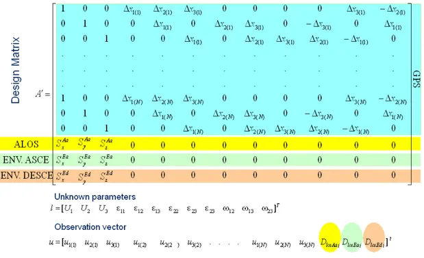
estimation problem can be expressed in the usual form Al=u+e where the coefficient matrix A assumes the following structure:

                                ∆ − ∆ ∆ ∆ ∆ ∆ ∆ − ∆ ∆ ∆ ∆ − ∆ ∆ ∆ ∆ ∆ − ∆ ∆ ∆ ∆ ∆ ∆ − ∆ ∆ ∆ ∆ − ∆ ∆ ∆ ∆ = 0 0 0 0 0 0 0 0 0 0 0 0 0 1 0 0 0 0 0 0 0 1 0 0 0 0 0 0 0 1 . . . . . . . . . . . . . . . . . . . . . . . . . . . . . . . . . . . . 0 0 0 0 1 0 0 0 0 0 0 0 1 0 0 0 0 0 0 0 1 ) ( 1 ) ( 2 ) ( 3 ) ( 2 ) ( 1 ) ( 1 ) ( 3 ) ( 3 ) ( 2 ) ( 1 ) ( 2 ) ( 3 ) ( 3 ) ( 2 ) ( 1 ) 1 ( 1 ) 1 ( 2 ) 1 ( 3 ) 1 ( 2 ) 1 ( 1 ) 1 ( 1 ) 1 ( 3 ) 1 ( 3 ) 1 ( 2 ) 1 ( 1 ) 1 ( 2 ) 1 ( 3 ) 1 ( 3 ) 1 ( 2 ) 1 ( 1 P z P y P x N N N N N N N N N N N N N N N S S S x x x x x x x x x x x x x x x x x x x x x x x x x x x x x x A ( 8)

While the measured data vector assumes the form:

u

=

[

u

₁₍₁₎

u

₂₍₁₎

u

₃₍₁₎

...

u

_1(n)

u

_2(n)

u

_3(n)

D

_LOSP

]

T (9)

It should be observed that the A matrix consists of 3N+1 rows: the first 3N rows can be viewed as N blocks of three equations which represent information on the GPS position of each single EP with respect to the arbitrary point P, while the last equation refers to the corresponding DInSAR data. The interested reader can verify that expressions (8) and (9) have been resembled from those given by [25], which refers to the GPS measure only.

We emphasize that the SISTEM method is a point-wise oriented approach. This means that, at the unknown point P, SISTEM solves the WLS problem by taking into account the surrounding GPS points and only the DInSAR data coincident with the point P. Therefore the spatial correlation of DInSAR data is not taken into account. Finally, the point-wise approach

implies that for areas where DInSAR data is missed (e.g. low coherency, decorrelated areas, etc.) the SISTEM does not provide the integrated deformations.

In order to solve the problem by using the WLS method it is necessary to modify the covariance matrix structure of observation by adding the variance of DInSAR data points. For this purpose we estimated the variance of the DInSAR data directly from the interferogram by using a sample semi-variogram γ(hc) (eq. 10) [30, 31]

[

]

2 1 ) ( ) ( 2 1 ) (

∑

= − = N i i i c d r d s N h

γ

(10)

where hc is a classified separation distance.

The weight function (7) has been used only on GPS data, because for each arbitrary point P the D_LOSP measurement is known.

In this method, the only parameter that needs to be appropriately chosen is the parameter d0 in order to define the level of locality of the estimation. As suggested by [26] we have related d0 with the mean inter-distance between neighbour stations. In particular let N be the number of EPs point of the network and Ki be the set of M nearest stations in the circle centered at the i station. It is obvious that the radius of this circle depends on i. We propose the following empirical formula to evaluate d0:

∑∑

= ∈ = N i j K ij i d NM d 1 0 1 (11)

The optimal value of M depends on the topology of the network; based on several trials, we have empirically found that for random configurations M ranges between 4 and 6.

It should be noted that the effects of the locality d0 are the following: only the points closer than about d0 to P give a significant contribution to its estimation; the uniform distribution of the strain is required only in a neighbourhood of each computation point; for points P far away the EPs the DInSAR data becomes the dominant information source.

In order to estimate the goodness of the SISTEM method, we have used the estimated standard error provided by the WLS approach.

A Synthetic case study

The SISTEM method is firstly tested on synthetic interferograms and displacement fields obtained by assuming a specific strain pattern and by using a synthetic topography. As proposed by [9]; the topography is computed according with

z

( )

x,y =z₀e−

(

(

x2+y2

)

/w

)

(12) where z(x,y) is the elevation at a point {x,y}, z0 is the initial maximum elevation to the central point, and w is a form factor used to adjust the slope and the size of the hill (Fig.1). In our case z0 =1000 m and w =1.

The synthetic dataset was generated by assuming a point pressure source [18, 1] (Mogi, 1958; Dzurisin, 2007) defined by:

(

)

                  − ∆ =           3 3 2 3 1 3 3 2 1 1 R d R x R x P a u u u µ ν (13)

Where uj (j=1,3) are the displacements along the three directions estimated at the point P (x1,

x2, d), -d is the depth of the pressure source and 22 2 2

1 x d

x

R= + + is the radial distance of

the point P from the centre of the pressure source; ν and µ are the Lame’s constants. The pressure source was embedded in an elastic homogeneous Poissonian half-space (Poisson’s ratio = 0.25, i.e. λ = µ), and, to take into account the effect of the topography, the simple varying-depth model proposed by [32] was adopted, which consists of assuming a different -d at each computation point.

Through the tests the pressure source was centred on a 400x450 grid (cell-size 100 m x 100 m) with µ=30 GPa, depth = 5000 m (with respect to the base of the topography) and with a “strength” parameter (a3∆P ) = 1017 Pa*m3. The synthetic data set consists of the 3D displacements computed at the EPs and the synthetic interferogram relevant to the considered domain (40 km x 45 km). In the tests we consider the EPs as GPS stations. A Gaussian noise of a form N=(0, σ=5 mm) and N=(0, σ=10 mm) for the horizontal and vertical components respectively were added to the GPS synthetic data. Referring the DInSAR synthetic data, in order to be as realistic as possible we have added a spatial correlated noise with a variance of 3mm calculated on the basis of a fixed covariance matrix by assuming an exponential decay with scale length of 500 meters [33].

In order to estimate the covariance matrix of the synthetic GPS points we have firstly generated a time series representing the pressure value of the Mogi source in the range 0-1017 Pa*m3 at different time instants. This was necessary since the original Mogi model is a static one. According with expression (13) we generated three time series u1(t), u2(t) and u3(t) to evaluate the covariance matrix of the synthetic data set.

Fig. 2 reports the results of the test obtained by using 100 Experimental Points (EP) randomly located assuming a locality (d0) of 2000 m..

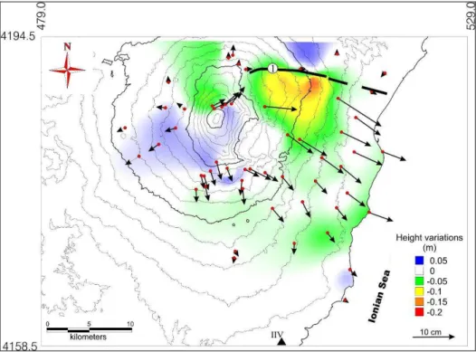
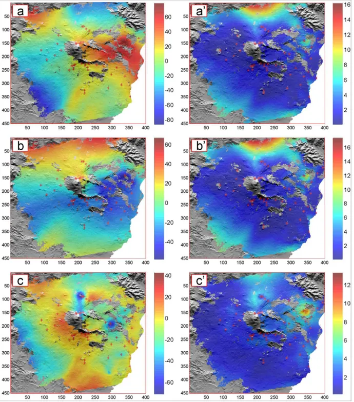
Figure.2 In the frames a,b,c are reported respectively the East, North and Up components of the displacement

field while on the frame d is reported the LOS generated on the synthetic topography; the frames a, b, c and d are obtained by using the Mogi source (no error added). The frames e, f, g and h represent the three displacement components and the LOS displacements calculated by SISTEM integration method (for details see the text). In the frames i, l, m and n are reported the residuals of the East, North, Up components and LOS respectively. In the lower row are reported the normalized histograms of the corresponding residual errors, the mean value (µ) and standard deviation (σ).The red point represents the locations of the EPs used for integration. All reported values are in mm.

The original horizontal displacement components have a symmetric shape and range from -30 mm to 30 mm, while the vertical component is very steep at the center area, where it reaches a maximum of about 70 mm.

The components of the displacements calculated by the proposed method are in good agreement with the original data and produce residuals between ±6mm for all the components. The highest residuals are generally localized in areas where both the density of EPs is low and the magnitude of expected deformations is high. The residuals of the vertical component are lower than those relevant to the horizontal ones. The pattern of the residuals of the LOS displacements is peculiar showing a ring-shape feature, around the center area of the image, with the highest residuals on the steepest slopes of the topography. Apart from the scarcity of EPs in these areas, at the origin of this peculiar feature it should be the effect of the difference in considering the distances among points between the models used for computing the synthetic data set [18, 19] and the SISTEM. [32, 34] are, indeed, intrinsically planar, i.e. the distances among points are computed as horizontal, while SISTEM is intrinsically 3D; this difference may produce severe effect on steepest slopes. In order to avoid similar artifacts, in future works we will test the correction proposed by [35], which is more precise than that proposed by [32], but it is more complex and requires more computation time.

The distributions of the errors, reported in the last row of Fig. 2, are slightly biased for all 3D component, but not for the LOS deformations. The reason of such a behavior is due to the random distribution of the EPs. Indeed, by performing a huge number of experiments we found that the best performance is obtained when a regular grid of GPS point is considered. This is rather obvious and has been pointed out by other authors [36]. However, since we think that the random distribution of EPs depicts the actual cases more than a regular distribution, we prefer to maintain these results, even if biased.

Although the integration of DinSAR and GPS data for obtaining the 3D displacement maps is the primary goal of this work, we emphasize that another important issue of the SISTEM

methodology is to provide the strain tensor components (ε11 ε12 ε13 ε22 ε23 ε33 ) and the body rotation tensor (ω1 ω2 ω3 ) .

For simplicity we show the three meaningful invariants of the 3D strain field [37]: the “dilatation”, the “differential rotation magnitude” and the maximum shear strain” (see Fig.3). The dilatation is the only linear invariant and it is defined as follows:

∑

= = n i ii n ₁ 1 ε σ (14)

where εii are the diagonal elements of the strain tensor matrix (2). The differential rotation magnitude invariant is a quadratic invariant and it is given by the following expression:

32 2 2 2 1 2 ₌

ω

₊

ω

₊

ω

Ω (15)

Finally the maximum shear strain is given by

M

=

λ

max

−

λ

min (16)

where λmax and λmin are respectively the largest and the smallest eigenvalues of the strain tensor matrix (2).

The shape and magnitude of the three invariants are in agreement with the Mogi source adopted for this synthetic case.

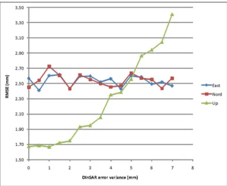
A further aim of the synthetic test is to investigate the distribution of RMSE as a function of the number of EPs considered in the range of 12 to 150. In order to assess from the statistical point of view the RMSE we have performed an appropriate number of simulations. In particular we have considered the following sequence of points: 12,20,30, … , 140, 150. For a fixed number of EP we have randomly generated 5000 different configurations of EP in the rectangular domain considered and evaluated the corresponding locality parameter d0. This means that for a fixed number of EPs a range of values is obtained as show in Fig. 4. As obvious for increasing number of EP both the range and the mean values of d0 decreases.

Figure.3 Strain invariants for the synthetic case study. The “dilatation” (a) , the “differential rotation

Figure.4 Locality (d0) in meter vs. number of Experimental Points (EPs), for the synthetic case of study. The

d0 value is calculated using 5000 random configurations, for each number of EPs, on an area of 2000 Km2,

according to the equation (11).

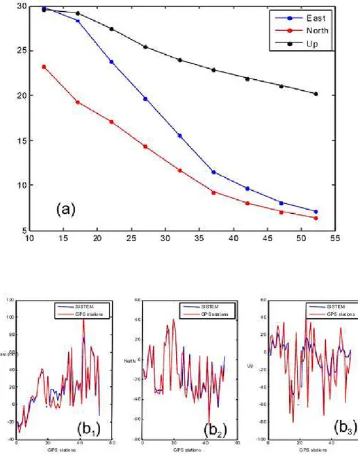
The behavior of the RMSE vs the number of EP is reported in Fig. 5. It is possible to see that, as expected, the RMSE decreases (and thus the accuracy of the method increases) as the number of EP point increases. However the plateau visible in Fig. 5 suggests that in the considered synthetic case study a good trade-off between accuracy and number of EPs can be obtained by using 50-60 EPs. Indeed, for a number of EPs greater than 50-60 there are no significant improvement of the performance. We highlight that the magnitude of the RMSE are comparable with those reported by [9, 38].