Micromagnetic modeling of spintronic devices: from uniform state to skyrmion

Dottorato di Ricerca in

Ingegneria dei Sistemi ed Informatica

CICLO

XXVIII

Modellizzazione micromagnetica di dispositivi

spintronici: dallo stato uniforme allo skyrmion

Settore Scientifico Disciplinare ING-IND/31

Coordinatore: Ch.mo Prof. Felice Crupi

Firma ____________________

Supervisore: Ch.mo Prof. Mario Carpentieri

Firma______________________

Dottorando: Dott. Riccardo Tomasello

Degree of Doctor of Philosophy in

System and Computer Engineering

CYCLE

XXVIII

Micromagnetic modeling of spintronic devices: from

uniform state to skyrmion

Scientific Sector ING-IND/31

Coordinator: Ch.mo Prof. Felice Crupi

Firma ____________________

Supervisor: Ch.mo Prof. Mario Carpentieri

Firma______________________

Ph. D. student: Dott. Riccardo Tomasello

i

RIASSUNTO

La Spintronica è una branca della Fisica che ha attratto un notevole interesse negli ultimi 30 anni. Diversamente dall’Elettronica, che affida alla carica dell’elettrone la codifica binaria, la Spintronica prende in considerazione sia la carica sia il momento di spin degli elettroni. Tale connubio tra carica e spin consente agli spin di influenzare il trasporto degli elettroni, e, viceversa, alle cariche elettriche di modificare le proprietà magnetiche. In questo modo, si sono resi possibili la progettazione e fabbricazione di dispositivi caratterizzati da dimensioni nanometriche, basso consumo di energia, non-volatilità, alta velocità, grande scalabilità e compatibilità con l’odierna industria elettronica.

I dispositivi spintronici sono tipicamente composti da un tristato dove un materiale non magnetico è frapposto tra due ferromagneti. La magnetizzazione di uno di essi può essere manipolata, non soltanto tramite l’applicazione di campi esterni, bensì anche per mezzo di una corrente elettrica che fluisce perpendicolarmente al multistrato. Questo grado di libertà aggiuntivo nel controllo delle dinamiche della magnetizzazione ha dato vita a molteplici applicazioni tecnologiche dei dispositivi spintronici, come memorie magnetiche, le quali sono state già commercializzate, oscillatori alle frequenze delle microonde, che sono gli oscillatori più piccoli esistenti in natura, e rilevatori a microonde, la cui sensitività ha già superato quella dei diodi Schottky.

Una strategia per migliorare le prestazioni dei dispositivi spintronici concerne l’uso di configurazioni non uniformi della magnetizzazione, tra le quali gli skyrmion hanno mostrato caratteristiche promettenti. La principale peculiarità è la protezione topologica, che rende gli skyrmion molto stabili e difficili da essere distrutti.

Questa tesi descrive i risultati ottenuti mediante simulazioni micromagnetiche sulle memorie magnetiche, oscillatori e rivelatori alle frequenze delle microonde basati sia sullo stato uniforme della magnetizzazione, sia sullo skyrmion.

ii Spintronics is a branch of Physics which has attracted a lot interest over the past 30 years. Differently from Electronics, that entrusts the binary encode to the electron charge, Spintronics considers both charge and spin momentum of electrons. This bond between electron charge and spin allows to alter the electronic transport by spins, and, vice versa, to affect the magnetic properties by electron charges. In this way, it has been possible to design and make devices characterized by nanometer dimensions, low energy consumption, non-volatility, large speed, high scalability, and compatibility with nowadays’ electronic industry.

Spintronic devices are typically composed of a trilayer where a non-magnetic spacer is sandwiched between two ferromagnets. The magnetization of one of them can be manipulated, not only by external applied fields, but also by an electrical current perpendicularly injected into the stack. This additional degree of freedom in controlling the magnetization dynamics has given rise to several technological applications of spintronic devices, as magnetic storages, which have been already commercialized, microwave oscillators, which are the smallest oscillators existing in nature and microwave detectors, whose sensitivity has already overcome the one of Schottky diodes.

A strategy to improve the performances of spintronic devices concerns the use of non-uniform configurations of the magnetization, among them skyrmions have shown promising features. The main characteristic is the topological protection which makes skyrmions very stable and hard to be wrecked.

This thesis shows the results achieved by means of micromagnetic simulations on magnetic storages, microwave oscillators and detectors based on both a uniform and a skyrmion state of the magnetization.

iii

ACKNOWLEDGEMENTS

During my Master Degree, my colleagues and I, Angelo and Domenico, used to imagine working for a big company after graduating. However, my life did not go in the direction I expected. I attended a course on Magnetic Materials and Spintronics, taught by Prof. Giovanni Finocchio, who involved me in a deeper study of Spintronics and encouraged me to continue my studies. His first words to me were: “Riccardo, la cosa più importante è scrivere articoli!! (Riccardo, the most important thing is to write papers)”. I owe a lot to Giovanni, from his guidance, indispensable support, useful work suggestions, valuable comments on different aspects of my research to his general advices for everyday life; because, as well as being an amazing professor, he is a great man and friend. His support his essential to my success. I can still feel my enthusiasm when he proposed me to spend almost two months at the University of Irvine, California, with Prof. Ilya Krivorotov and his group. I packed my stuff, and, with the few English words I knew at that time, I travelled all the way to California by myself, without an accommodation and not knowing anyone. It was a tough and crazy experience. I took the first serious contact with the world of Research and it helped me grow personally and professionally.

When I returned from the USA, I applied for the PhD position under the supervision of Prof. Mario Carpentieri. I have learned oodles of things from him: how to organize my work, tutor students, teach classes, write a paper, and much more. He is such an excellent person, supervisor and professor. I’m fully indebted to him for his understanding, guidance, encouragement, indispensable advice and information over the last three years and for pushing me farther than I thought I could go. The only thing I’m afraid of is not being up to his standards, since his most frequent sentence is: “Riccardo, sei sempre in vacanza!!! (Riccardo, you are always on vacation)”.

Besides being grateful towards those two mentors, I’m glad to have met great educators such as Prof. Domenico Grimaldi, Prof. Luca Carnì,

iv Prof. Francesco Lamonaca, Prof. Sergio Greco, Prof. Felice Crupi and Prof. Marco Lanuzza towards whom I’m really thankful for their kindness, assistance and support.

I cannot avoid mentioning my first trip to Salamanca. I feel very privileged to have worked at the University of Salamanca under the supervision of kind and illustrious professors: Prof. Luis Torres, Prof. Eduardo Martinez and Prof. Luis Lopez-Diaz, and, more in general, I’m very happy and grateful to have been in Salamanca. I spent one of the most wonderful periods of my life there, both from a work achievement point of view and from a life-experience one. For this reason, I want to also thank all my Salamanca friends, especially my best friend David, Vincent, and Ignacio, as well as all the members of the group “Addicts to O’hara’s”.

I also want to acknowledge Prof. Ozhan Ozatay and his group (especially Vedat and Aisha) for the beautiful time spent at Bogazici University in the magic and chaotic Istanbul.

Another important step for my career and experience has been my attendance at the Magnetics Summer School in Minneapolis, Minnesota, which made me very proud of my research achievements since I was the only PhD student from Italy there.

Let’s rewind to the beginning, because all this would have not been possible without meeting the charismatic Prof. Bruno Azzerboni and his fabulous group, above all my friends Vito and Anna, and the meticulous Giulio. It has been an honor collaborating with them and a pleasure as well, because, within this group, it is always possible to work with “a smile on your face”. In Prof. Azzerboni words: “Tenete alto il nome del gruppo divertendovi!”(Keep high the name of the group, having fun).

I also express my deep sense of gratitude to my best friend Nunzio, who has always been by my side supporting me (i.e. He accompanied me for the admission exam for the PhD) and of course my amazing parents, for their co-operation, understanding and constant encouragement which were the sustaining factors to carry out this work successfully. Thank you, mom and dad, for your support, for giving me strength and your love, throughout

v my studies in all the ways possible. I hope this thesis would be a worthy reward for what you have done for me.

Lastly, it is my privilege to conclude the acknowledgments mentioning my girlfriend, who is the most important gift Salamanca has given me. I am extremely thankful for her constant support and encouragement throughout my research period and for helping me improve my English. I hope to continue sharing my life with her for a long time.

vi

1. BASIC CONCEPTS ... 1

1.1 Micromagnetism ... 1

1.1.1 Exchange energy ... 3

1.1.2 Uniaxial Anisotropy energy ... 3

1.1.3 Magnetostatic energy... 4

1.1.4 Zeeman energy ... 6

1.2 Equilibrium and dynamical equations ... 7

1.2.1 Oersted Field ... 8 1.2.2 Thermal Field ... 8 1.2.3 Dynamical equation ... 9 1.2.4 Spin-Transfer Torque... 11 1.2.5 STT in OOP devices ... 12 1.2.6 STT in IP devices ... 14

1.2.7 Voltage controlled magnetocrystalline anisotropy (VCMA) ... 15

1.3 Spin-orbit interactions ... 16

1.3.1 Spin-Hall Effect ... 19

1.3.2 Rashba effect ... 21

1.3.3 Dzyaloshinskii-Moriya Interaction ... 22

1.3.4 Three terminal MTJ device ... 23

1.4 Magnetic skyrmions ... 24

1.4.1 Topology and skyrmion number ... 25

1.4.2 Observations of skyrmions ... 27

vii

2.1 MTJ based STT-MRAM ... 29

2.1.1 Tunnel MagnetoResistance ... 30

2.1.2 Writing and reading process ... 32

2.1.3 Thermal stability and writing energy ... 34

2.1.4 State of the art ... 35

2.1.5 Comparison with other technologies ... 37

2.2 Results on STT-MRAMs ... 39

2.2.1 Switching Properties in Magnetic Tunnel Junctions With Interfacial Perpendicular Anisotropy: Micromagnetic Study ... 39

2.2.2 Micromagnetic Study of Electrical-Field-Assisted Magnetization Switching in MTJ Devices ... 47

2.3 Racetrack memory ... 55

2.4 Results on racetrack memories ... 57

2.4.1 A strategy for the design of skyrmion racetrack memories ... 57

3. SPIN-TORQUE OSCILLATORS AND DIODES ... 67

3.1 Introduction on oscillators ... 67

3.2 Spin-torque nano-oscillators ... 69

3.2.1 Classification of STNOs ... 70

3.2.2 State of the art ... 74

3.3 Results on STNOs ... 76

3.3.1 Dynamical properties of three terminal magnetic tunnel junctions: spintronics meets spin-orbitronics ... 76

3.3.2 Intrinsic synchronization of an array of spin-torque oscillators driven by the spin-Hall effect ... 83

3.4 Spin-torque diode ... 87

viii

3.4.2 State of the art ... 90

3.5 Results on Spin Torque Diode ... 92

3.5.1 Influence of the Dzyaloshinskii-Moriya interaction on the spin-torque diode effect ... 92

4. SPIN-TORQUE OSCILLATOR AND DIODE BASED ON SKYRMION ... 97

4.1 Topological, non-topological and instanton droplets driven by STT in materials with perpendicular magnetic anisotropy and DMI ... 97

4.2 Skyrmion based microwave detectors and harvesting ... 107

5. JOURNAL ARTICLES... 116

5.1 Published articles ... 116

5.2 Submitted articles ... 118

ix

LIST OF ABBREVIATIONS

AHE Anomalous Hall Effect;

AMR Anisotropic Magnetoresistance;

AP Antiparallel;

AV Anti-Vortex;

BC Boundary conditions

BIA Bulk Inversion Asymmetry;

CMOS Complementary Metal-Oxide Semiconductor;

DMI Dzyaloshinskii-Moriya Interaction;

DRAM Dynamic Random Access Memory;

DW Domain-Wall;

FM Ferromagnetic;

FMR Ferromagnetic Resonance;

FWHM Full Width at Half Maximum;

GMR Giant MagnetoResistance:

HM Heavy Metal;

ID Instanton Droplet;

i-DMI Interfacial Dzyaloshinskii-Moriya Interaction;

IP In-Plane;

IPA Interfacial Perpendicular Anisotropy;

LLG Landau-Lifshitz-Gilbert;

LLGS Landau-Lifshitz-Gilbert-Slonczewski;

MRAM Magnetic Random Access Memory;

MSMDMT Micromagnetic Spectral Mode Decomposition Mapping Technique;

MTJ Magnetic Tunnel Junction;

MWS Micromagnetic Wavelet Scalogram;

NTD Non Topological Droplet;

x

P Parallel;

SCD Switching Current Density;

SHE Spin-Hall Effect;

SIA Structural Inversion Asymmetry;

SMD Spatial Mode Distribution;

SOC Spin-Orbit Coupling;

SOT Spin-Orbit Torque;

SRAM Static Random Access Memory;

SS Static Skyrmion;

STD Spin-Torque Diode;

STNO Spin-Torque Nano-Oscillator;

STT Spin-Transfer-Torque;

STT-MRAM Spin-Transfer-Torque-Magnetic Random Access Memory;

TD Topological Droplet;

TMR Tunnel MagnetoResistance;

V Vortex;

VCMA Voltage Controlled Magnetocrystalline Anisotropy;

xi

LIST OF SYMBOLS

dV volume of magnetic material;

r vector position;

M magnetization vector;

MS saturation magnetization;

 spin angular momentum;

m normalized magnetization vector;

ex

 exchange energy density;

A exchange constant;

mx x-component of the normalized magnetization;

my y-component of the normalized magnetization;

mz z-component of the normalized magnetization; an

 uniaxial anisotropy energy density;

1

k or ku first order uniaxial anisotropy constant;

2

k second order uniaxial anisotropy constant;

3

k third order uniaxial anisotropy constant;

k

u unit vector of the magnetization easy axis;

Hm magnetostatic field;

B magnetic induction;

0 vacuum permeability;

m

  volume magnetic charge density;

m

U scalar potential;

n normal unit vector;

( )

m r

 surface magnetic charge density;

m

 magnetostatic energy density;

Nx x-axis shape-dependent demagnetizing factor;

xii

Nz z-axis shape-dependent demagnetizing factor;

Hext external magnetic field; ext

 external magnetic field energy density;

tot

 total energy density of a ferromagnetic body;

eff

H effective field;

eff

h normalized effective field;

HOe Oersted field;

T material temperature;

Hth stochastic thermal field;

KB Boltzmann constant;

ΔV volume of the computational cell;

Δt simulation time step;

 three-dimensional white Gaussian noise;

 torque;

L orbital angular momentum;

 gyromagnetic ratio; g Landé factor; e electron charge; me electron mass; B Bohr magneton;  Planck’s constant;

 damping parameter or Gilbert damping;

FE-oop

j or J  perpendicular current density;

JMTJ perpendicular current density in MTJ;

p

m normalized magnetization of the pinned layer;

f

m normalized magnetization of the free layer;

oop

τ STT in OOP device;

xiii

( , )

 m mf p polarization function; ( , )

SV m mf p

 polarization function for spin-valve;

 spin polarization factor for OOP device;

( , )

MTJ m mf p 



polarization function for MTJ;

d dimensionless time step;

FE-ip

j or jFE IP current density through ferromagnet; a

IP

τ adiabatic torque for IP device;

P spin polarization factor for IP device;

na

IP

τ non-adiabatic torque for IP device;

 non-adiabatic parameter;



k

H perpendicular anisotropy field;

Vapp applied voltage;

HSO Spin-orbit Hamiltonian; ( ) V r electrical potential; SHE τ SHE torque; SH  spin-Hall angle;

jHM charge current density through a HM; s

j spin current;

hR Rashba effective field;

R Rashba torque;

R

  Rashba parameter;

BulkDMI

 Bulk DMI energy density;

D DMI parameter;

InterDMI

 Interfacial DMI energy density;

 DMI characteristic length;

xiv

RP Parallel electrical resistance of OOP device;

RAP AP electrical resistance of OOP device;

JC switching current density;

ip C

J switching current density for IP MTJ;

k

H anisotropy field;

oop C

J switching current density for OOP MTJ;

I electrical current;

 thermal stability factor;

keff effective anisotropy constant;

V magnetic volume of ferromagnet;

Keff

H effective anisotropy field;

Ew write energy;

tp current pulse width;

S cross section of the free layer;

l length or diameter of a ferromagnet (or free layer cross section);

hIPA IPA effective field contribution;

dt time step;

<m> average normalized magnetization;

G gyrocoupling vector;

x

v x-component of the velocity of DW or skyrmion;

y

v _{y-component of the velocity of DW or skyrmion;}

D dissipative tensor;

R IP rotation matrix;

Dg roughness size;

Δy2 y-position of a skyrmion in a racetrack memory;

w ferromagnet width;

x1 travelling x-distance of a skyrmion in a racetrack memory; p

xv

out

P or pout output power;

in

P input power;

Q quality factor;

0

f FMR frequency;

R electric resistance of an OOP device;

m

R average resistance value;

R

 orR_S amplitude of the oscillating resistance;

 angular frequency;

 intrinsic phase shift;

out

V or vout output voltage;

L

R resistance of an inductive load;

max

M amplitude of the magnetization oscillation;

Jth Threshold current density for persistent magnetization oscillations;

jMTJrf perpendicular microwave current density in MTJ; MAX

J perpendicular microwave current density amplitude in MTJ;

rf

f perpendicular microwave current density frequency in MTJ;

L locking range;

S

  synchronization angular frequency;

M

V amplitude of the applied voltage;

R0 resistance load;

i

G conductance of i-MTJ;

,i

m

G average conductance value of i-MTJ;

i

G

 amplitude of the conductance of i-MTJ;

tHM thickness of HM;

MTJrf

i _{perpendicular microwave current in MTJ;}

I

xvi

R

 intrinsic phase shift of R;

dc V dc output voltage; S  phase difference;  diode sensitivity; dc contact diameter; c

D critical i-DMI parameter;

min

r minimum radius of the skyrmion;

max

r maximum radius of the skyrmion;

c

r contact radius;

dSK skyrmion diameter;

dSK-min minimum diameter of the skyrmion;

dSK-max maximum diameter of the skyrmion;

VCMA

H VCMA effective field contribution;

VCMA H

xvii

LIST OF FIGURES

Fig. 1.1: fundamental assumption of Micromagnetics, by which the magnetic momenta μi of a volume element dV can be represented by a magnetization vector M. ... 3 Fig. 1.2: (a) persistent precession of the magnetization Maround the effective field Heffwhen only the conservative torque acts. (b) Damped precession of the magnetization when the damping torque is considered. .. 10 Fig. 1.3: schematic representation of the creation of the spin-polarized current. Part of the entering spins in the ferromagnet1 are polarized in the same direction of M1, generating the spin-polarized current, which will transfer a spin-torque onto the magnetization M₂ of the adjacent ferromagnet2. Part of the entering spins is reflected with a polarization opposite to M1. ... 11

Fig. 1.4: (a) schematic illustration of the spin-transfer torque exerted on the free layer magnetization in an OOP device. (b) representation of all the torques acting on the magnetization. ... 14 Fig. 1.5: schematic representation of two domains (UP and DOWN) separated by a domain wall. A non-polarized electron flowing through this magnetization configuration will change the direction of its spin adiabatically, namely it will follow the local magnetization orientation... 15 Fig. 1.6: variation of the effective perpendicular anisotropy field when a voltage is applied in CoFeB-MgO MTJs [29]. ... 16 Fig. 1.7: schematic picture of (a) the skew scattering mechanism and (b) the side-jump mechanism. The letters U and D refer to the sign of the spin, respectively spin-UP and spin-DOWN. The yellow circle represents an impurity... 18

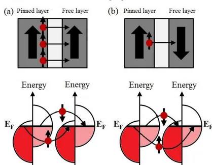
xviii Fig. 1.8: (a) example of crystalline lattice characterized by the inversion symmetry property. (b) Example of crystalline lattice lacking the inversion symmetry. ... 19 Fig. 1.9: schematic picture of the FM/HM bilayer, where the SHE arises, inducing opposite spin accumulations near the upper and lower surface of the HM. ... 19 Fig. 1.10: the Rashba effect arises in FM/HM bilayers, when the electrical current flows through the ferromagnet. ... 21 Fig. 1.11: (a) bulk DMI vector originating in a non-centrosymmetric crystal because of the interaction of the ferromagnetic atoms with an impurity with large SOC. (b) Interfacial DMI vector in a FM/HM bilayer. ... 22 Fig. 1.12: schematic representation of a three terminal device, where an MTJ is coupled through its free layer to a HM underlayer... 24 Fig. 1.13: magnetization configurations with skyrmion number S equal to (a) zero, (b) one, and (c) two [54]. ... 26 Fig. 1.14: magnetization distribution of a (a) Bloch skyrmion and (b) Néel skyrmion [47]... 27 Fig. 2.1: schematic illustration of the TMR phenomenon in MTJs, where in (a) the magnetization state is parallel, allowing many spin-UP electrons to tunnel from the pinned layer to the free layer, in (b) the magnetization state is AP and just few spin-UP electrons can tunnel, leading to a high resistance of the MTJ. In the bottom panels, the density of states at Fermi level are represented, corresponding to the two ferromagnets in the two magnetization configurations... 31 Fig. 2.2: schematic representation of a MTJ connected in series with a selection transistor. ... 33 Fig. 2.3: schematic illustration of (a) an IP MTJ and (b) an OOP one. ... 34 Fig. 2.4: schematic representation of the studied MTJ. ... 40

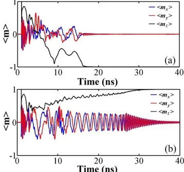
xix Fig. 2.5: IP SCD depending on the perpendicular anisotropy. The three curves with symbols refer to a saturation magnetization equal to 8x105 A/m, 10x105 A/m and 12x105A/m. The green line without symbols represents the minimum values of IPA over which, for a fixed MS, the free layer is OOP. ... 41 Fig. 2.6: representation of the spin magnetization domains of the MTJ elliptical section, describing the IP switching phenomenon, when the spins are oriented along (a) -x and (c) x and (b) during the switching... 42 Fig. 2.7: IP SCD as function of the perpendicular anisotropy, without the Oersted field. The two curves refer to a saturation magnetization equal to 10x105 A/m and 12x105A/m. ... 43 Fig. 2.8: IP SCD depending on the perpendicular anisotropy, without the Oersted field and for a reversal time of 10 ns The three curves refer to a saturation magnetization equal to 8x105 A/m, 10x105 A/m and 12x105A/m. ... 43 Fig. 2.9: OOP SCD as function of the perpendicular anisotropy, for a switching time of (a) 10 ns and (b) 5 ns. The curves refer to a saturation magnetization equal to 8x105 A/m, 10x105 A/m and 12x105 A/m. ... 44 Fig. 2.10: IP SCD as function of the perpendicular anisotropy, without the Oersted field and for a reversal time of 20 ns at a temperature T=350 K. The three curves refer to a saturation magnetization equal to 8x105 A/m, 10x105 A/m and 12x105A/m. ... 45 Fig. 2.11: switching averaged energy as function of the IPA for (a) the IP switching, (b) OOP switching in 10 ns and (c) OOP switching in 5 ns. ... 46 Fig. 2.12: Sketch of the studied MTJ device. ... 49 Fig. 2.13: (a) applied current pulses. (b) Time domain plot of the three normalized components of the magnetization (<mx>, <my> and <mz>, respectively represented in blue, red and black) during a whole reversal process (PAP and APP) as a function of the current pulses in (a). ... 50

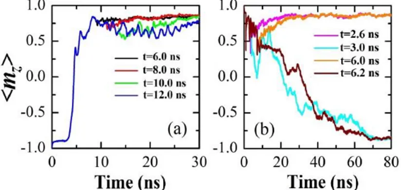
xx Fig. 2.14: time domain plot for the three normalized components of the magnetization <mx>, <my> and <mz>, respectively represented in blue, red and black. (a) Pulse time of 3 ns. (b) Pulse time of 2.6 ns. ... 51 Fig. 2.15: spatial magnetization configurations before the current pulse is switched off. The arrows refer to the y-component of the magnetization (blue positive and red negative), whereas the background colors refer to the

z-component (red positive direction and blue negative direction). The letter

“V” indicates vortexes, while “AV” refers to antivortexes. (a) Pulse time of 3 ns. (b) Pulse time of 2.8 ns. (c) Pulse time of 2.6 ns. (d) Pulse time of 3.4 ns. (e) Spatial magnetization configuration after the current pulse is removed for a pulse time (e) t=3 ns and (f) t=2.6 ns. ... 53 Fig. 2.16: time domain plot for the z-component of the magnetization for different time pulses at T=300 K. (a) PAP switching process. (b) APP switching process. ... 54 Fig. 2.17: evolution of DW racetrack memory. (a) and (b) represent a single ferromagnetic wire with IP and OOP domains, respectively. (c) bilayer where the DW motion is induced by the SHE. (d) motion of DWs due to the SHE in a synthetic antiferromagnet. ... 56 Fig. 2.18: (a) Néel skyrmion motion driven by the STT. (b) Néel skyrmion motion driven by the SHE. (c) Bloch skyrmion motion driven by the STT. (d) Bloch skyrmion motion driven by the SHE. The four insets show the spatial distribution of the Néel and Bloch skyrmion, where the background colors refer to the z-component of the magnetization (blue negative, red positive), while the arrows are related to the IP components of the magnetization. The current flows along the x-direction. The skyrmion moves along the x-direction in the scenarios A, C, and D and along the y-direction in the scenario B. ... 58 Fig. 2.19: (a) A comparison among the skyrmion velocities obtained for each scenario (A, B, C, and D). The current jFE is related to the scenarios A

xxi and C while jHM to the scenarios B and D. (b) Sketch of the motion mechanism of the Néel skyrmion driven by the SHE along the y-direction. (c) Sketch of the motion mechanism of the Bloch skyrmion driven by the SHE along the x-direction. (d) Skyrmion velocities as a function of jHM obtained for the scenario B: (i) thermal fluctuations (T=350 K) and perfect strip (red curve) and (ii) thermal fluctuations (T=350 K) and rough strip (blue curve). The arrows for (b) and (c) refer to the IP components of the magnetization, the spin-polarization of jHM is also displayed. ... 61 Fig. 2.20: (a) phase diagram (i-DMI parameter vs. external field) of the skyrmion stability. The colored part highlights the region where the skyrmion is stable and the red curve points out the values of D and Hext for which the skyrmion diameter is 46 nm. (b) Skyrmion velocity as a function of the current calculated by micromagnetic (black curve) and analytical computations (green line). (c) Time domain evolution of the skyrmion diameter during the transient breathing mode at three different values of the

jHM, 30 MA/cm2 (black curve), 40 MA/cm2 (blue curve) and 50 A/cm2 (red curve). (d) A comparison of skyrmion velocity as a function of the current for an ideal strip (T=0K) and a rough strip and room temperature. ... 63 Fig. 2.21: (a) sketch of the skyrmion motion due to the SHE in a sample confined along the y-direction. (b) Skyrmion velocity (x-direction) as a function of the current: (i) no thermal fluctuations and perfect strip (red curve) and (ii) thermal fluctuations (T=350 K) and rough strip (black curve). (c) Skyrmion velocity as a function of the current when the strip width w is 100 nm (red curve), 150 nm (black curve) and 200 nm (blue curve). The colors for (a) refer to the z-component of the magnetization (blue negative, red positive). ... 65 Fig. 3.1: (a) schematic illustration of an STNO. (b) example of time domain oscillation of the STNO electrical resistance, when precessions of the free layer magnetization are excited. ... 70

xxii Fig. 3.2: (a) and (b) geometry classification of STNOs, (a) nanopillars and (b) nano-contact. (c), (d) and (e) magnetization configuration classification of STNOs, (c) in-plane, (d) perpendicular and (e) in-plane-perpendicular. 71 Fig. 3.3: example of MTJ-based nanopillar STNO spectra showing a narrow linewidth at room temperature [23]. ... 74 Fig. 3.4: schematic representation of the three terminal MTJ device. ... 78 Fig. 3.5: (a) oscillation frequency of the magnetization as a function of the

jHM for Hext=40 mT (top curve) and Hext=30 mT (bottom curve) when the

JMTJ is zero. (b) Temporal evolution of the three normalized components of the magnetization <mx> (dashed curve), <my> (solid curve), <mz> (dotted curve) during 1 ns of the magnetization oscillations, for jHM =-2.13x108 A/cm2, Hext=30 mT. (c) Snapshots of the magnetization during an oscillation period in the time instants reported in Fig. 3.5(b). The color scale refers to the y-component of the magnetization (red positive, blue negative). The arrows indicate the magnetization direction. ... 79 Fig. 3.6: (a) oscillation frequency for fixed Hext=30 mT and jHM =-2.13 x 108 A/cm2 as function of the bias JMTJ. (b) Fourier spectra for different values of the JMTJ. (c) Arnold tongues showing the locking regions as function of JMAX for T=0 K (lower curve) and T=300 K (upper curve) at jHM=-2.13 x 108 A/cm2. ... 80 Fig. 3.7: (a) schematic representation of the proposed highly scalable synchronization scheme. (b) Locking ranges as a function of the cross-section dimensions for JMAX=2.0 x 106 A/cm2 and jHM =-2.13 x 108 A/cm2. 83 Fig. 3.8: schematic representation of the FM/HM bi-layered device. (Inset) Detailed sketch of the bylayer structure showing the thicknesses of the layers, the direction of the current density jHM and the applied external magnetic field Hext. ... 84 Fig. 3.9: Fourier spectra as a function of jHM. (a) Hext=80 mT. (b) Hext=90 mT. ... 85

xxiii Fig. 3.10: Fourier spectra as a function of Hext. (a) jHM=-0.90x108 A/cm2, (b)

jHM=-1.00x108 A/cm2. ... 86 Fig. 3.11: MWS for Hext=90 mT, where the power increases from white to black. (a) jHM=-0.90x108 A/cm2, (b) jHM=-1.00x108 A/cm2. Insets: SMDs related to the x component of the magnetization (the power increases from white to red). ... 87 Fig. 3.12: schematic representation of an STD working in the (a) IP regime and (b) in the OOP regime. ... 90 Fig. 3.13: comparison of STD sensitivities with the one of the Schottky diode [190]. ... 91 Fig. 3.14: FMR responses for jHM=0 A/cm2. a) JMAX=0.5x106 A/cm2 without

i-DMI (top curve) and with i-DMI (bottom curve); b) JMAX=0.1x106 A/cm2 with no i-DMI (upper curve) and with i-DMI (lower curve). The insets represent the SMDs for the y- and z- components of the magnetization. .... 94 Fig. 3.15: FMR responses for a sub-critical jHM=-1.50x107 A/cm2 and a

JMAX=0.5x106 A/cm2 without i-DMI (top curve) and with i-DMI (bottom curve). The insets represent the SMDs for the y- and z- components of the magnetization. ... 94 Fig. 3.16: FMR responses for jHM=-1.40x108 A/cm2. a) JMAX=0.5x106 A/cm2 without i-DMI (top curve) and with i-DMI (bottom curve); b) JMAX=0.1x106 A/cm2 with no i-DMI (upper curve) and with i-DMI (lower curve). The insets represent the SMDs for the y- and z- components of the magnetization. ... 95 Fig. 4.1: spin valve with a point contact geometry, where the Co free layer is coupled to the Pt underlayer. For the sake of clarity, an enlarged view of the nanocontact (fixed layer) and the diameter dc of the nanocontact are illustrated, together with the dimensions l  l of the square cross section. . 99

Fig. 4.2: (a) stability phase diagram of the magnetization ground-state as a function of the modulus of the current density and of D at zero external

xxiv magnetic field. Letters A, B, C and D are linked to Fig. 4.4. The meaning of the symbols in the phase diagram are as follows. FM: ferromagnetic; SS: static skyrmion; TD: topological droplet; NTD: non-topological droplet, ID: instanton droplet. (b) Spatial distribution of the topological density (a color scale is represented, red +1, blue -1) for the three dynamical states NTD, TD, and ID at i-DMI values of 0.00, 2.50, and 1.25 mJ/m2, respectively. 100 Fig. 4.3: (a) frequency-current density hysteresis loop at D=2.0 mJ/m2: the black (red) arrows indicate the path where the initial state is FM (SS). (b) Output power as a function of current density for D=2.0 mJ/m2. The solid line refers to the analytical computation from Eq. (4.1), while the dotted line is determined by micromagnetic calculations. The black (red) arrows indicate the path where the initial state is FM (SS). (c) Two dimensional spatial profile of the TD for D=2.5 mJ/m2. ... 103 Fig. 4.4: frequency spectra as a function of the i-DMI, when J=8.5x107 A/cm2. Capital letters A, B, C, and D are linked to the phase diagram of Fig. 4.2. ... 104 Fig. 4.5: oscillation frequency as a function of D for J=8.5107 A/cm2. The different states are indicated. The inset shows the energy related to ID transitions as a function of D for J=8.5107 A/cm2... 105 Fig. 4.6: frequency spectra as a function of the contact diameter dc, when

J=8.5x107 A/cm2 and zero i-DMI, together with the spatial distribution of the topological density (red +1, blue -1) which corresponds to the frequency peak in the NTD dynamical state... 106 Fig. 4.7: sketch of the device under investigation. The extended CoFeB acts as free layer while the top nano-contact made by CoFeB is the current polarizer (dc is the contact diameter, l=100 nm). The Pt layer is necessary to introduce the i-DMI. ... 108 Fig. 4.8: (a) profile of the OOP component of the magnetization corresponding to the section AA', as indicated in the inset. dsx represents the

xxv skyrmion diameter. Inset: example of a snapshot of a Néel skyrmion stabilized by the i-DMI, where the arrows indicate the IP component of the magnetization while the colors are linked to the OOP component (blue negative, red positive). (b) and (c) Skyrmion diameter as computed by means of micromagnetic simulations (the radius is computed as the distance from the geometrical center of the skyrmion, where mZ=-1 to the region where mZ=0). Skyrmion diameter (b) as a function of D for ku=0.8 and 0.9 MJ/m3 and (c) as a function of ku for D=3.0 and 3.5 mJ/m2. ... 109 Fig. 4.9: (a) STD response as a function of D for ku.=0.8 MJ/m3. (b) STD response as a function of ku. for D=3.0 mJ/m2. (c) FMR frequency as a function of D for two different values of ku as indicated in the panel. (d) FMR frequency as a function of D (ku.=0.8 MJ/m3) for three different values of the cross section diameter l=75, 100, and 150 nm with the indication of the critical DMI parameter Dcrit. ... 111 Fig. 4.10:(a) sensitivity as a function of the contact diameter for different amplitudes of the microwave current as indicated in the main panel. (b) Detection voltage and microwave power as a function of the contact diameter forJMAX=1 MA/cm

2

. (c) Sensitivity as a function of the contact diameter for different microwave powers as indicated in the main panel. In both (a) and (c) an optimal contact diameter corresponding to a maximum in the sensitivity can be observed. (d) Detection voltage as a function of the contact diameter for different microwave powers. All the data reported in this figure are obtained for ku=0.8 MJ/m3 and D=3.0 mJ/m2. ... 113 Fig. 4.11: (a) amplitude of the z-component of the magnetization driven by

VCMA

H

 at JMAX=0 MA/cm

2

; (b) sensitivity as a function of the HVCMA,

considering the optimal contact diameter of Fig. 4(a) (dC=40 nm), computed for JMAX=1 and 2 MA/cm

2

. (c) Phase shift S as a function of HVCMA for

xxvi

LIST OF TABLES

xxvii

1

1. BASIC CONCEPTS

In this chapter, several aspects concerning Micromagnetics, Spintronics, Spin-Orbitronics will be reviewed, in order to provide the basic background necessary to read the results of this thesis. First of all, a brief introduction of the micromagnetic formalism (paragraph 1.1) and the torques acting onto the magnetization vector of a ferromagnetic material (paragraph 1.2) will be presented. Paragraph 1.3 will deal with the key concepts of Spin-Orbitronics and, the last paragraph 1.4 will introduce the magnetic texture of the skyrmion.

1.1 Micromagnetism

Micromagnetism is a continuum field theory [1, 2, 3] which aims at the study of static and dynamical properties of ferromagnetic particles within a mesoscopic level. In other words, the characteristic scale of investigation is larger than the atomic one (10-10 – 10-9 m), but small enough to describe the internal structure of magnetic domains and domain walls (DWs).

The history of Micromagnetics starts in 1935 with a paper by Landau and Lifshitz [4, 5] on the structure of a wall between two antiparallel (AP) domains, and continues with Brown [6, 7] and many others up to nowadays. For many years, Micromagnetics was only used to

2 determine nucleation processes of domains, domain structures properties [8] and magnetization dynamics in simple and ideal systems. However, since the middle of 1980s, with the development of large-scale computations, Micromagnetics acquired more and more importance for the possibility to investigate realistic problems which were more amenable to be compared with experimental data [9, 10].

One of the fundamental assumptions of the micromagnetic theory is that the magnetization of a volume of material dV, denoted by the vector position r, can be represented as a vector M, which is a continuous function of the position r and has a modulus MS constant in time (MS is the saturation magnetization of the material). In particular, the size of the volume dV has to be chosen big enough to contain a large number n of magnetic momenta

i, but small enough to allow the magnetization vector to smoothly change

between each volume element (Fig. 1.1). In this way, the magnetization can be locally expressed by:

 



We can also refer to the normalized magnetization vector as:

 

 

m r M r (in this thesis both notations m r

 

 

3 Fig. 1.1: fundamental assumption of Micromagnetics, by which the magnetic momenta μ_i of a volume element dV can be represented by a magnetization vector M .

1.1.1 Exchange energy

The exchange is a short-range interaction which tries to align neighboring magnetic momenta along the same direction [1, 7]. It is the basis of ferromagnetism and it has quantum-mechanical origins linked to the overlapping wave functions among electrons and to the Pauli exclusion principle. The volume energy density ex related to the exchange is:













ex A mx my mz

  _      _

  (1.2)

being mx, my, and mz the three normalized components of the magnetization along the three spatial coordinates x, y, and z, respectively, and A is the exchange constant in J/m.

1.1.2 Uniaxial Anisotropy energy

It is well-known that in a crystalline lattice the magnetization vector tends to lie along preferential directions, which are called easy axes. On the other hand, the directions where the magnetization difficulty aligns are called hard axes. Therefore, the magnetocrystalline anisotropy energy [1, 7] can be defined as the energy surplus necessary to align the magnetization in a direction different from the easy one. The volume energy density an related to the uniaxial anisotropy is:

2 4 6

1sin 2sin 3sin ...

ank k k 

4 where k1, k2 and k3 are uniaxial anisotropy constants expressed in J/m3 and  is the angle between the magnetization direction and the easy axis. Usually, only the first term is considered, leading to:





1 1

an k

  _  m u _k _ (1.4) being uk the unit vector of the easy axis. If k1 is positive, a minimum is obtained when the magnetization is parallel (P) or AP to the easy axis. If k1 is negative, the plane perpendicular to the hard axis (defined in the direction

uk) is an easy plane for the magnetization. In this thesis, also the symbol ku is used to indicate the first order perpendicular anisotropy constant.

1.1.3 Magnetostatic energy

The magnetostatic energy is linked to the interactions among the magnetic dipoles inside the material [1]. The magnetostatic field Hm arising

from those interactions is opposite to the internal magnetization M. For this reason, it is also known as demagnetizing field. If only M and Hm are taken

into account, the magnetic induction B is equal to:

 

B r M r H r (1.5) where 0 is the vacuum permeability. In order to obtain the expression of

Hm, the Maxwell equations have to be considered [11]. Those equations, in

absence of electrical fields, electrical currents, and considering only Hm, are

reduced to the following ones:

 

 

and, using Eq. (1.5):

 

Since the curl of Hm is 0, it is possible to derive the magnetostatic field from

5

( ) Um( )

m

H r r (1.8) and, by including Eq. (1.8) into the first Eq. (1.7):

2

( ) ( )

m

U

 r  M r (1.9)

where the quantity M r( )m( )r plays a role of a volume magnetic

charge density. Now, the boundary conditions, which determine the continuity of the normal component of B and of the tangential component

Hm at the body surface, have to be considered:









where n is a unit vector pointing outward from the surface.

In terms of the scalar potential, the corresponding conditions are:

( ) ( ) ( ) ( ) ( ) m ext m int m m ext int U U U U n n       _{   }     r r r r M r n (1.11)

where the quantity M r n( ) m( )r plays a role of a surface magnetic

charge density. It is possible to notice that the surface of a magnetized body is influencing the overall response of a phenomenon having its origins at the atomic level. Finally, the expression for Hm can be written:

 













where V’ and S’ are the volume and surface of the body, respectively, and



r r' is the distance between the points where the field is calculated (r)

and where all other fields create magnetic momenta (r'). With the knowledge of Hm, the magnetostatic energy density m is calculated as:

0

1 2

m

    M H (1.13)  m

The magnetostatic energy density is positive definite, hence volume charges and surface charges cannot compensate each other. This leads to Brown's pole avoidance principle, which states that a magnetic structure

6 tends to avoid magnetic charges. The tendency of the system to avoid surface charges often results in an alignment of magnetization with the surface. This effect is often referred to shape anisotropy, even though it is a pure magnetostatic effect, which is not related to crystalline anisotropy.

The magnetostatic energy competes with the uniaxial perpendicular anisotropy energy in fixing the easy axis of the magnetization. The magnetostatic energy depends on the geometrical properties of the ferromagnet as:





where Nx, Ny, Nz are the shape-dependent demagnetizing factors along the x,

y, z directions, respectively. The demagnetizing factors sum to 1 and are

smallest for directions along the longest dimensions of the magnetic element, meaning that the magnetization tries to be aligned along the longest dimension of the element. For a sphere, the demagnetizing factors are Nx=Ny=Nz=1/3 and there is no preferential direction that minimizes the magnetostatic energy. For an infinitely long cylinder, the demagnetizing factors perpendicular to the axis of the cylinder are 1/2, whereas 0 along the axis, hence the magnetization prefers to lie along the axis of the cylinder. However, if the uniaxial perpendicular anisotropy field overcomes the z-component of the magnetostatic field, the magnetization will align along the out-of-plane (OOP) direction. The competition between magnetostatic and uniaxial anisotropy field is fundamental for the control of the magnetization easy axis in spintronic devices.

1.1.4 Zeeman energy

The Zeeman energy is related to the application of an external magnetic field Hext. Its energy density ext can be expressed as [1, 7]:

0

ext

7

1.2 Equilibrium and dynamical equations

It is necessary to understand the effect of each of the previous energetic contribution on the equilibrium configuration of the magnetization. In fact, every contribution favors different energetic minima and the final equilibrium state is given by the balance among them. Therefore, collecting together the energetic densities, the following expression for the free energy tot of a generic ferromagnetic body is obtained:





















By means of variational calculus, it is possible to define a particular field, called effective field [7], as the functional derivative of the total energy density: 0 1 tot S M      eff H m (1.17)

where the functional derivative is expressed by:













(we can also refer to the normalized effective field

 

 

eff eff

h r H r ).

As well as the four terms of the effective field related to the standard micromagnetic contributions, it is possible to consider other two additional terms to the effective field, linked to the Oersted field and the thermal field.

8

1.2.1 Oersted Field

It is well known that a flow of electric charges generates a magnetic field, known as Oersted field HOe, which can calculated via the Maxwell

equations:

 

  





where j r' is the current density which gives rise to H

 

Oersted field acts as an external field, therefore the energy density Oe has the same form as the Zeeman one:

0

Oe

   M H Oe (1.21)

1.2.2 Thermal Field

In computational micromagnetics and other classical spin models, the interaction with the lattice is taken into account phenomenologically by means of a damping term in the dynamic equation and, in some cases, also by a random field representing thermal fluctuations. The amplitude of this random field is proportional to T , where T is the lattice temperature. The

effect of thermal fluctuations is included in the micromagnetic model following the Langevin formalism [12]. The thermal effect is considered as an additional stochastic term Hth to the deterministic effective field in each

computational cell [13, 14]:









  

th

H ξ    (1.22)

where KB is the Boltzmann constant, ΔV is the volume of the computational cubic cell, Δt is the simulation time step, and  is a three-dimensional white Gaussian noise with zero mean and unit variance, and it is uncorrelated for each computational cell.

All the ingredients to study the magnetization dynamics have been described, and, thus, the Landau-Lifshitz-Gilbert equation can be introduced.

9

1.2.3 Dynamical equation

A homogeneous magnetic field Heff acting on a magnetic momentum

 exerts a torque  which, for definition, is equal to the time derivative of the angular momentum L:

0 d dt    eff  L τ μ H (1.23) The relation between the angular momentum and the magnetic momentum is given by:





μ

L (1.24)

where  is the gyromagnetic ratio, expressed by:

2 B e g ge m       (1.25)

being g the Landé factor [15, 16], e and me the charge and the mass of the electron, respectively, B the Bohr magneton and the Planck’s constant. The Landé factor is equal to 2 when the magnetic momentum originates purely from the electron spin. By using Eq. (1.24), Eq. (1.23) turns into:

0 d dt     _eff  μ τ μ H (1.26) and, in the micromagnetic framework, it becomes:

0 d

dt    eff

M

M H (1.27) where ₀   ₀ . Eq. (1.27) indicates that the magnetization vector rotates persistently around the direction of the effective field (see Fig. 1.2(a)).

In a real material, dissipative processes result in a damping of the precession (for instance due to scattering processes, interactions with the internal structure of crystals, etc.) and, therefore, the magnetization will tend to align along the effective field. To take into account the damping, Eq. (1.27) has been firstly extended in the explicit form by Landau and Lifshitz [4], by adding a phenomenological damping torque:

10





being  the damping parameter.

Later, Gilbert proposed an implicit expression for the phenomenological damping [17, 18], presenting the so called

Landau-Lifshitz-Gilbert (LLG) equation: 0 S d d dt M dt         _  _   eff M M M H M (1.29)

According to both Eq. (1.28) and (1.29), the magnetization will be eventually aligned with the effective field (see Fig. 1.2(b)). However, from the implicit form reported in Eq. (1.29), it is possible to obtain an equation formally equal to Eq. (1.28):













The last equation is more suitable for numerical analysis, because of the explicit expression of the time derivative of the magnetization.

Fig. 1.2: (a) persistent precession of the magnetization Maround the effective field H_eff when only the conservative torque acts. (b) Damped precession of the magnetization when the damping torque is considered.

Finally, such equation needs to be completed with a term related to the spin-transfer torque.

11

1.2.4 Spin-Transfer Torque

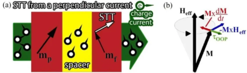
In 1996, Slonczewski [19] and Berger [20] independently predicted that a current flowing perpendicularly to the plane in a metallic multilayer could change the magnetization direction in one of the layers. In fact, when a current flows through a ferromagnet, all the electrons spins angular momenta become polarized along the same direction of the magnetization inside the ferromagnet: a polarized current is generated. This spin-polarized current can exert a spin-transfer torque (STT) on the magnetization of an adjacent ferromagnet, if it is not parallel to the first one (see Fig. 1.3). The mechanism responsible for the transfer of the spin-angular momentum is the exchange interaction “felt” by the electrons in the ferromagnet, which exerts a torque on the electron spins and, in turn, induces a reaction torque on the magnetization [21]. The possibility to manipulate the magnetization of a ferromagnet by means of a current, and not only of external magnetic fields, has opened new routes for promising applications of spin-transfer torque based devices, such as STT-Magnetic Random Access Memories (STT-MRAMs), spin-torque nano-oscillators (STNOs), nano-magnetic logic devices, etc. [22, 23, 24].

Fig. 1.3: schematic representation of the creation of the spin-polarized current. Part of the entering spins in the ferromagnet1 are polarized in the same direction of M₁, generating the spin-polarized current, which will transfer a spin-torque onto the magnetization M₂ of the adjacent ferromagnet2. Part of the entering spins is reflected with a polarization opposite to M₁.

12 Indeed, two types of STT can be considered: one acts when the current flows perpendicularly to the plane of a multilayer [19], and another one is exerted when the current flow is in-plane (IP) [20]. Basically, these torques arise in two different devices: the former in OOP devices, the latter in IP ones.

1.2.5 STT in OOP devices

Typical OOP devices are multilayered structures, made by two ferromagnets separated by a non-magnetic material. Usually, one of the two ferromagnet is thicker, in order to keep fixed its magnetization, and it is called pinned or fixed or reference layer or polarizer as well. The other ferromagnet is thinner to allow changes of its magnetization and it is called

free layer [21]. The chemical nature of the spacer leads to distinguish two

types of devices: if the spacer is an electrical conductor, the multilayer is called spin-valve; on the other hand, the presence of an electrical insulator spacer characterizes a magnetic tunnel junction (MTJ). When the electrical current density j_FE-oop flows perpendicularly to the device plane, it is polarized by the magnetization m_p of the pinned layer and, subsequently it will manipulate the magnetization mf of the free layer, via the STT τoop

(see Fig. 1.4(a)), which can be modeled as an additional contribution to the LLG equation, as derived by Slonczewski [19]:











being t the thickness of the free layer and (m m_f, _p) the polarization function, whose expression depends on the relative orientation between the pinned and free layer magnetization, the category of the device (i.e. spin valves, MTJs), thicknesses and ferromagnetic materials under investigation. In particular, for spin-valves the following ( m mf, p)expression is usually used [19]:

13









where  is the spin polarization factor related to the magnetic material. In the case of MTJs, the expression becomes [25]:





It is important to notice now that the Slonczewski torque acts as an anti-damping torque (or also “negative” damping) [26]. In fact, by comparing the damping torque in Eq. (1.28) and (1.30) with the STT expression in Eq. (1.31), it is possible to observe that they have a similar vector structure. Therefore, for a proper direction of the electrical current (more in detail, for positive current, which conventionally means electrons flowing from the free layer to the pinned layer), the two torques are opposite, implying that, while the damping torque tries to align mf with

p

m , the STT tries to avoid such alignment, pushing m_f away from m (see _p

Fig. 1.4(b)). The balance between these two torques is necessary to generate persistent oscillations of the magnetization in dissipative media [23, 26].

The dimensionless Landau-Lifshitz-Gilbert-Slonczewski (LLGS)

equation for a spin valve finally reads:









where the dimensionless time step d  ₀M dt_S has been introduced. Similarly, the LLGS for an MTJ is obtained:

14





















where, the main difference with Eq. (1.34) is the presence of an additional component of the STT term, namely the “field-like torque” or “out-of-plane” torque q V( )





MTJ leads [27].

Fig. 1.4: (a) schematic illustration of the spin-transfer torque exerted on the free layer magnetization in an OOP device. (b) representation of all the torques acting on the magnetization.

1.2.6 STT in IP devices

An IP device can be envisaged as a ferromagnetic strip with the length much larger than its width, containing magnetic regions with different internal magnetization (domains) separated by DWs. A current density j_FE-ip, flowing through the strip, is naturally polarized and can induce a translational motion of DWs. More specifically, when an electron flows in a ferromagnetic wire containing a single DW (see Fig. 1.5), the direction of its spin will adiabatically change, meaning that the electron spin will be almost parallel to the local magnetization. Such change in the spin direction gives rise to a STT which shifts the DW along the strip length. The expression of the adiabatic STT a

IP

τ was formulated by Berger [20] and reads:

15





being P the spin polarization factor, which represents the amount of spins polarized by the local magnetization.

Fig. 1.5: schematic representation of two domains (UP and DOWN) separated by a domain wall. A non-polarized electron flowing through this magnetization configuration will change the direction of its spin adiabatically, namely it will follow the local magnetization orientation.

Later, a second STT was phenomenologically added in order to explain unexpected early stage experimental results. It was called

non-adiabatic STT and its expression is:





where  is the non-adiabatic parameter. A complete description and physical origin of the two mentioned torques can be found in [28].

By considering the adiabatic and non-adiabatic STT, the dimensionless LLG equation for IP devices is:













1.2.7 Voltage controlled magnetocrystalline anisotropy (VCMA)

The application of an electric field can induce variations of the magnetic anisotropy of a ferromagnet, and, hence of its magnetization [29, 30]. The ferromagnet has to be ultrathin for at least two reasons: (i) its