A data-driven approach for early stopping in autonomous robot exploration based on convolutional neural networks

(1)

POLITECNICO DI MILANO

Scuola di Ingegneria Industriale e dell'Informazione

Corso di Laurea Magistrale in Computer Science and Engineering

A data-driven approach for early stopping

in autonomous robot exploration based on convolutional neural networks

Advisor: Prof. Francesco AMIGONI

Co-advisor: Dr. Matteo LUPERTO

Master thesis of:

LI Mingju Matr. 10574864/898045

LIN Chang Matr. 10597034/894651

(2)

(3)

LI Mingju / LIN Chang: A data-driven approach for early stopping in autonomous robot exploration based on convolutional neural networks | Master thesis in Computer

Science and Engineering, Politecnico di Milano. c

Copyright October 2019.

Politecnico di Milano: www.polimi.it

Scuola di Ingegneria Industriale e dell’Informazione: www.ingindinf.polimi.it

(4)

(5)

Acknowledgements

This thesis is finished with the help of many people. First we would like to thank our project supervisor, Prof.Francesco Amigoni, for giving us this opportunity to work on this thesis project, and our project advisor, Dr. Matteo Luperto for his continuous guidance, support and motivation throughout the project.

We would also thank our families and our friends. They provided us a lot of support and encouragement throughout our academic career.

(6)

(7)

Sommario

In questo lavoro di tesi, consideriamo le attività di esplorazione eseguite da robot mobili autonomi in ambienti interni. Durante l’esplorazione, il robot opera una sequenza di decisioni su dove andare e su quando fermarsi. In questa tesi, presentiamo un approccio di deep learning che permette al robot se fermarsi. Il nostro modello è stato sviluppato per terminare l’esplorazione quando le informazioni raccolte nella mappa sono sufficienti per ricostruire una mappa accurata, invece di terminare l’esplorazione quando ogni area dell’ambiente è stata effettivamente osservata. Le attività sperimentali, condotte in diversi ambienti in simulazione, mostrano che il nostro approccio è in grado di terminare l’esplorazione in modo tempestivo e di risparmiare una notevole quantità di tempo.

Parole chiave: AlexNet, ROS Simulation, Exploration Early Stopping, CNN,

Deep Learning

(8)

(9)

Abstract

We consider exploration tasks performed by an autonomous robot in indoor environments. During the exploration, the robot goes through a sequence of decisions on where to go and whether to stop. In this thesis, we present a deep learning approach that could decide whether to stop. Our deep learning model is developed to terminate the exploration when the map information is enough to reconstruct and output an accurate map, instead of terminating the exploration when every area of the environment has been actually observed. Experimental activities, performed in several different environments, show that our approach is able to terminate the exploration timely, and to save a significant amount of time.

Keywords: AlexNet, ROS Simulation, Exploration Early Stopping, CNN, Deep

Learning

(10)

(11)

List of Figures

2.1 This is an example of frontiers in a partially observed map. The

lines in different colors are all frontiers. . . 4

2.2 Here we show an example of the procedure of layout reconstruction [11]. . . 6

2.3 This is a very simple structure of a convolutional neural network [2]. 10 3.1 An example when the robot failed to stop timely. . . 18

3.2 The workflow of robot exploration with a baseline stopping criterion. 19 3.3 The observed map in relative early stage . . . 21

3.4 One scenario when the criterion "stop when the update of the map is small" does not fit . . . 22

3.5 The relationship of the exploration time and map coverage percentage [11] . . . 24

3.6 Observed map, compared with the ground truth map . . . 24

3.7 Reconstructed map, compared with the ground truth map . . . 25

3.8 The updated workflow . . . 27

3.9 The simplified model or our target early stopping module . . . 28

3.10 The goal of our current module to implement. . . 32

3.11 The structure of a common CNN network. . . 33

3.12 The structure of a CNN network with complemented information. 33 4.1 The current structure of AlexNet [19] . . . 40

4.2 The structure of a CNN with/witout dropout [42] . . . 40

4.3 Structures of our AlexNet. . . 44

5.1 The topics and nodes in our current ROS project) . . . 50

5.2 The communications between the navigator nodes and stopping criterion) . . . 51

5.3 The map distortion between the replayed map and ground truth . 56 5.4 An example of crop and resize . . . 58

5.5 An example of image feature augmentation . . . 59

5.6 The BC/FC output of 100 maps . . . 59

(16)

xvi LIST OF FIGURES

5.7 The visualization of data (blue are the maps that needs exploration,

and red are the well observed maps) . . . 61

5.8 Another kinds of visualization of data (blue are the maps that needs exploration, and red are the well observed maps) . . . 62

5.9 Two well observed maps . . . 63

5.10 Fuzzy function of map area . . . 65

5.14 Decision trees obtained from different attributes . . . 69

5.15 AUC ROC Curve [28] . . . 73

5.16 Visualization of underfitting and overfitting [36] . . . 74

5.17 The learning curve of cnn model of the optimal configuration . . . 76

6.1 An example of early stopping in test set . . . 81

6.2 Reconstructed layout of partial map of environment 2. . . 82

6.3 Environments in which early stopping perform badly. . . 83

(17)

List of Tables

3.1 Analysis on factor exploration time, exploration area. . . 29

3.2 Analysis on factor exploration time, exploration area. . . 30

3.3 Analysis on factor of current frontier numbers, frontier sizes . . . . 30

3.4 Analysis on factor of frontier shape . . . 31

3.5 Analysis on factor of observed map shapes . . . 31

4.1 Analysis on static rules model . . . 36

4.2 Analysis on map encoding model . . . 37

4.3 Analysis on deep learning (CNN) model . . . 38

4.4 Parameters of classical AlexNet structure . . . 39

4.5 Parameter and details of our AlexNet (Part 1) . . . 42

4.6 Parameter and details of our AlexNet (Part 2) . . . 43

4.7 Differences between our binary classfication task and previous general image classification task of AlexNet . . . 43

5.1 The responsibility during the project . . . 48

5.2 The topic information of /analyzer and /analyzerResult . . . 52

5.3 ROS bag info of one run in environment 7A-2 . . . 55

5.4 Two well observed maps and their BC/FC values . . . 63

5.5 Performance of cnn model in different configurations . . . 75

5.6 Confusion matrix of the optimal model . . . 76

6.1 The performance of our model in validation set . . . 80

6.2 The performance of our model in test set . . . 81

6.3 The performance of our model in online test . . . 85

(18)

(19)

Chapter 1 Introduction

Exploration by means of autonomous mobile robot is a task that incrementally builds maps of initially unknown, or partially known, environments [38]. At each stage of exploration, the robot decides whether to terminate the exploration process by using some criterion, and if not, decides the next location (often on a frontier between known and unknown space in the current map) to move to according to an exploration strategy [13]. When the selected location is reached by the robot, the map is updated according to the new knowledge of the environment and the process would re-start.

In this paper, we concentrate on the exploration of indoor environments. In previous work [11], the robot terminates the exploration when it has fully observed all the environment. We present a method to terminate the exploration process earlier, which could decide whether the current map is good enough to stop the exploration task because the unobserved parts can be reliably predicted.

To be more specific, we consider a mobile robot exploring an initially unknown indoor environment in order to build its 2D grid map. At each stage of the exploration, the layout of the known part of the environment could be extracted from the current partial map and the layout of the unknown part of the environment could be predicted by the method of [24]. The layout is an abstract geometrical representation of the rooms features and shapes [22]. The shape of partially observed rooms is predicted considering that different parts of the building share some common features. Different rooms could be related by the fact that they share the same shapes, and could be symmetric with each other.

The main original contribution of this thesis is that we came up with a method, which is data-driven, that could terminate the exploration process earlier with respect to cover all area until no frontiers left to explored. The stopping criterion in [11] could be regarded as a baseline stopping criterion. This baseline stopping criterion is relatively conservative in the terminating exploration. So, our early

(20)

2 Introduction

stopping criterion is developed to terminate the exploration earlier, and output a map, with a cost of potentially losing some accuracy. Experimental activities show that our approach is able to halve the time spent in the exploration in many different environments. Though there are some environments in which our model could not terminate the exploration early, this problem could be fixed by adding more environments in the training set.

The thesis is organized as follows. In the next chapter we will discuss the state of the art in robot exploration. In Chapter 3, we will formulate the problem we address in the thesis. In Chapter 4, several solutions will be proposed to solve the problem formulated, and in Chapter 5, details of implementation will be given. Chapter 6 includes the online and offine tests. At last, in Chapter 7, the conclusion will be made and future works will be discussed.

(21)

Chapter 2 Start of the Art

In this chapter, we would like to introduce the background knowledge and state of art technology related to our research. We are presenting an overview of other approaches that have been proposed in the literature for our problem, plus a set of techniques and methods that are relevant to the task of solving the problem of autonomous exploration of indoor environments.

2.1 Exploration

2.1.1 Definition

Exploration is the process in which an autonomous robot incrementally explores an initially unknown area [38]. The robot uses multiple sensors, including laser range sensor, collision detection sensors, to discover information of the current exploring map and use these information to make the decision of the next position to move. We assume that the robot has no prior knowledge of the map and all the information relative to the environment should be extracted from current observed map.

There are two main families of approaches which are mainly used in robot exploration.

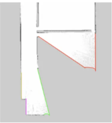
The first one is frontier-based approach. The frontier is defined as the boundary between known and unknown portion of the environment, as shown in Figure2.1. In this approach, the robot selects the next target location, which is a frontier, from the group of boundaries between known and unknown portions of environments [45].

The second is information-based, which moves the robot to the most informative locations. We select frontier-based approach since it naturally address the discovery of space for the problem of map building we consider [34].

(22)

4 Background

Figure 2.1: This is an example of frontiers in a partially observed map. The lines in

different colors are all frontiers.

Typically, at each stage of the exploration process, a robot selects the next best location according to an exploration strategy [13]. There are multiple exploration strategies which are commonly adopted in robot exploration. Usually most of these strategies are greedy due to the inherent online nature of exploration problem [39]. In a greedy strategy, the robot always selects the best solution of the current stage. Strategies can be defined by a single criterion or by combined criteria, to guide the next action of the robot. For example, a robot can always select the closest frontier for the reason of cost reduction, or select the frontier which is widest among the set of frontiers, since the widest frontier has intuitively the highest value for exploration. A better approach is to consider multiple criteria together, instead of a single one. For instance, [13] chooses the next frontier by both considering the distance from the robot current position and the expected information gain. This is also the approach adopted by our method.

2.1.2 Exploration Procedure

In our work, an exploration process [11] can be defined as following. A single robot is equipped with a laser range scanner with given field of view and range, which is able to build the map ME from the environment E. The map is not guaranteed to be the same as the environment, due to noise and error of the laser scanner. The robot starts to explore an initially unknown environment by frontier-based approach following the process below:

1. The robot observes a portion of E from its current position using its laser range scanner. Then it updates its partial observed map by integrating this portion.

(23)

2.2. Layout Reconstruction 5

3. According to an exploration strategy, the robot selects the next best frontier candidate.

4. The robot moves to the selected frontier and start from the first step again. The robot will repeat above steps until there is no frontier left. At this point, map ME _{could represents all free space of E.}

2.1.3 Information Gain And Distance

In order to apply a combined criteria for selecting the next best candidate, a common approach as [13] and [3] is to define an utility function. This function, given a frontier as input, outputs its utility value which represents how much it is worth if the frontier is selected as the best next one. The authors consider two criterias as a combined one. The first one is the distance utility, while the second one is the information gain of the frontier. The equation is shown below:

u(p) = α ∗ d(p) + (1 − α) ∗ i(p) (2.1) In the above equation, d(p) is the distance utility which is calculated as:

d(p) = (Dmax− D(p, pr))/Dmax (2.2) where D(p, pr) is the distance between the robot and the center of the frontier, and Dmax represents the maximum value of distance of all frontiers in the candidate set. i(p) is the information gain utility value, which is calculated as:

i(p) = I(p)/Imax (2.3)

where I(p) is the estimated unexplored area of the frontier, which can be obtained in the process of layout reconstruction (proposed in Section 2.2) and Imax is the maximum value of I(p) for all frontiers in the candidate set.

To combine these two criteria, a weighted sum needs to be computed, to represent the best balance between closeness and expected new area. By setting α to 1, the strategy becomes a closest-frontier strategy. As well, by setting α to 0, the strategy focuses only on expected information gain. Values of α can be selected by doing multiple test experiments.

2.2 Layout Reconstruction

To reconstruct the layout L of the environment starting from its partial map M , we use the method presented in [23] and [24]. We provide here a brief summary

(24)

6 Background

Figure 2.2: Here we show an example of the procedure of layout reconstruction [11].

of the algorithms using a running example as shown in Figure2.2. Please refer to the original papers for full details.

The algorithm starts from a grid map M of the environment, like the one in Figure2.2(a). A grid map is a map composed of a matrix of grids, in which each value represents the probability of the grid being occupied. From M a set of edges can be extracted, which are used to identify walls. Each wall is associated to a representative line by clustering. The representative line identifies the direction of the associated aligned walls. It means that all walls associated with the same representative line, even if they are in different portions of the environment, have the same direction. Representative lines can define a segmentation of the environment. Examples of representative lines can be seen, in red, in Figure 2.2(b). By this definition, after clustering all walls to a set of representative lines, a set of faces can be obtained by the intersection of representative lines (exactly four representative lines if the environment is rectilinear).

A face is the smallest unit representing potentially a room or part of a room, and a face could be one of the following three types:

• Fully observed, which means the area has been completely observed in M . • Partial observed, which means the area has been partially observed in M . • Unknown, if no point of the area has been observed in M .

After this step, we cluster all faces into clusters of faces, in which each represents a room. There are two different types of rooms:

• Fully observed room. This kind of room is composed of fully observed faces. • Partially observed room. This kind of room is composed of both fully observed

faces and partially observed faces.

Starting from fully observed rooms, in order to obtain a representation of the rooms, we follow the rules that fully observed room consists only of fully observed

(25)

2.2. Layout Reconstruction 7

faces and between any two faces there should not be any wall in M [26]. By traversing the whole set of fully observed faces and merging them, we are able to obtain a set of fully observed rooms. An example of fully observed rooms identified from the partial grid map of Figure2.2(a) is in Figure 2.2(c).

Afterwards, the best combination of fully and partially observed faces could be obtained, to generate the set of partially observed rooms by means of representative lines. The idea is to utilize some common structures or symmetries in floor plan layout architecture. We assume that the unknown environments we explore all share some common regularities. For example, if one side of the room is bounded by a corridor, then the other side of the room has a high probability to share the same wall with the neighbor room along the same corridor.

Practically, we usually start from the partially observed faces F , which contains at least a frontier. We iteratively consider all adjacent faces, including fully observed, partially observed, and unknown faces). Starting from F , we will also consider all adjacent faces of those faces and so on, up to a maximum number of hops from F (2 hops in our experiments). Afterwards, we generate a set of combinations of faces (they must be connected), of which each one could be a potential room. For each combination of faces F0, we try to calculate a utility value representing the probability of being an actual room. Here we introduce three criterias forming our objective function ϕ(F ∪ F0).

The first criteria is an intuition that the partial observed room (which is the combination of faces F ∪ F0) should have similar shape with respect to the rooms which are fully observed. To be more detailed, a combination would be better if an outer edge of the faces in this combination is longer and aligned to the representative lines. The second criteria follows the fact that commonly a room in a floor plan architecture usually has a simple shape (for example, rectangular) but not a complex shape (for example, concave polygon) and not a complex shape (for example, concave polygon). By means of this, we can compare the polygon formed by the combination of faces F ∪ F0 with that of its convex hull. The third criteria prefers the shapes which are delimited by a smaller number of walls.

Finally, the set of faces F ∪ F0{∗} that maximizes F ∪ F0 _{is then associated to}

the partially observed room. Then in this case, the polygon representing the layout reconstruction of rooms is obtained by merging faces F ∪ F0{∗}. As a result, we obtain a layout L = r1, r2, .. reconstructed which is completely composed of fully

(26)

8 Background

2.3 Backward Coverage And Forward Coverage

After the process of reconstruction, a correct layout should have the following two characteristics:

• All rooms in the ground truth (the actual layout of the environment) should be in the layout.

• All rooms in the layout should also be in the ground truth.

• The shape of each reconstructed room should be the same as that of the corresponding room in the ground truth.

Following the approach of [23] and [4], we introduce two measurements to compare the reconstructed layout L and ground truth Gt visually and numerically.

We introduce two mapping function between rooms of L and Gt, which are forward accuracy and backward accuracy. Forward accuracy represents how well the reconstructed layout is described by ground truth, while backward accuracy represents how well ground truth is described by the reconstructed layout. The mapping relationship can be shown as:

F C : r ∈ L 7→ r0 ∈ Gt BC : r 0

∈ Gt7→ r ∈ L (2.4)

For each room r ∈ L, forward coverage finds the room r0 ∈ Gt which has the maximum overlap area with r. As for backward coverage, for each room r0 ∈ Gt, it finds the room r ∈ L having maximum overlap area with r0. These two mapping functions can be used to calculate two accuray measurements, which are called forward accuracy (AF C) and backward accuracy (ABC). These two values can be calculated by the following equations:

AF C = P r∈Larea(r ∩ F C(r)) P r∈Larea(r) ABC = P r0∈Gtarea(BC(r 0 ) ∩ r0) P r0∈Gtarea(r 0 ) (2.5)

where area() is the function for calculating the area of a polygon, and the overlap between room r ∈ L and room r0 ∈ L is defined as area (r ∩ r0).

This accuracy measurement is able to measure the similarity between two layouts, especially between the reconstructed layout from the partially observed map and ground truth, due to the fact that a room is the best unit to describe and construct a floor plan layout in our problem.

At the early stage of exploration, the partial map only covers part of the ground truth, with a relatively high AF C and a relatively low ABC. That’s because for a room r (fully or partially observed) in the layout built from the partial map, we are always able to find the real room r0 in ground truth which almost (due to noise

(27)

2.4. Convolutional Neural Network 9

and error) completely covers the area of room r. And this room apparently has the maximum overlap area. On the contrary, for a room r0 in ground truth which is still unexplored in the partial map, it’s apparently impossible for find a overlap room r in the partial map. That’s the reason why we will obtain a high AF C and low ABC.

When the partial map is almost fully explored, we will obtain a high AF C and high ABC if the method correctly reconstructs the layout from the partial map.

2.4 Convolutional Neural Network

Nowadays, with the devolpment of machine learning and deep learning, convolu-tional neural networks are commonly used in many domains, both scientifically and industrially. Image classification and object recognition are two of these domains, while autonomous exploration is considered in this thesis. In this section, we will first describe the basic theory of convolutional neural networks, then propose they can be used in some application domains, especially autonomous exploration of unknown environments.

2.4.1 Introduction

Convolutional neural networks (CNNs) are a type of feedforward neural net-work with convolutional computation and deep structure. It is one of the most representative algorithms of deep learning [17] [15]. Convolutional neural networks have the ability of representation learning, which means instead of learning pre-designed features, CNNs could discover features and learn these features, and are able to shift-invariant classify the input information according to their hierarchical structure. Therefore, it is also called “Shift-Invariant Artificial”.

The study of convolutional neural networks began in 1980s and 1990s. The time-delay network and LeNet-5 were the earliest convolutional neural networks [21]. After the 21st century, with the introduction of deep learning theory and the improvement of numerical computing device, convolutional neural network has been rapidly developed and applied to computer vision, natural language processing and many other fields.

The convolutional neural networks can perform both supervised learning and unsupervised learning. The kernel parameter sharing in hidden layers and the sparseness of the inter-layer connection guarantee that convolutional neural network is able to extract features from grid-like topology in a small computational cost. Therefore, convolutional neural network can learn from pixels or audio with a stable effect and have no additional requirements for feature engineering [17] [15].

(28)

10 Background

2.4.2 Theory Support

Basic Structure

A convolutional neural network consists of multiple convolutional layers and one or more fully connected layers at the top (corresponding to a classical neural network), and also includes associated weights and pooling layers. This structure enables the convolutional neural to take advantage of the two-dimensional structure of the input data. By this feature, convolutional neural network gives better results on image and speech recognition than other deep learning structures. Figure 2.3 shows a standard convolutional neural network structure:

Figure 2.3: This is a very simple structure of a convolutional neural network [2].

Input Layer

The input layer of a convolutional neural network can process multi-dimensional data. Commonly, the input layer of a one-dimensional convolutional neural network receives a one or two-dimensional array, in which a one-dimensional array is usually sampled by time or spectrum, while a two-dimensional array may contain multiple channels. A two-dimensional convolutional neural network receives a two or three-dimensional array, and so on [29]. Since convolutional neural networks are widely used in the field of computer vision, many studies presuppose three-dimensional input data, which are the width, length and the color channels of the pictures.

(29)

Similar to other neural network algorithms, the input features of the convolu-tional neural network need to be normalized since we use gradient descent as the learning algorithm. Specifically, before we input the data into our convolutional neural network, we need to normalize the input data in the dimension of channel, time, or frequency. For example in computer vision, the original pixel values could be normalized to a specific interval. By normalization, we are able to improve the learning efficiency and performance of our convolutional network [29].

Convolutional Layer

The hidden layer of the convolutional neural network includes three common constructions, which are convolutional layer, pooling layer, and fully connected layer.

The function of the convolutional layer is to perform feature extraction on the input data, and contains multiple convolutional kernels. Each element in the convolutional kernel corresponds to a weight coefficient and a bias vector, similar to the neuron in feedforward neural network. Each neuron in the convolutional layer is connected to a plurality of neurons in a region of the previous layer. The size of the region depends on the size of the convolutional kernel and is called “receptive field” in the literature [15]. Its meaning can be analogous to the receptive field of visual cortical cells in animals. When the convolution kernel is working, it will regularly scan the input features, multiply the input features by matrix elements in the receptive field, and add the bias [17]:

Zl+1(i, j) = [Zl⊗ wl_{](i, j) + b =} Kl X k=1 f X x=1 f X y=1 Z_kl(s0i + x, s0j + y)wl+1k (x, y)] + b (i, j) ∈ {0, 1, ..., Ll+1} Ll+1= Ll+ 2p − f s0 + 1 (2.6) The above equation describes how convolutional kernel works in each convo-lutional layer. The summation in the equation is equivalent to solving a cross-correlation. b is the bias. Zl _{and Z}l+1 _{represents the input and output of the (l+1)} convolutional layer, which is also known as the feature map. Ll+1 is size of Zl+1 since here we assume that the width and the height of the feature map are the same. Z(i, j) corresponds to each pixel in the feature map. K is the number of channels of the feature map. f , s0, and p are the parameters of convolutional layer,

corre-sponding to convolutional kernel size, convolution step (stride), and padding. These three values are hyperparameters of the convolutional neural network, together determining the size of the output feature map of convolutional layer [17].

(30)

12 Background

Kernel size can be specified as any value smaller than the input image size. The larger the convolutional kernel, the more complex the input features extracted from the input image. The convolution step (stride) defines how many pixels the convolutional kernel shifts at each step. In other words, stride controls how the filter convolves around the input volume. For example, when stride is set to 1, the convolutional kernel sweeps the elements of the feature map one by one. If set to n, the convolutional kernel skips (n − 1) pixels and shifts to the nth one [9].

As it can be known from the cross-correlation calculation of the convolutional kernel, the size of feature map will gradually decrease with the stacking of the convolutional layers. For example, consider a 16 × 16 input image. After convolved by a 5 × 5 convolutional kernel with one stride at each step and no padding, a 12 × 12 feature map is output. Padding is a method of increasing the size of a feature map before is passes through the convolutional kernel to offset the effect of dimensional shrinkage in the calculation. A common padding is padding with zero and repetition padding by boundary value.

The convolutional layer also contains the activation function which helps to express complex feature, represented as following [17]:

Al_i,j,k = f (Z_i,j,kl ) (2.7)

where Z_i,j,kl is the output of each convolutional layer and Al_i,j,k represents the value after activation.

Like other deep learning algorithm, convolutional neural network usually uses Rectified Linear Unit (ReLU) as activation function. Some other variants like ReLU includes Leaky ReLU (LReLU), parametric ReLU (PReLU), randomized ReLU (RReLU), and so on [15]. Activation function is commonly used after the convolutional kernel, while some algorithms using preactivation techniques place the activation function before the convolution kernel.

Pooling Layer

After feature extraction in the convolutional layer, the output feature map is passed to the pooling layer for feature selection and information filtering. The pooling layer contains a predefined pooling function, which replaces the result of previous convolutional layers. The way pooling layer selects pooling area is similar to convolutional kernel, controlled by the pool size, step size (stride), and padding [17].

(31)

Fully Connected Layer

The fully connected layer in a convolutional neural network is equivalent to the hidden layer in a traditional feedforward neural network. The fully connected layer is usually build at the last part of the hidden layers in convolutional neural network, and only passes signals to other fully connected layers. The feature map looses the three-dimensional structure in the fully connected layer, and is expanded into a vector and passed to the next layer through the activation function.

In some convolutional neural networks, the function of fully connected layer can be partially replaced by global average pooling [35]. The global average pooling will average all the values of each channel in the feature map. For example, considering a 7 × 7 × 256 feature map, the global average pooling will return a 256 vector, where each element is a 7 × 7 average pooling with stride equals to 7 and no padding.

Output Layer

The upstream of the output layer in the convolutional neural network is usually a fully connected layer, so its structure and working principle are the same as those in the traditional feedforward neural network. For image classification problems, the output layer uses a logic function or a normalized exponential function (softmax function) to output the classification label. In object detection problems, the output can be designed as the center coordinate, size, and classification of the output object. In semantic image segmentation, the output layer directly outputs the classification result for each pixel [29].

2.4.3 Applications

Image Classification

For a long time, convolutional neural network has been one of the core algorithms in the field of image recognition, and has a stable performance when learning a large amount of data [10]. For general large-scale image classification problems, convolutional neural network can be used to construct hierarchical classifiers [33]. It can also be used in fine-grained recognition to extract discriminant features of images for other classifiers to learn [40]. For the latter, features can be extracted artificially from different parts of the image [5], or by the convolutional neural network through unsupervised learning [18].

For text detection and text recognition, a convolutional neural network is used to determine whether an input image contains characters and to clip valid character segments from the image [46]. For example, the convolutional neural network

(32)

14 Background

using multiple normalized exponential functions is used for the identification of the numbers in Google Street View Image [14]. Also in recent research, a convolutional neural network combined with a recurrent neural network (CNN-RNN) can extract character features and process sequence labelling [16].

Object Recognition

Convolutional neural network can be used for object recognition through three types of method : sliding window, selective search, and YOLO (You Only Look Once) [15]. The sliding window was used for gesture recognition [30]. But, due to the large amount of calculation, it has been eliminated by the latter two. Selective search corresponds to region-based convolutional neural network. It first determines whether a window may contain a target object through general steps, and further inputs into a complex identifier [12]. The YOLO algorithm defines object recognition as a regression problem for the probability of occurrence of each target in a segmentation box in the image, and uses the same convolutional neural network to output the probability, the center coordinates, and the size of the frame [32]. Object recognition based on convolutional neural networks has been applied to autonomous driving [25] and real-time traffic monitoring systems [20].

Autonomous Exploration

Convolutional neural networks can also used in the field of autonomous explo-ration of unknown environments. In recent research, [8] proposed the application of convolution neural networks in predicting human trajectory in environment. The authors use the model to predict average occupancy maps of walking humans even in environments where no human trajectory data are available. With such a predictive model, a robot can use this information to find nondisturbing waiting positions, avoid crowded areas, or clean heavily frequented areas more often. This approach transfers from simulation to real world data, and generalizes better to new maps than five baselines and surpasses the performance of the baseline models even when they are applied directly to the test set.

[6] proposed another application of convolutional neural networks in autonomous exploration of unknown environments by predicting future observations. The author trains a convolutional model using a database of building blueprints, which exploits the inherent structure of buildings. The model guides the robot to find the exit location of buildings. Comparing to traditional image processing apporaches of extracting features through histogram of gradients (HOG) and training a support vector machine (SVM), this method reduces the total exploration time to find the exit location by 36%.

(33)

2.5. Summary 15

Both these two methods take advantage of the ability of feature extraction and abstraction of convolutional neural network acquired. In domains of autonomous exploration, most of the input images are maps obtained by the robot in a specific environment. Comparing to image classification and object recognition, these data are simpler (usually with only one channel), and the structure of lines and corners is much more obvious, which means the convolutional model is able to extract enough features for prediction even without a large amount of training data.

2.5 Summary

In this chapter, we presented an introduction of the state of the art of exploration and deep learning in autonomous exploration. First of all, we briefly introduced how exploration problem is defined and the general solution we used for solving an exploration problem. Secondly, we detailed the methods we used for reconstructing the layout of the partial map. Afterwards, we described an intuitive method to measure the quality of the reconstructed layout of a partial map. Finally, we illustrated what a convolutional neural network is and how the model could be used in multiple application fields, including autonomous exploration.

(34)

(35)

Chapter 3 Problem Formulation

Chapter 2 introduces the state of art methods in robot exploration, while in this chapter we will focus on early stopping criterion in the exploration process, and fomulate the problem we address in the thesis. The robot with layout reconstruction information gain exploration strategy introduced above could works stably in many cases. However, in many cases, we want the robot to be fast in exploration.

Faster exploration speed could help us build a map in a shorter time. Sometimes, like in search, the time spent on building a map could be more important than some single details of the map. Even in some domestic tasks, we want our robot to be fast, knowing the fact that sometimes this means it maybe reckless in a way.

3.1 Motivations

In this section, we would like to introduce the motivation of what problem we found in this process of exploration with more details and statistics.

Though in the previous part of thesis, "early stopping criterion" / "early stopping criteria" have been mentioned for several times, it is necessary to provide a formal definition of this terminology. Generally speaking, the exploration process consists of exploration and stopping condition, which will give an answer for the question, "whether the agent should be stopped". Stopping criterion notifies the robot whether the map has been fully explored and it should terminate the exploration process. Method in [11] implements the criterion that "stops when no effective frontier exists" as a stoppoing criterion. Early stopping criterion, based on stopping criterion, is a method to stop before it has detected every area in the environment, when it could provide a correct reconstructed map, based on its current exploration progress.

From the thesis of [11], the robot stops exploration when it has already observed the whole environment space. Consider the fact that in our exploration process, the robot always selects the frontier with the highest utility value2.1.3, and usually

(36)

18 Chapter 3. Problem Formulation

with a relatively high information gain 2.1.3. Therefore, the robot is able to quickly increment the knowledge of its map. However, it will also leave small scattered frontiers across different rooms, as a consequence of their small information gain. Then in the final stage of exploration (usually when the total area explored reaches 80%), the robot needs to reach all the remaining small frontiers.

The time cost for reaching all those frontiers is particularly high. They are usually located in rooms that are far away from each other, representing small gaps like corners, with a low information gain. Therefore, we can avoid the exploration in these small frontiers if we are able to introduce a mechanism for the early stopping of exploration.

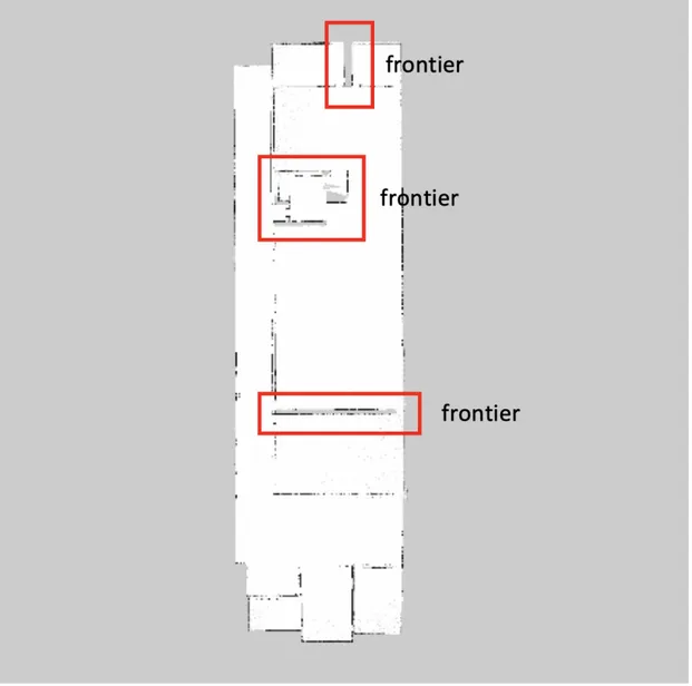
Figure 3.1: An example when the robot failed to stop timely.

Figure3.1shows the state of one partially explored map. It is not hard for us to conclude that this map is well explored, and we could stop and output a complete

(37)

3.1. Motivations 19

map. Nevertheless, our robot, with its current stopping criterion, detects some tiny frontiers, and regards those frontiers as potential next destinations.

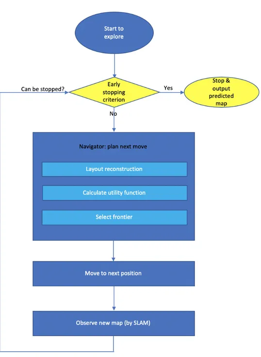
3.1.1 Current Early Stopping Criterion

In current exploration strategy, a baseline stopping criterion, that "stops when no frontier exists", has been implemented in the system. Figure3.2 represents the workflow and relationships between different modules in our exploration.

(38)

Popular baseline stopping criteria include the following techniques. * Stop when there is no frontiers in the map

In every moment in the grid map, as shown in Figure3.3, three kinds of pixels could be observed, free space, obstacle, unknown space. We call the set of continuous pixel between free space and unknown space "frontier". And here in this stopping criterion, we only stop when there is no frontier left in the diagram. First, we have to filter noise, which is represented by tiny frontiers. After filtering, we analysis whether there is any effective frontier left, which could lead the agent to a new room or space. If the answer is positive, keep on exploring, else, stop exploring.

This is a popular and basic stopping criterion applied in todays applications due to the reason that it is easy to be implemented. It is robust, because actually how it works is that "it never gives up any oppotunities". However, this also lead to the problem that the exploration process always takes longer than needed.

* Stop when the update of the map is small

If an effective exploration is being executed, the map should be updated continuously, and we expect our map covers increasingly more area. Hence we could use this property to stop the exploration. Assuming map area at time stamp t1 is M apt1_{, and our map area at time stamp t2 is M ap}t2_{. The} area increase between two timestamps is

∆M ap = M apt1− M apt2

We could set a threshold for this ∆M ap. If the ∆M ap is zero for a long time, it is reasonable to believe the map is well explored and we could stop. Of course, more details are needed to make this method work. The most significant thing is that we must assure that our navigator module works normally. And another thing we must take into consideration is that it would take a relative long time for a robot, moving from one position to another position, especially when the structure of the building is very complex. During the moving process showed in Figure 3.4, the robot may detect no map area increase for a relative long time, but we still could expect that some new area could be found by our robot from the target position.

Compared with current stopping criterion, a new stopping criterion, "stop when the prediction area is small" could be introduced. This stopping method estimates

(39)

3.1. Motivations 21

(40)

Figure 3.4: One scenario when the criterion "stop when the update of the map is small"

(41)

3.2. Current Time-area Diagram And Analysis 23

the amount of unexplored area, and stops exploration when it’s lower than a predefined threshold. By using our layout reconstruction algorithm, we are able to predict the missing part of the partially observed rooms, and automatically fill these small gaps without actually explorating them. Therefore, we could introduce a criteria of early stopping based on the reconstructed layout. By the work of [24], if the unexplored area for all candidate frontiers could be predicted, and the total amount of such area is less than 1 m2 _{or of another threshold, exploration would be}

terminated. We can assume that the robot can finish the exploration process and discard all remaining frontiers since we are able to predict the area beyond them from the corresponding reconstructed layout.

However, this mechanism has its limitations which are hard to avoid in practical situations. The first limitation is that it’s hard to decide the threshold for early stopping, due to the fact that we have no prior knowledge about the unknown environment we explore. The environment could be large, like school or hotel. But it can also be just a combination of four rooms, being the house of a family. Therefore, no matter how we choose a static threshold, there will always be some cases which are out of the scope. The second limitation lies in the use of unexplored amount of area as a measurement. To decide whether the robot can stop exploration or not, using area as a single measurement is sometimes not enough. Therefore, as will be proposed in later chapters, we introduce a new data-driven method to predict the correct timestamp for early stopping, taking advantages of convolutional neural networks.

3.2 Current Time-area Diagram And Analysis

In this section, we perform some analysis and visualization on the data we obtained from using the stopping criterion in [11] (stop when no frontier exists). The information shown in Figure 3.5 is extracted from environment 41-1.

In Figure 3.5, we could see that the robot spends almost 50% time to cover the last 10% part of the map. Here we select the map at about 3600 seconds, and below are the diagram of observed map (at timestamp 3600 seconds) vs ground truth, and the diagram of predicted map vs ground truth.

On the left of Figure 3.6 is the observed map at 3600 seconds, on the right of Figure3.6 is the ground truth. We could see that at this timestamp, we have already covered most of the areas in the ground truth. Though it is possible that in the right bottom corner of the map still exists a corridor, or a door to another room or area, we can reliably predict the shape of the map, and stop the exploration process with some degree of confidence.

(42)

Figure 3.5: The relationship of the exploration time and map coverage percentage [11]

(43)

3.3. Problem Formulation 25

Figure 3.7: Reconstructed map, compared with the ground truth map

right of Figure3.7 is the ground truth. In our layout reconstruct method, we use different colors to represent different rooms. Here it could be seen that there is only one small corner missed in this prediction.

In the balance of time efficiency and map accuracy, we have to choose which one is prefered. Sometimes we could tolerate that, just like above situation, one small corner is missed, but sometimes we could not allow that, and we aim for our robot not to miss anything.

Of course the predicted map is not a 100% equal to the ground truth. Besides the small room on the right bottom corner, the big blue room on the right side of the predicted map is not accurate. This is because these colored rooms are obtained by the clustering algorithms. By adopting different values of parameters, we could get different clustering results. So this could not be regarded as a false prediction. However, still we need some good methods to combine the predicted map with the observed map to output a final map as result of exploration. But this would not be discussed in this thesis.

Being able to stop early is an important ability for the robot. Since it could send a signal to the user or administrator that they could trust the current map. We will start from this idea to find a solution for early stopping in exploration of indoor environments.

3.3 Problem Formulation

From the analysis above, it is quite easy to find that in our current exploration strategy, the autonomous agent keeps on exploring the environment even when it

(44)

could do some prediction based on the layout reconstruction method and output an accurate map compared with the ground truth.

If we could come up with a method that could effectively tell whether the robot could stop and do a prediction, some time could be saved. This could be a very great improvements in applications of autonomous exploring agents.

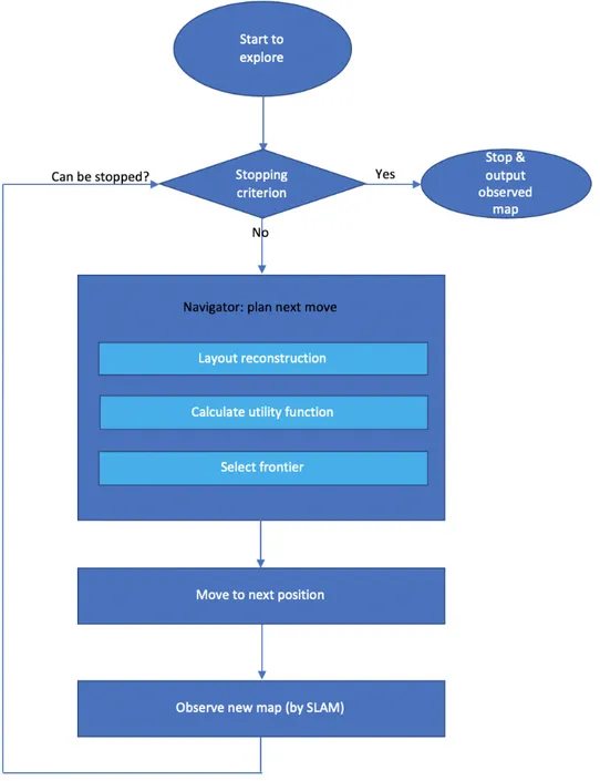
So now the problem could be formulated as building a model, given the in-formation of the map and exploration process, that could output a conclusion either “we could stop exploration, and output the reconstructed layout as the exploration result” or “further exploration is needed to generate an accurate map layout reconstruction” (just as the yellow modules in Figure 3.8).

To be more specific, as shown in Figure 3.9, the problem to be solved is how to predict “a given map is a well-observed map” is TRUE or FALSE. Here this “well-observed map” means a map that is almost completely explored, and for those areas we have not observed so far, our current layout reconstruction could provide a relative accurate prediction, and an accurate predicted map could be reconstructed and output.

The information we mentioned about the map and the exploration process includes but is not restricted to: the shape of the map, the scale of the map, the relationship between one single pixel and real area it represents in the environment, the exploration time. With this information, we could use some data driven methods to build a model to do a prediction.

3.3.1 Assumptions

First, we have to set some assumptions that could help us in our research. For most of the assumptions made here, they are not 100% accurate, but we could expect them to be correct in most cases. By doing so we could simplify our problem. These assumptions include:

1. The simulation with ROS[31] could simulate the real exploration process In this thesis, most of our analysis are based on the simulation result performed on ROS. Hence we should trust this ROS simulation process, the simulation process showed in our ROS system could represent the robot action in the live environments. This includes the computing ability of the agent in live environment should be better than what we simulate in ROS. And the execution of the planning trajectory, layout reconstruction, and SLAM in the real environment should be executed just like how it is done in ROS.

(45)

(46)

Figure 3.9: The simplified model or our target early stopping module

For simulation, we choose a 180 degree laser-sensor in ROS. However there are several cases we could expect during collecting sensor information. The first one is that solid obstacles could be detected in the sensor. However, in another situation, the sensor may detected nothing in its reception range. And in this cases, it would have a shape like a fan-shape area during simulation, and we assume this shape is same as the real environments.

3. We always consider indoor environments

In our research, we only considerindoor environments. Any other environment like forests and underground caves are not taken into consideration, because these natural architecture are very different from the artificial building. All of our training and testing data (100 environments) are obtained from the indoor buildings datasets.

4. The floor is clean

We always assume that the environment has a clean floor, or the robot could regard those obstacles as noise when dealing with them. For all the environments we are dealing with, they have the same elevation.

We could proposed several solution for this formulated problem in Table 3.1. The factors that could potentially help us decide the status of the map are listed with different granularities. Explanation is attached for each factors.

(47)

Granualrity Factor Name Explanation

Global Time Is there a time boundary that we could say a map is well-observed (after the exploration taking t seconds, we could conclude a map well-observed).

Map Map Shape Is there any image analysis technology we could apply on the map (given the map shape, do the prediction).

Map Map Area Is there any pattern on the area of the map (when the area of the map is greater than m m2_{, we could say that map is well observed).}

Frontier Frontier Number Is there any rule on the number of frontiers (when the number of frontiers is less than n,

we could conclude a map is well observed). Frontier Frontier Size Is there are any rule of the frontier size (if

the frontier is smaller than a threshold f s, we could say that no further exploration is needed on this map).

Frontier Frontier Shape Is there are any image analysis technology we could apply on the frontier shape (given a specific frontier shape, we could conclude this frontier no longer needs any further ex-ploration).

(48)

* Global: It means these factors are considered globally during the exploration process (exploration time, ...).

* Map: It means these factors are directly related to the maps (map area, map complexity, map shape, ...).

* Frontier: It means these factors are directly related to each frontier in the maps (frontier size, frontier numbers, frontier shape, ...).

Here we do some further analysis on these factors in Table3.2, Table 3.3, Table 3.4 and Table3.5.

Exploration Time, Map Area Covered

Pros Easy to measure.

Cons For different maps and robots, even different exploration speeds, the time spent on a single map could be really dif-ferent, it could hardly represent the progress of our current exploration. And for the map area it is the same as well. Conclusion We could use time and map area as a complement criterion in

the early stopping criterion. However, no direct relationship between these factors and exploration status is expected in real situation.

Table 3.2: Analysis on factor exploration time, exploration area.

Frontier Number, Frontier Size Pros Easy to do statistics and find the rules.

Cons The number of frontiers is not a very representative factor for the map, because in real situations (in most situations), there are not too many frontiers, but maybe there is just one frontier that leads to another new area and rooms.

Conclusion Could not be chosen as one of the main factors to decide.

Table 3.3: Analysis on factor of current frontier numbers, frontier sizes

To summarize above information, we could reach this conclusion. The early stopping criterion is closely related to many factors and information collected during the exploration process. However, from a practical point of view, the best direction to start from is to start from map shape analysis with data driven techniques.

We would like to further clarify our goal and solution with details in the next section.

(49)

Frontier Shape

Pros Enough data could be obtained, since for each map we could sample about three or four frontiers.

Cons The data is enough, but we have to decide what area should be cropped out, because for the frontier what is important is not their shape, but the shape of obstacles (those solid boundaries obtained by sensors) around them.

And another problem is that it is not easy to label these frontiers, for three or four frontiers we found in the map, only one of them could be the reason why the agent still needs to explore. So the labelling is not easy to be implemented, we need some exquisite method to do this labelling.

Conclusion This is a promising method we could explore.

Table 3.4: Analysis on factor of frontier shape

Map Shape

Pros The most direct and global information for the map status, could be very effectively labelled and checked.

Cons We hold just 100 environments, even if we have about 30 to 40 runs for each environments, 100 is a small number when it comes to learn general rules. Data enhancement methods should be applied. And new environments should be added to our current training set.

Conclusion This is the best direction we should go along.

(50)

3.4 Goal

With above analysis, our goal is to build a model to classify the statement “current map is well-observed” is true or false. The input of the model is the map

shape and the output is a binary classification of true or false.

We could abstract this problem into a binary classification task on images. And for these images, we know there are some special features, compared with common images:

* Single channel Our images are grayscale single channel images, could be represented by a 2D arrays.

* Simple values For the elements appearing in the 2D array, there are only 3 unique values, meaning free pixel, unknown pixel, obstacle pixel.

It would be a good idea to keep these properties even during processing input images, because these simple properties could help us to be more robust against the noise and information loss happening in data processing.

And besides the map shape, other information listed above could be added into the system as a complement for the model, as shown in Figure 3.10. Since they could be related to the map complexity and map scale, they are all good measurements for this kinds of abstract values.

Figure 3.10: The goal of our current module to implement.

Now to simplify the model we are dealing with, we just consider the model with one input, that is the map shape. While still it is possible to attach other information on this image input (input the model with a map shape of .png/.pgm format and another file recording all the context for the map with .xml/.yml formats). Another idea is that we could try to re-encode our map file with the

(51)

3.4. Goal 33

context information, like setting the color to be lighter if the map is big, and setting the color to be darker if the map is small. Last but not least, we could integrate these context value in our fully connected layer if we are dealing a convolutional neural network + fully connected layers deep learning models. Figure 3.11 is a common structure of a normal CNN+FCL model.

Figure 3.11: The structure of a common CNN network.

And we could integrate those complement information in the flatten input of fully connected layer, because before the fully connected layer, the result of the convolutional layer must by flattened to one array. Hence these complement information could be of help just as shown in Figure 3.12.

Figure 3.12: The structure of a CNN network with complemented information.

(52)

improve the model performance based on our current model performance, but this will not be discussed in our thesis.

3.4.1 Summary

In this section we would summarize all the points mentioned in this chapter. The problem we are dealing with is that we want to add an effective early stopping decision system into our current autonomous exploration agent. Hopefully it will inherit the advantages of the "stop when no frontier exists", which means it should be robust, and would not give false prediction when the map still needs exploration. But, at the same time, it could stop earlier.

This new model could decrease the time spent on those areas for which we could easily predict their shape, and speed up the whole exploration process.

The best way to realize such goal is to apply data-driven techniques, building a model, which could classify input map to be “well observed” or not.

(53)

Chapter 4 Proposed Solution

To reach the goal mentioned above, we have several ideas to realize the model. In this chapter, we will discuss all the possible solutions we offered, their advantages, and their disadvantages. And in the later part of this chapter, we will pick out one of the most practical methods (CNN), and gives more details about why we could use it to solve this problem, and how we could do that.

4.1 General Overview

To build a model which could solve the above problem, we have these ideas.

(54)

36 Chapter 4. Proposed Solution

* Static and manually designed rules in Table 4.1 Static and Manually Designed Rules

How We could go through all the map information we have trying to summarize the features, and design a set of rules. To do so, we could follow this procedure

* Use image analysis method to capture special features in the map (corners/frontiers/open areas).

* Do statistics on these features and the maps to find the relationships between them.

* Design a set of rules (if no fan shape appears in the image, assert true/elif the number of corners>n, assert false / ...).

Pros

* Readable, reasonable and understandable rules. * Could be modified and edited easily.

* Easy programming, and implemented with ROS system.

Cons

* Not easy to be designed, quite hard to find the potential rules.

* Hard to be implemented for the rooms with different scales.

* Hard to be implemented for the rooms with peculiar shapes.

Conclusion NOT suitable

(55)

4.1. General Overview 37

* Map Encoding techiniques in Table4.2

Map Encoding Techiniques

How The core idea of this method is to abstract the structure of the map, and then learn its structure. It could be done using following procedure.

* Abstract the map into an undirected graph. For each room, corridor, extract them into a node in the graph, for each door, connection, extract them into a undirected edge.

* (Manually) label these graphs.

* Learn and generate the possible patterns and rules for these graphs.

Pros

* Easy to visualize.

* Very light-weight model.

Cons

* Undirected graphs are hard to compare (could lead to a NP problem).

* No mature models to learn these kinds of structures and tasks.

Conclusion NOT suitable

(56)

* Deep learning models with image analysis method in Table 4.3

Deep Learning Techiniques

How We could build deep learning models with Convolutional Neu-ral Networks + Fully Connected Layers structures. To do so, we have to follow this procedure.

* Data extration and preprocessing. * (Manually) label training data. * Define loss function.

* Define CNN structure.

* Feed the data to our model and training. * Parameter fine tuning.

* Validation. * Offline test. * Online test.

Pros

* Mature method, a lot of previous research results and sucessful industrial applications could be found.

* Good performance in image (binary) classification task. * Easy to be implemented and integrated.

* Fit well in peculiar shape buildings. * Does not influensed by the building scale. * Robust to noise.

Cons

* Training takes time.

* Limited data (we only have 100 environments), and the result may be not representative enough.

Conclusion Suitable

(57)

4.2. AlexNet 39

4.2 AlexNet

In chapter 2, we have already introduced convolutional neural networks, and their applications in real world. In the area of advanced image classification, they are the best performance tools we have so far.

Nevertheless, convolutional neural networks are a great class of deep learning models. In the family of convolutional neural networks, GoogleNet, PReLUNet, Vggs and SqueezeNet are some of the most advanced CNN structures with the core idea of convolutional layer to extract features, and fully connected layer to execute the classifications. They have reach very high accuracy in the ImageNet image classification task. To achieve our goal, we select AlexNet to carry out this task.

4.2.1 AlexNet Defination, And History

AlexNet [19] is known as one of the most mature, famous, and influential convolutional networks. We could almost say that the victory of AlexNet on ImageNet in 2012 started the era of deep learning. Later advanced CNNs also inherit some parts of AlexNet characteristics.

The most well-known AlexNet has following parameters in Table 4.4: Number of convolutional layers 5

Number of fully connected layers 3

Depth 8

Number of parameters 60M

Number of neurons 650k

Number of classification 1000

Batch normalization None

Table 4.4: Parameters of classical AlexNet structure

The general structrues of AlexNet could be represented as Figure4.1.

As a epoch-making deep learning structure in 2012, AlexNet has these charac-teristics which helped it winning the ImageNet in 2012.

1. Data Augmentation

Horizontal flipping, random cropping, object shifting, color transformation, lighting transformation, contrast transformation, etc. These effectively added more data to the training set and could keep the model away from overfitting. 2. Dropout

(58)

Figure 4.1: The current structure of AlexNet [19]

In all kinds of deep learning methods, the overfitting is an inevitable problem we are going to face in the model training. Take AlexNet as an example, we have 60M of parameters. And for the training set, our data is relatively limited compared with such a huge system. So it is very important to solve this problem.

Dropout is one of the method applied by AlexNet. The core idea of dropout could be summarized in Figure 4.2: when we are trying to perform forward propagation, we make a neuron stop working with probability p. This could significantly enhance the generalization ability of our model, because it means that it will not strongly depend on some local characteristics.

Figure 4.2: The structure of a CNN with/witout dropout [42]

3. ReLu Activation Function

Activation function is designed to keep the non-linear properties of the net-work [27]. Before AlexNet, tanh activation function and sigmoid activation

A data-driven approach for early stopping in autonomous robot exploration based on convolutional neural networks

POLITECNICO DI MILANO

Scuola di Ingegneria Industriale e dell'Informazione

Corso di Laurea Magistrale in Computer Science and Engineering

A data-driven approach for early stopping

in autonomous robot exploration based on convolutional neural networks

Acknowledgements

Sommario

Abstract

Contents

List of Figures

List of Tables

Chapter 1

Introduction

Chapter 2

Start of the Art

2.1

Exploration

2.1.1

Definition

2.1.2

Exploration Procedure

2.1.3

Information Gain And Distance

2.2

Layout Reconstruction

2.3

Backward Coverage And Forward Coverage

2.4

Convolutional Neural Network

2.4.1

Introduction

2.4.2

Theory Support

2.4.3

Applications

2.5

Summary

Chapter 3

Problem Formulation

3.1

Motivations

3.1.1

Current Early Stopping Criterion

3.2

Current Time-area Diagram And Analysis

3.3

Problem Formulation

3.3.1

Assumptions

3.4

Goal

3.4.1

Summary

Chapter 4

Proposed Solution

4.1

General Overview

4.2

AlexNet

4.2.1

AlexNet Defination, And History