Fixed-term jobs, skills and labour market performance

(1)

UNIVERSITÀ' DELLA CALABRIA- FACOLTÀ' DI ECONOMIA DIPARTIMENTO DI ECONOMIA E STATISTICA Dottorato di Ricerca in Economia Applicata - XXI Ciclo

Fixed-term Jobs, Skills and

Labour Market Performance

Settore Scientifico Disciplinare: SECS-P/02

Relatore

Prof.ssa Patrizia ORDINE

Coordinatore

Prof. Vincenzo SCOPPA

Candidato Dott. Leandro ELIA

(2)

UNIVERSITA’ DELLA CALABRIA - FACOLTA’ DI ECONOMIA DIPARTIMENTO DI ECONOMIA E STATISTICA

Dottorato di Ricerca in Economia Applicata - XXI Ciclo

Fixed-term Jobs, Skills and

Labour Market Performance

Settore Scientifico Disciplinare: SECS-P/02

Relatore

Prof.ssa Patrizia ORDINE

Candidato Dott. Leandro ELIA Coordinatore

Prof. Vincenzo SCOPPA

(3)

List of Figures

1.1 Evolution of temporary and total employment 1993-2008 (1993=100).

Source: ISTAT. . . . 8 1.2 Evolution of the share of fixed-term contracts in total

employ-ment 1993-2008. Source: ISTAT. . . . 9 1.3 Evolution of temporary and total employment by age groups

2004-2008. Source: ISTAT. . . 10

2.1 The joint determination of θ, ε and η in the skilled labor market 29 2.2 The effect of an increase in p in the skilled labor market . . . . 33 2.3 The joint determination of θu, ε∗ and εc in the unskilled labor

market . . . 39

2.4 The effect of an increase in p in the unskilled labor market . . 42 3.1 Predicted monthly hazard rate for the transition from FT to LT

employment, 2000-2004. . . 53

3.2 Predicted monthly hazard rate for the transition from FT to LT

employment, 2000-2004: Skilled workers. . . 57

3.3 Predicted monthly hazard rate for the transition from FT to LT

(6)

List of Tables

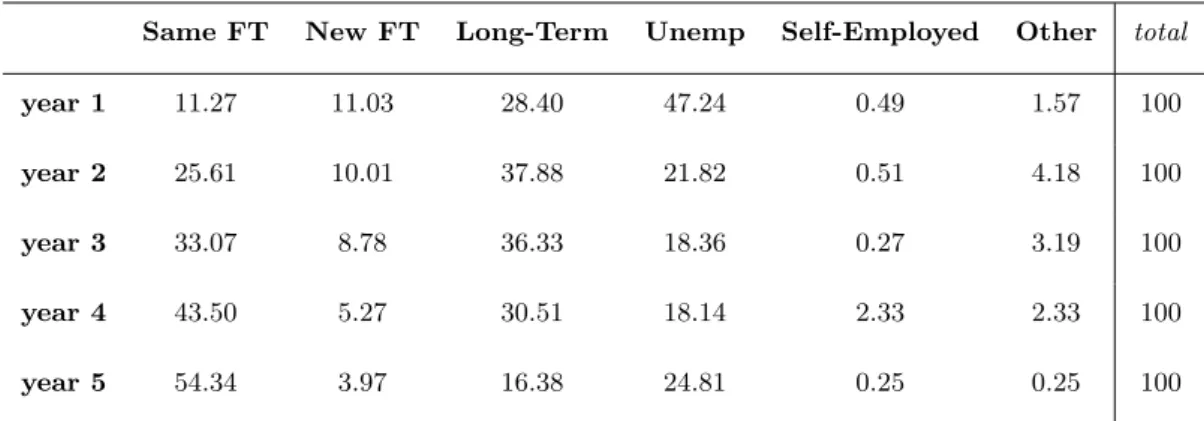
3.1 Raw yearly transition rates. 2000-2004. . . 45 3.2 Long-term conversion rates by duration and type of contract

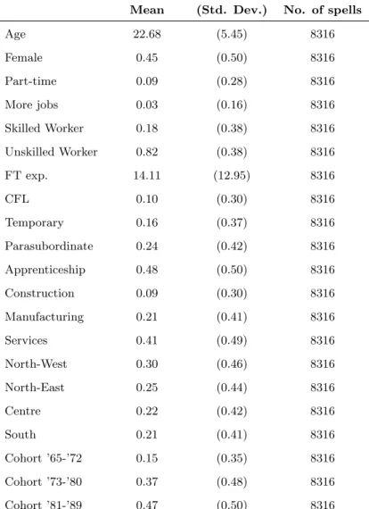
and median durations by type of contract, 2000-2004. Source: WHIP. . . 47 3.3 Mean and standard deviation of sample covariates. . . 50 3.4 Maximum likelihood estimates of the transition from fixed-term

to long-term employment: 2000-2004. . . 52 3.5 Maximum likelihood estimates of the transition from fixed-term

to long-term employment: skilled and unskilled, 2000-2004. . . 55 4.1 Summary statistics 2002-2006. . . 61 4.2 Comparison of before and after covariates. . . 65 4.3 The impact of 30/2003 reform on log of monthly wage for

fixed-term workers. . . 68 4.4 The impact of 30/2003 reform on log of monthly wage for skilled

and unskilled fixed-term workers. . . 70 4.5 Assessment of common macroeconomic shock assumption. . . . 74

(7)

Chapter 1

Introduction

In response to the dramatic rise in unemployment faced since the end of the 1970s, many European countries have made use of several policy instru-ments. On the one hand, they have been directed at relaxing the systems of employment protection by reducing the mandated costs to firms of firing workers and, on the other hand, at enhancing the use of fixed-term employ-ment contracts. Temporary workers represent a growing share of the employed workforce in many European countries. Between 1997 and 2004 the percent-age of fixed-term jobs has grown by about 2% in the EU25, reaching 13.7% in 2004 (European Commission, 2005). Each country has experienced different growth rate. The highest figures concern Spain (32.5%), Portugal (19.8%) and Poland (22.7%). The empirical evidence shows that the flows into temporary employment are all but negligible: during the nineties, over 90% of new hires in Spain have been signed under fixed-term contracts (Dolado et al., 2002; Guell and Petrongolo, 2007); in Italy, in the same period, the figure amounts to about 50% (Berton and Pacelli, 2007).

These reforms, mainly reflect a desire to maintain protections for workers in permanent jobs while giving to firms an incentive to create new, temporary jobs, which may ultimately become permanent. This is especially true for Italy, where, in the last decade, the introduction of several new contractual forms for fixed-term employment has aimed at both boosting the flexibility of the labour market and fostering job creation, leaving largely unchanged

(8)

INTRODUCTION

the legislation applying to the stock of workers employed under long-term contracts. This has given rise to a dualism in the labour market, wherein only permanent employees benefit from all the rights and job protections provided by law (see Boeri and Garibaldi, 2007; Francesconi et al., 2002).

The introduction of fixed-term contracts have raised concern among both academics and policy-makers. On the academic ground, some consensus has been achieved, namely, that intensifying the use of such contracts does not necessarily lead to an increase in employment. The effects of such a partial reform might be perverse, leading to higher unemployment, lower output and lower welfare for workers (Bentolilla and Dolado, 1994; Blanchard and Landier, 2002; Cahuc and Postel-Vinay, 2002). On the political ground, concerns are mainly about whether fixed-term contracts act as a truly ”stepping stone” to permanent employment or whether they just turn out to be a trap. It is well known that fixed-term contracts allow firms to better discriminate workers with respect to ability (see chapter 6 in Cahuc and Zylberberg, 2004): after a period of screening, firms are able to assess flawlessly workers’ ability and then decide to keep them whether talent is high enough or, conversely, to laid them off without incurring firing costs. Hence, long-term contracts may be considered as a ”reward” to the ablest workers. Ultimately, they also help to improve the quality of any match both for employer and for employee.

However, in a world with high firing costs, a substitution effect may arise. Employer might be induced by the introduction of fixed-term contracts to sub-stitute long-term jobs with fixed-term ones, since the latter are less onerous than the former and, in particular they are not subject to firing restrictions. This, in turn, may weaken the role of fixed-term contract in increasing em-ployment.

Lastly, intensive use of such contracts may also affect the fixed-term em-ployees in terms of wage raising: first, by weakening worker’s threat to quit the current temporary jobs for a better outside option (because of the absence of firing costs), and, second, by deferring any wage-tenure effect up until an open-ended contract is achieved.1

1_{This statement trivially holds for Italy, where wages raising is strictly linked to job}

(9)

INTRODUCTION

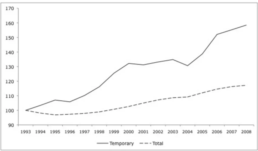
Figure 1.1: Evolution of temporary and total employment 1993-2008 (1993=100). Source: ISTAT.

The aim of my dissertation is to explore this argument, both theoretically and empirically; in particular, the goal is to shed light on the duration pattern of fixed-term contracts and the determinants of their conversion into perma-nent ones, and on the effect of temporary contracts upon wage dynamic of skilled and unskilled workers. In doing this, I focus on one country, Italy, mostly because recent introduction of such contracts and their intense use by firms has raised concerns about the effectiveness of short-term contracts to reduce unemployment and, in particular, to represent a springboard into permanent jobs. Indeed, in the last decade, young workers have been going through many spells of unemployment and low productivity short-term jobs before obtaining a regular (permanent) job, and this succession turns out to be a trap for some of them.

Fig. (1.1) depicts the evolution of fixed-term and total employment from 1993 to the second quarter of 2008, in Italy. Total employment growth is about 1.1% per year in that period; the evolution of temporary employment is even higher: the total growth amounts to 55% (3.2% on average per year). The time period 1996-2000 and 2004-2008 show the higher growth, 5.7% and 5.9% per year respectively. These remarkable increases are likely ascribed to the law 196/1997, which has introduced the agency contracts in 1998, and

(10)

INTRODUCTION

Figure 1.2: Evolution of the share of fixed-term contracts in total employment

1993-2008. Source: ISTAT.

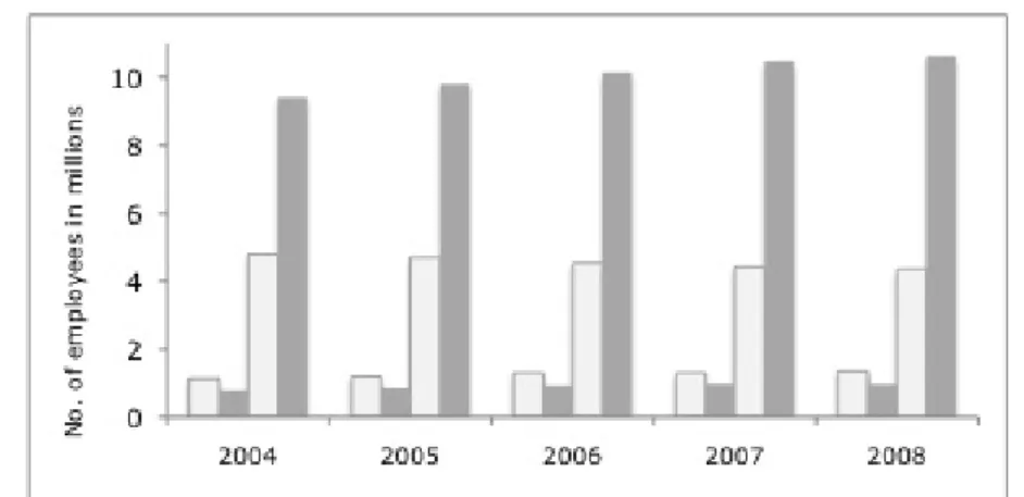
to the 30/2003, which has reformed all the previous fixed-term contracts and introduced new contractual forms (see Appendix 1 for an overview of the main features of these laws). Fig. (1.2) emphasizes this trend, showing that only between 2000 and 2004 there has been a decrease of about 1%, likely induced by the global economic slowdown. At the end of the observational period the share of fixed-term contracts amounts to 13.2%. Moreover, age is one of the main discriminant factor in the use of such contracts: 40% of workers aged under 25 and 22% of workers aged 25 to 29 is employed with a temporary contract. The opposite holds for older workers, most of them are employed with an open-ended contract (see fig. 1.3). This last figure seems to corroborate the aforementioned role of fixed-term contract, that is, a device to overcome the asymmetric information about workers’ ability. In addition, the incidence of fixed-term contracts is increasing in the educational level attained: graduate workers are more subject to be employed with a temporary contract (see for details Ministero del Lavoro, della Salute e delle Politiche Sociali, 2008).

In this work, I am interested to study how the route towards skilled (un-skilled) long-term employment can be heterogeneously affected by a change in the institutional legislation upon fixed-term contracts, pointing to create

(11)

INTRODUCTION

Figure 1.3: Evolution of temporary and total employment by age groups

2004-2008. Source: ISTAT.

more flexibility in the labour market. Moreover, concerns are also about the comprehension of how, subsequent to such a change, labour market equilib-rium alters, both in terms of unemployment rate, wage distribution and flows into and out fixed-term (long-term) employment.

The theoretical framework is based on Mortensen and Pissarides (1994), though I borrow part of the setup from Cahuc and Postel-Vinay (2002), where I introduce firing costs, learning process about workers unobservable ability and two types of contracts, fixed-term and open-ended contracts, to capture the case of interest. Moreover, I consider two submarkets, in which only jobs with a specific skill requirement and unemployed workers fulfilling such requirement participate.

The novelty is the introduction of a process of learning (screening) about workers innate ability, for only skilled positions, in the conventional matching and searching model. I treat such process as a decision theoretic optimal stop-ping problem ´a la Mortensen and Pisarrides (1999b). Knowledge of ability is achieved through successive observations of workers’ performance. Idiosyn-cratic shocks to the workers specific productivity (ability) modify the value of the match and, conditional on that, firms decide whether to continue the match or destroy it. The probability of switching contractual form, conditional

(12)

INTRODUCTION

on having observed the ability is not explicitly taken into account in the ini-tial Bellman Equations, mostly because of the desire of preserving as simple as possible the analysis of the issue. However, this simplified approach does not preclude to allow for it. It is just a matter of interpretation of the relations derived. As I consider mainly two states in which workers are employed on a temporary basis, entry level fixed-term jobs and renewed short-term jobs, it is obvious that staying in the latter presupposes that firms know the first realization, drawn from the distribution of ability. That is, they have some information about workers’ ability. This is made clearer when one looks at the key relations of the model.

Hence, in order to obtain a fixed-term contract renewal the present value of a worker’s future ability must be higher than the current one, namely, the new value of ability must be higher than the reservation value that gives rise to a non-renewal. Analogously, in order to see converted a short-term into a long-term job, the realization of ability must be higher than the reservation value that triggers a non-conversion, which, in turn, is also higher than the reservation value of a renewal. This approach enables me to uniquely identify both the determinants of job creation and destruction in terms of job specific (technology) and worker specific productivity (ability).

I further introduce an exogenous policy parameter, p, in the model which is intended to easing restrictions on the use of temporary employment contracts (e.g. renewals of fixed-term contract). Shifts in such parameter allow me to draw interesting conclusions about the key relations of the model, in particular, with respect to job creation and job destruction, equilibrium unemployment rate and wages of skilled and unskilled workers.

It will be shown that easing restrictions on the use of temporary contracts affects differently the two submarkets. In particular, in the skilled submarket, it fosters job creation, induces less frequent transformation of short-term jobs into long-term jobs and increase the within wage inequality, i.e., long-term wages push up whereas short-term wages lower for entry-level jobs and rise for the succeeding ones. One of the key effect of such a policy change is that the learning process elapses longer. This is mainly detected by the drop

(13)

INTRODUCTION

of reservation value of a renewal. Being now easier to renew contracts on a temporary basis, firms become less demanding about workers’ ability, mostly because they can now spread out the assessment about it on a longer span. This, in turn, implies that short-term jobs exhibit a lower productivity in terms of workers’ ability. At the same time, the learning process becomes more efficient: firms demand higher ability to upgrade workers with a long-term contract. As a result, it is now more likely that workers are stuck longer in short-term jobs.

Conversely, in the unskilled submarket, firms are entitled to keep short-term jobs longer (by renewing their contracts) and are more exacting about the minimum acceptable productivity, by raising the opportunity cost of long-term jobs. In addition job creation falls and wage differential between fixed-term and long-term workers decreases.

I am further able to draw some conclusion about the between wage in-equality. By comparing top earners in the skilled labor market and the bot-tom earners in the unskilled labor market, I can state that, after the policy change, the wage ratio between these two groups turn out to be wider. To some extent, an increase in p might exacerbate workers polarization in terms of earning in the economy.

The empirical analysis is aimed at recovering estimates of two main impli-cations of the model for the Italian labour market, namely, (i) the duration pattern of fixed-term contracts and (ii) the change in wages after the policy implementation. In order to allow for group-specific effects, I carry out two separate analyses for each of the issues of interest, one for skilled workers and the other one for unskilled workers (singled out along the type of occupation). The main purpose of the duration analysis is to shed light on the dura-tion pattern of fixed-term contract and in particular on the determinants of their conversion into permanent contracts. To conduct the empirical analysis I select a sample of individuals who enters the labour market via fixed-term employment over the period 2000-2004, and followed until they obtained a per-manent contract. The sample used is drawn from the WHIP dataset (Work Histories Italian Panel), which is a panel survey of individual work histories,

(14)

INTRODUCTION

based on INPS (Istituto Nazionale di Previdenza Sociale, Social Security Insti-tute) administrative archives. The model used in this empirical investigation is a continuos time duration model (Cox proportional hazard). The main find-ings can be summarized as follows: i) the probability of getting a long-term job is lower at the onset of the working career, then, it increases with the duration of the fixed-term working experience; ii) unskilled workers generally exhibit higher conversion rates than skilled ones; iii) longer span of fixed-term employment than about 48 months seems to affect negatively the transition rates.

Furthermore, irrespective of the population group considered (skilled, un-skilled workers), the highest transition rates are shown at very long durations, suggesting that on average workers have to go through a long period of fixed-term employment in order to obtain a permanent job. Had they not, they likely might even experience lower transition rates afterwards.

The goal of the second empirical investigation is to evaluate the effect of the

30/2003 law (fixed-term contract reform) on wage differentials between

work-ers employed with a short-term contract and workwork-ers with a long-term contract by skills category. I am concerned with assessing how the differential has been moving on after the introduction of the aforementioned reform. I compare the change in monthly wage of workers employed with a fixed-term contract between 2002 and 2006 in Italy to the change in monthly wage of workers employed with a long-term contract over the same period. Since the 30/2003 reform was effective starting in September 2003, I use the 2002 survey of SHIW (Survey of household income and wealth, Bank of Italy) for the before period and the 2006 survey of SHIW for the after period. To deal with it I make use of three different econometric procedure, namely basic Differences-in-differences, OLS and Difference-in-differences combined with propensity score matching. As reviewed in Abadie (2005), the DnD estimator is based on strong identify-ing assumptions. In particular, the conventional DnD estimator requires that, in the absence of the treatment, the average outcomes for the treated and control groups would have followed parallel paths over time. This assumption may be implausible if pre-treatment characteristics that are thought to be

(15)

as-INTRODUCTION

sociated with the dynamics of the outcome variable are unbalanced between the treated and the untreated. I show that all the identifying assumptions hold and thus the estimates turn out to be reliable, in particular those ones retrieved by DnD combined with propensity score matching.

Results suggests a negative impact of the reform upon fixed-term workers wages. In particular, the overall wage differential is increasing by an amount ranging 2.2% to 8.4%. When I look within skill category, i.e. skilled and unskilled workers, I validate the implications of the theoretical model. Skilled workers employed with short-term contract earn on average 22% to 36% less than skilled workers employed with long-term contract. The differential is shrinking when I consider unskilled workers.

This difference in magnitude validates the contrasting firms behaviour as implied by the theoretical model: in the skilled labor market, long-term jobs can be seen as a ’reward’ to the ablest workers and thus they have to pay more than short-term contracts. Conversely, the same does not occur (or it does but to a smaller extent) in the unskilled labor market. As unskilled jobs entail routine tasks and, thus, do not demand substantial individual ability, firms are not concerned to discern workers with respect to ability. This is corroborated by the not sizable effect of the reform on unskilled wages, as showed above.

(16)

Chapter 2

Theoretical setup

The theoretical framework is based on Mortensen and Pissarides (1994), though I borrow part of the setup from Cahuc and Postel-Vinay (2002), where I introduce firing costs, learning process about workers unobservable ability and two types of contracts, fixed-term and open-ended contracts, to capture the case of interest. Moreover, I consider two submarkets, in which only jobs with a specific skill requirement and unemployed workers fulfilling such requirement participate.

The goal of the model is to comprehend how positive change in a pol-icy, intended to easing restrictions on the use of fixed-term contract, might heterogeneously affect the labour market equilibrium, both in terms of unem-ployment rate, wage distribution and flows into and out fixed-term (long-term) employment.

In this chapter I present the model, derive the Bellman equations and characterize the equilibrium conditions for both skilled and unskilled labour market.

2.1 Preliminary Assumptions

Two types of labor contracts exist in the economy: fixed-term contracts and long-term (or open-ended) contracts. Fixed-term contracts require some predetermined duration and can be terminated at no cost, renewed for further

(17)

2.1. Preliminary Assumptions THEORETICAL SETUP

fixed period, or converted into a long-term contracts. Conversely, long-term labor contracts last as long as worker retires, and they can be terminated in any period at a fixed cost f (firing costs), incurred by the firm. For simplicity, I assume that f is equal in each submarket.

The economy has a labor force of mass one. Workers can be in either one of the following states: unemployed and searching, employed with a fixed-term contract in the first period (entry level job), employed with a renewed fixed-term contract and employed with an open-ended contract. Workers dif-fer in two aspects one observable and one unobservable to the firms. I redif-fer to the former as the educational level attained, whereas to the latter as innate ability, indicated with η. In particular, holding at least an university degree allows individuals to participate into the skilled submarket, and not holding an university degree allows to search in the unskilled submarket (submarkets are indexed by i ∈ [k, u] where k indicates skilled and u indicates unskilled).

η is a random, worker-specific productivity parameter drawn from a continuos

cumulative distribution function G(η) over the interval [ηl_{, η}h_{]. As η is} un-observable, workers look alike to the firms when they meet. Once the match starts, information about ability become less imperfect to the firms and a new value of η is drawn from its c.d.f with some probability, equals to the proba-bility that a positive job specific shock occurs. As time elapses, firms get more information about the worker ability and, then, decide to either lay off or keep him. In the following, I discuss this learning process in details. For the time being, it is worth noting that such process concerns only the case of skilled jobs, while unskilled ones are filled regardless workers ability. This assump-tion is not as strong as it appears; since I regard unskilled jobs as those which entail repetitive and routine tasks, it does make sense to expect that a high ability worker performs as much as a low ability worker. For that reason in the unskilled submarket, state in which worker (job) is employed (operating) with a renewed fixed-term contract is ruled out.

Firms freely enter the market by creating costly vacancies. Every new job is a fixed-term one. Once a vacancy is created, it may be either filled and start producing or keeping open at cost k per unit time. Without loss of generality,

(18)

2.1. Preliminary Assumptions THEORETICAL SETUP

I assume that k is equal in both submarkets.

Vacant jobs and unemployed workers meet at rate determined by the ho-mogeneous of degree one matching function m(vi, ui), where vi is the num-ber of vacancies and ui is the number of unemployed workers in submar-ket i. In particular, a vacant job can meet an unemployed worker at rate

m(vi, ui)/vi = q(θi) with q"(.) < 0, a decreasing function of θi. Similarly, a job seeker can meet a vacant job at rate θiq(θi), an increasing function of θi. θi indicates the labor market tightness ratio in each submarkets i.

It is worth pointing out that not all job contacts will be filled and start pro-ducing as in the Mortensen and Pissarides (1994) original model. In Cahuc and Postel-Vinay’s model (2002) it is assumed that some jobs may not be productive enough to start producing; as the starting value of productivity is revealed just after the match is formed, it may be too low to compensate worker and employer for their search effort. Following them somehow, I as-sume that firms decide to transform contacts in jobs with some probability. More precisely, my assumption is slightly different from that one of Cahuc and Postel-Vinay. Instead of assuming, as they do, that every type of job (short-term, new long-term and continuing long-term job) comes along with its specific value of productivity, I suppose that JOB has a specific level of productivity, no matter which labor contract entails. Thus, rather than treat-ing every type of contract as different job, I think of contracts as alternatives of the same job position. Where does exactly such probability comes from will be clear when I derive the Bellman equations.

Once a position is filled, production takes place. The firm’s output per unit of time is ε + η, where ε is a job specific component and η is worker specific. ε is a random job specific productivity parameter drawn from a con-tinuos cumulative distribution function F (ε), and probability density function

f (ε) over the interval [ε, ¯ε]. Firm may be hit by a shock with instantaneous

probability δ, that changes the job specific productivity; a new value of the job is drawn from its c.d.f. F (ε).

(19)

2.2. The learning process THEORETICAL SETUP

2.2 The learning process

As mentioned above, in the skilled submarket firms are also concerned with workers innate ability. Given that fixed-term contracts may be interrupted at any point in time at no cost, it enables firms to evaluate the level of workers ability when they are employed. After observing ability, firms decide whether to keep or dismiss workers when his/her level is above or below some critical value respectively. Fixed-term jobs de facto reduce the risk of uncertainty about worker’s ability borne by firms.

I consider a learning process wherein learning about the expected produc-tivity of particular workers is achieved through successive observations of their performance. Even though the learning process implemented in the model in-volves both agents, I prefer to stress the employer side of the process, because it makes assumptions more easily-seized. However, it is not awkward to think that even workers might be concerned to learn about their unobservable traits, in order to sort away from things that they do poorly.

Knowledge of ability is achieved through successive observations of work-ers’ performance and such observations refer to workwork-ers’ performance in dif-ferent tasks per period. When the match starts, workers are ex ante similar in terms of ability to the firms. After one period of employment, having ob-served how the worker performs in some tasks, firm grasps some information that allows for a first evaluation of worker’s ability. Such information is not adequate to unambiguously assess his/her level of ability, but enough to de-cide whether quitting or renewing with another fixed-term contract the match. Through successive steps, information become less and less noisy and a thor-ough appraisal upon workers’ ability is achieved. By means of that, then, the conversion of temporary jobs into long-term jobs is determined. I deal with such process as a decision theoretic optimal stopping problem ´a la Mortensen and Pisarrides (1999b). These successive stages are detected by idiosyncratic shocks to the workers specific productivity (ability). Idiosyncratic shocks mod-ify the value of the match and, conditional on that, firms decide whether to continue the match or destroy it. The probability of switching contractual form, conditional on having observed the ability is not explicitly taken into

(20)

2.2. The learning process THEORETICAL SETUP

account in the initial Bellman Equations, mostly because of the desire of pre-serving as simple as possible the analysis of the issue. However, this simplified approach does not preclude to allow for it. It is just a matter of interpretation of the relations derived. As I consider mainly two states in which workers are employed on a temporary basis, entry level fixed-term jobs and renewed short-term jobs, it is obvious that staying in the latter presupposes that firms know the first realization, drawn from the distribution of ability. That is, they have some information about workers’ ability.

Hence, in order to obtain a fixed-term contract renewal the present value of a worker’s future ability must be higher than the current one, namely, the new value of ability must be higher than the reservation value that gives rise to a non-renewal. Analogously, in order to convert a short-term into a long-term job, the realization of ability must be higher than the reservation value that triggers a non-conversion, which, in turn, is also higher than the reservation value of a renewal. This fact is pinpointed by relations (2.17) and (2.18) in the following. I will show that there exist reservation ability values below which the employer does not want to keep the worker neither with a fixed-term nor with a long-term contract. I pinpoint two values of interest, one for each type of contract.

It is worth pointing out that this process presupposes that job specific productivity is not below some critical value. When negative productivity shocks have not still occurred, the learning process takes place, otherwise the issue turns out to be pointless. The assumption is that job specific productivity shock prevails over worker specific one. The rationale is straightforward: why firms has to be concerned with worker ability when job is not productive enough per se? Employers do not actually care about screening whether there is no positive surplus from the trade. Thus, in that case, jobs are simply destroyed. This is taken into account by imposing that the draw of a new value of η takes place with some probability that a positive job specific shock occurs.

Furthermore, I put a condition on the renewals of fixed-term contract by means of the assumption that any renewals must be provided by law.

(21)

Con-2.3. Skilled labor market THEORETICAL SETUP

sequently a fraction p of the fixed term jobs may be renewed with another fixed-term contract, otherwise, whether the firm agrees, they must be turned to a long-term one. p is interpreted as a policy instrument.

2.3 Skilled labor market

In the skilled submarket employers and workers meet following the afore-mentioned matching function m(uk, vk). Decisions about opening a vacancy, destroying an existing job, being unemployed and employed are characterized by the customary Bellman equations. I denote by Jki, Wki, Uk, Vkthe value of a filled job, of being employed, of being unemployed and of a vacancy respec-tively, where index i ∈ [s, r, p] indicates the type of labor contract, s stands for short-term in the first period, r for renewed short-term and p for long-term.

Before deriving the Bellman equations, I define the total surplus of the match to the pair, associated with each type of job, as the sum of the values of the above value functions:

S_ki(η, ε) = J_ki(η, ε) − Vk(η, ε) + Wki(η, ε) − Uk(η, ε) for i = s, r

S_kp(η, ε) = J_kp(η, ε) − [Vk(η, ε) − f] + W_kp(η, ε) − Uk(η, ε)

The difference between those surpluses is represented by firing costs. They only enters the total surplus of the long-term job, because firm incurs firing costs upon destroying it.

Match rents are divided between firm and worker by the generalized Nash wage rule, with continuous renegotiation, i.e.:

J_ki(η, ε) − Vk(η, ε) = βSki(η, ε) for i = s, r (2.1)

J_kp(η, ε) − [Vk(η, ε) − f] = βSkp(η, ε) (2.2) where β ∈ [0, 1] indicates the firm bargaining power.

(22)

2.3.1. Bellman equations THEORETICAL SETUP

2.3.1 Bellman equations

A long-term contract returns a flow of output equal to ε + ¯η and pays a wage wp _{per unit of time. η is taken as a constant because the screening about} worker ability has already taken place. Long-term job may be hit by a shock with instantaneous probability δ that changes the job specific productivity. Having observed the new value of ε, the firm and the worker decide whether to keep alive the match or to destroy it at a fixed cost f. Thus, the values of filling a long-term job and of being employed with a long-term contract are given by the following Bellman equations (from now on I omit the subscript

k to make notations clearer):

rJp(ε, η) = (ε + ¯η) − wp+ δ ! {max[Jp(x, η), V − f] − Jp(ε)}dF (x)(2.3) rWp(ε, η) = wp+ δ ! {max[Wp(x, η), U] − Wp(ε)}dF (x) (2.4)

A renewed short-term contract returns a flow of output equal to ¯ε+ η and pays a wage wr _{per unit of time. As I assume that the learning process does} take place only when job specific productivity is not below some critical value,

ε is taken as a constant. Information about workers’ ability becomes less

noisy as time goes by, and a new value of η is drawn from its c.d.f G(η) with probability [1 − F (ε∗)]. Having observed the new value of η, the firm and the worker decide whether to continue the match as a long-term job or to destroy it at no cost and go back to the search market. Thus, the values of filling a renewed short-term job and of being employed with a renewed short-term contract are given by the following Bellman equations:

rJr(ε, η) = (¯ε+ η) − wr+ [1 − F (ε∗)] ! {max[Jp(ε, x), V ] − Jr(ε, η)}dG(x) −F (ε∗)[Jr(ε, η) − V ] (2.5) rWr(ε, η) = wr+ [1 − F (ε∗)] ! {max[Wp(ε, x), U] − Wr(ε, η)}dG(x)

(23)

−F (ε∗)[Wr(ε, η) − U] (2.6)

A short-term (entry-level) job returns a flow of output equal to ¯ε+ η and pays a wage ws _{per unit of time. ε is constant, the same arguments as before} apply. Then, conditional on the new value of η, the firm and the worker decide whether to continue the match or destroy it at no cost and go back to the search market. A fraction p of these matches is renewed with another fixed-term contract and a fraction 1 − p is converted into long-term job. The value to the firm and to the worker of an entry-level job solves the following Bellman equations: rJs(ε, η) = (¯ε+ η) − ws+ [1 − F (ε∗)] " p ! {max[Jr(ε, x), V ] − Js(ε, η)}dG(x) + (1 − p)! {max[Jp(ε, x), V ] − Js(ε, η)}dG(x) # −F (ε∗)[Js(ε, η) − V ] (2.7) rWs(ε, η) = ws+ [1 − F (ε∗)] " p ! {max[Wr(ε, x), U] − Ws(ε, η)}dG(x) + (1 − p) ! {max[Wp(ε, x), U] − Ws(ε, η)}dG(x) # −F (ε∗)[Ws(ε, η) − U] (2.8)

Firms freely enter the market by creating costly vacancies. A vacancy is kept open at cost k per unit of time, whereas is filled at rate q(θ) with probability [1 − F (ε∗_{)]. Every new job is a fixed-term one. When meet a} worker, a firm decides to hire a worker if the value of a filled short-term job is greater than the value of keeping the slot vacant. The job specific productivity

ε de facto reveals the profitability of such a choice. The value of a vacancy is

(24)

2.3.2. The Equilibrium THEORETICAL SETUP

rV = −k + q(θ)[1 − F (ε∗)][Js(ε, η) − V ] (2.9)

A job seeker benefits from a flow of exogenous value of leisure or unem-ployment income b when unemployed. She/he comes in contact with a vacant short-term job at rate θq(θ) with probability [1 − F (ε∗_{)]. The value of} unem-ployment to the worker solves the following Bellman equation:

rU = b + θq(θ)[1− F (ε∗)][Ws(ε, η) − U] (2.10)

Having derived the Bellman equations for each of the three states, I now turn to characterize the equilibrium conditions.

2.3.2 The Equilibrium

An easy way to derive the equilibrium is first to rewrite the value functions in terms of surplus, with the help of the sharing rules (2.1) and (2.2), then identify the threshold values of productivity and ability as functions of the labor market tightness θ.

Firms post vacancies on the assumption of free entry in the market. Be-cause of free entry, the value of a vacancy must always be equal to zero in equilibrium. From (2.9) and the sharing rule (2.1), I get the following equal-ity:

k

q(θ)[1_{− F (ε}∗_)]β = S

s _(2.11)

Substituting this relation into equation (2.10), adding it up toghether with the Bellman equations (2.3) - (2.8) and making use of the specific sharing rule, one ends up with expressions of the total match surpluses as follows:

(25)

2.3.2. The Equilibrium THEORETICAL SETUP −1 − β β kθ (2.12) (1 + r)Sr_{(ε, η) = (¯ε+ η) − b + [1 − F (ε}∗_)]! _max[Sp_{(ε, x), 0]dG(x)} −1 − β β kθ (2.13) (1 + r)Ss_{(ε, η) = (¯ε+ η) − b + [1 − F (ε}∗_)]"_p! _max[Sr_{(ε, x), 0]dG(x)} (1 − p)! max[Sp_{(ε, x), 0]dG(x)} # −1 − β_β kθ (2.14)

As each of the above surpluses are monotonically increasing in their current job specific or worker specific productivity parameters (depending on which surplus one is looking at), job destruction satisfies a reservation property. There exists a unique reservation job specific (worker specific) productivity value which makes surplus to drop to zero. As a result, a long-term job that get a job specific productivity shock ε <ε ∗ _{is destroyed, where ε}∗ _{is given} by Sp_(ε∗_{) = 0. Similarly, a renewed short-term job is not transformed into} a long-term one whether observed worker ability is not at least equal to ηc_, coming from Sr_{(¯ε, η}c_{) = 0, and a short-term labor contract is not renewed} with another short-term contract whether observed worker ability is not at least equal to η∗_{, where η}∗ _{is given by S}s_{(¯ε, η}∗_{) = 0. Note that in case of a} new or renewed short-term job, ε >ε∗ _{must also be satisfied, otherwise job is} destroyed straightaway.

Thus, imposing the condition Sp_(ε∗_{) = 0 and solving the integral term,} the equation (2.12) can be expressed as follows:

(ε∗_{+ ¯η) − b + f + δ}! ¯ε ε∗

Sp"(x)[1 − F (x)]dx − 1 − β

β kθ = 0

Noting from equation (2.12) that Sp"_{(x) = 1/r + δ I obtain the following}

relation: (ε∗_{+ ¯η) = b +}1 − β β kθ− f − δ r + δ ! ¯ε ε∗[1 − F (x)]dx (2.15)

(26)

This is one of the key conditions of the model. It relates the job specific reservation productivity to labor market tightness. As in Mortensen and Pis-sarides (1994) ε∗ _{is increasing in the ratio of vacancies to unemployment, θ.} The rationale behind this upward sloping is well known: briefly, more vacan-cies than unemployed workers increase the value of being unemployed, because now it is easier to find a job; the higher the value of U, the lower the value of the total surplus, hence match productivity must increase in order to com-pensate agents for their outside options. Furthermore, as in Mortensen and Pissarides (1999), keeping θ constant, it is easily established by differentiation that ε∗ _{decreases with f, namely, an increase in f reduces job destruction in} equilibrium; this is de facto what the firing costs aim at. With no particular fancy, I refer to this as the firing relation (FR).

Applying the condition Sr_{(¯ε, η}c_{) = 0 to equation (2.13) and following the} same procedure as before, the second condition of the model comes out:

(¯ε + ηc_{) − b + [1 − F (ε}∗_)]! η

h

ηc

Sp"(x)[1 − G(x)]dx −1 − β

β kθ = 0

Note from definition of Sp_(ε∗_{) that, since η enters as a constant, its} deriva-tive with respect to η is zero, so the integral term drops to zero and I end up with the following:

(¯ε+ ηc_{) = b +}1 − β

β kθ = 0 (2.16)

This relation gives the worker specific reservation productivity (ability) in terms of the labor market tightness parameter, holding ε constant. More precisely, it makes ηc _{an increasing function of θ. The intuition is as before: a} tighter labor market rises the value of U; this lower the total match surplus, hence, for a given ε, worker specific productivity must rise to offset the increase of agents’ outside options. I refer to this relation as the Upgrading Relation (UR), because it provides the critical value of worker ability that make firms indifferent between upgrading the worker with a renewed short-term contract to a long-term job and laying him/her off.

(27)

The third condition of the model arises employing Ss_{(¯ε, η) = 0 to the} equation (2.14). Recalling that ∂Sp_{(ε)/∂η = 0 and ∂S}r_{(¯ε, η)/∂η = 1/1 + r, I} get the following expression:

(¯ε+ η∗_{) = b +} 1 − β β kθ− F (ε∗)p 1 + r ! ηc η∗ [1 − G(x)]dx (2.17) I call this the continuing short-term relation (CSTR). It is an increasing function of the labor market tightness parameter, keeping ε constant. It pin-points a cutoff level of worker ability η∗ _{below which a short-term job is not} perpetuated as a renewed short-term job. The same arguments of equation 2.17 apply.

In order to get a more compact and analytically more convenient form of the upgrading relation, subtract the CSTR from (2.16) to get:

ηc = η∗+F (ε∗)p

1 + r ! ηc

η∗ [1 − G(x)]dx (2.18)

Equation (2.18) facilitates comparison between the upgrading relation and the continuing short-term relation. It first clarifies the ranking of threshold values of worker specific productivity, that is ηc _{is greater than η}∗_{; second,} it shows how the policy p (of allowing short-term contract renewals) affects the job dismissal behaviour of the firms. With p = 0, the distinction between short-term and renewed short-term contracts vanishes, as a result only ηc _is crucial in making decision about dismissals. From now on, equation (2.18) will be used as the upgrading relation instead of equation (2.16).

The last relation left to be derived is the job creation rule (JC). It is easily obtained by substituting equation (2.14) into (2.11), noting that (2.14) can be written down as Ss_{(¯ε, η) − S}s_{(¯ε, η}∗_{) = η − η}∗_{/1 + r:}

q(θ) = (1 + r) β[1− F (ε∗_)]

k

η− η∗ (2.19)

For a given value of ε∗_{, labor market tightness is decreasing in η}∗_. Analo-gously, for given η∗_{, labor market tightness is decreasing in ε}∗_{. In both cases}

(28)

the intuition is straightforward: the lower the destruction threshold, the higher the expected return of a match. As jobs last longer, firms tend to post more vacancies.

It is worth pointing out, unlike Mortensen and Pisarrides (1999), that firing costs do not enter and seem not to affect directly job creation equation. This is ascribed to the assumptions of the model. Bring to mind that vacancies are only filled with fixed-term jobs, thus firing costs should not apparently affect job creation behaviour of firms (in terms of reducing vacancies posted) because such costs only apply to long-term jobs. Conversely, what it is apparent from equation (2.19) is that more stringent firing restrictions, lowering the value of

ε∗, increase the initial expected present value of jobs; in turn, this gives rise

to a larger vacancy creation.

The joint determination of θ, ε and η in the skilled labor market is depicted in figure 2.1. The way how the relations are drawn needs some discussion. First, note that job creation rule is a function of both ε∗ _{and η. It can be easily} shown by differantiation that it is a decreasing function of both parameters. The proof is as follows:

Proof. Differentiating equation (2.19) with respect to q(θ) and ε∗_{, one gets:} dq(θ) dε∗     η∗_=const = (1 + r)f(ε∗)k β(η_{− η}∗_{)[1 − F (ε}∗_)]2 > 0

Recalling that q"_{(θ) < 0, it is evident that θ is decreasing in ε}∗_.

This result allows to draw the job creation rule downward sloping in the upper panel of fig. 2.1, for given value of η∗_{. JC moves in the (ε}∗_{, θ) plane} as η∗ _{varies, that is, larger (lower) values of η}∗ _{shifts the JC curve to the left} (right).

Yet, differentiating equation (2.19) with respect to q(θ) and η∗_{, one gets:} dq(θ) dη∗     ε∗=const = (1 + r)k β[1− F (ε∗_{)](η − η}∗₎2 > 0 θ is decreasing in η∗, as required.

The bottom of fig. 2.1 displays the job creation curve in the (η∗_{, θ) plane.} Note that JC is drawn for given value of ε∗_{, that means that an increase} (decrease) of ε∗ _{shifts JC curve to the left (right).}

(29)

Having disentangled this point, I am now able to illustrate the joint de-termination of all the parameters of the model. The JC and FR in panel (a) of fig. 2.1 uniquely determine the value of the reservation job specific pro-ductivity ε∗_{, and the labor market tightness θ}∗_{. θ}∗ _{is also identified with the} intersection between JC and CSTR in panel (b). This, in turn, determines the threshold value of worker specific productivity η∗_{. Finally, substituting θ}∗ into the upgrading relation, ηc _{is unambiguosly identified (it is shown as the} intersection of UR and the straight line going through θ∗_).

Wages

Wage is the outcome of bilateral bargaining between firms and workers. They share the quasi-rent by the generalized Nash rule (2.1) and (2.2), as a result the wage is derived as follows:

wi = arg max(Ji(ε, η) − V )β(Wi(ε, η) − U)1−β for i = s, r

wp = arg max(Jp(ε) − V + f)β(Wp(ε) − U)1−β

Substituting the relevant value functions into the above conditions provides the expressions of wages for each type of contract:

ws = βb + (1 − β)[¯ε+ η + kθ)] (2.20)

wr = βb + (1 − β)[¯ε+ η + kθ)] (2.21)

(30)

Figure 2.1: The joint determination of θ, ε and η in the skilled labor market

ε∗ η∗ ηc θ∗ θ∗ a) b) !!!! !!!! !!!! !!!! !!!! !!!! !!!! !!!! !!!! !!!!F R CST R U R " " " " " " " " " " " " " " " " "" " " " " " " " " " " " " " " " " "" JC JC !!!! !!!! !!!! !!!! !!!! # # ε η $ $ θ θ

The above expressions are quite standard. Although ws_{and w}r _{look alike,} they differ in the value of η. It is inferred that the wage paid by a renewed

(31)

short-term job is identified for values of η over the interval [η∗_{, η}c_{], and that} one paid by an entry-level job for values of η < η∗_.1 _{As well as be increasing}

in ε and identified for given values of η, wp _{takes also into account the firing} costs. Workers can use them as an additional threat in wage bargaining and, as a result, a long-term job pays a higher wage. Thus, the ranking of the wages for each type of job is wp _{> w}r_{> w}s_.

Unemployment

I complete the steady state analysis by deriving the equilibrium value of unemployment rate.

The total number of workers employed with an entry-level job amounts to θq(θ)[1 − F (ε∗_{)]u; a fraction p[1 − G(η}∗_{][1 − F (ε}∗_{)] of which is renewed} with another fixed-term contract and a fraction (1 −p)[1−G(η∗_{)][1 −F (ε}∗_{)] is} converted into a long-term job. Among entry-level short-term jobs, those with worker specific productivity less than η∗ _{and a fraction F (ε}∗_{) (i.e., jobs with} job specific productivity less than ε∗_{) are terminated. Analogously, among} renewed short-term jobs, those with worker specific productivity less than ηc and a fraction [1 − F (ε∗_{)] are destroyed (i.e., not transformed into long-term} ones). Adding up the fraction (1 − p) of entry-level short-term jobs and the number of jobs coming from renewed short-term contracts, one gets the total number of long-term jobs in the economy. A fraction δF (ε∗_{) of those jobs are} destroyed every period. Therefore, the evolution of unemployment is given by the following apparently cumbersome equation:

˙u = [1 − F (ε∗_{)]θq(θ)u + [1 − F (ε}∗_{)][1 − G(η}∗_{)]p[1 − F (ε}∗_)]θq(θ)u

+[1 − F (ε∗_{)][1 − G(η}c_{)](1 − p)[1 − F (ε}∗_)]θq(θ)u

1_{Equation (2.39) actually does not explain which value of η has to be considered and,}

recalling that firms and workers are uncertain about workers ability, it seems that η should not be really taken into account in the determination of such wage. In spite of that and as far as the model tells, I can infer that such value must be less than η∗.

(32)

2.3.2. The Equilibrium THEORETICAL SETUP +[1 − F (ε∗_{)][1 − G(η}c_{)][1 − F (ε}∗_{)][1 − G(η}∗_{)]p[1 − F (ε}∗_)]θq(θ)u −F (ε∗)θq(θ) − [1 − F (ε∗)]G(η∗)θq(θ)u − [1 − F (ε∗)]G(ηc)[1 − F (ε∗)] [1 − G(η∗_{)]p[1 − F (ε}∗_{)]θq(θ)u − δF (ε}∗₎ % 1 − u − [1 − F (ε∗_{)]θq(θ)u +} [1 − F (ε∗_{)][1 − G(η}∗_{)]p[1 − F (ε}∗_)]θq(θ)u &

In steady state inflows into unemployment must be equal to outflows, as a result the equilibrium unemployment rate is:

u∗ = δF (ε∗)/[1 − F (ε∗)] δF (ε∗_{)/[1 − F (ε}∗_{)] + θ}∗_q(θ∗₎ % [1 − G(η∗_{)] + [1 − G(η}c_)]− ... δF (ε∗_{) − δF (ε}∗_{)/[1 − F (ε}∗_{)] + p} ' 1 − G(η∗_{) − [1 − G(η}c)]+ ... [1 − G(η∗_{)][1 − G(η}c_{) − (1 − δ)F (ε}∗_{) − G(η}c₎ (& (2.23) The above expression shows the familiar increasing relation between equi-librium unemployment rate and job specific reservation productivity ε∗_{; in} terms of the model this means that, ceteris paribus, the higher the value of

ε∗ the higher the destruction rate of long-term jobs. Unemployment also rises

whether firms are more demanding about workers ability, both for renewing a short-term contract, η∗_{, and for upgrading jobs into long-term ones, η}c_{, other} things equal. Unfortuntely the interpretation of p, the policy instrument that allows contracts renewals, is not so clear-cut. As p depends on the sign of the

(33)

2.3.3. Comparative statics THEORETICAL SETUP

terms in round brackets in (2.23), which is not of immediate interpretation, it is ambiguously related to u∗_{. However, I can say more about it in the next} section.

2.3.3 Comparative statics

Having derived the key relationships of the economy, it is simple to examine the effect of a change in one of the parameters. What I am interested in, is the net effect of changes in the policy instruments p on the hiring and and firing behaviour of the firms. Put it differently, how do less stringent restrictions on short-term contract renewals affect the labor market equilibrium? The answer to this question can be easily obtained by doing some comparative static to the model. The effect of an increase in p on job creation and job destruction is sketched in figure (2.2).

An increase in p shifts the CSTR downward: short-term jobs last longer on average (i.e., they are perpetuated with another short-term contract more frequently) which raises their expected present value; for a given θ, an increase in p lowers η∗_{. The intuition is that, as it is easier to renew a short-term} contract, the learning process about her/his productivity is spread out on a longer span; firms are less exacting on the level of η required to renew the contract.

The UR shifts upward: for a given θ, an increase in p induces less frequent transformation of renewed short-term jobs into long-term jobs. As the learning process elapses longer, assessment about workers ability is now more efficient (compared to situation in which renewal were not allowed), hence, firms ask for larger value of η to upgrade workers with a long-term contract . Accordingly, firms better offset expensive termination of long-term jobs.

In order to take into account the decrease of η∗_{, the JC curve in panel (a)} shifts to the right (recall that JC is drawn for given value of η∗_{, see discussion} above) and a new value of labor market tightness is detected. Thus job creation increases. Moreover, note that JC in panel (b) does not move because p does affect JC only through its effect on η∗_{, which it is already taken into account} by shifting in θ∗_{. The proofs of these statements follow.}

(34)

Figure 2.2: The effect of an increase in p in the skilled labor market

ε∗ η∗ ε∗! η∗! ηc ηc! θ∗ θ∗ θ∗! θ∗! a) b) !!! !! !! !! !! !! !! !! !!! !! !!! !! !! !! !! !! !! !!!F R CST R U R " " " " " " " " " " " " " " " " "" " " " " " " " " " " " " " " " " "" JC JC !! !!! !! !! !! !! !! !! !!! !!!! !!!! !!!! !!!! !!!!CST R! !!!! !!!! !!!! !!!! ! U R! " " " " " " " " " " " " " " " " "" JC! # # ε η $ $ θ θ

Proof. Differentiating equation (2.17) with respect to η∗ _{and p, one gets:} dη∗ dp     = − (F (ε∗₎)ηc η∗[1 − G(x)]dx 1 + r + F (ε∗_{)[1 − G(η}∗_)] < 0

(35)

2.4. Unskilled labor market THEORETICAL SETUP

Hence η∗ _{is decreasing in p.}

Yet, differentiating equation (2.18) with respect to ηc _{and p, one gets:} dηc dp     θ=const = − * dη∗ dp     θ=const −(F (ε_{1 + r}∗)p ! ηc η∗ [1 − G(x)]dx + > 0 Hence ηc _{is increasing in p.}

I can be more precise about the shift of UR. Note from the proof above that the differential dηc_{/dp is greater than dη}∗_{/dp, thus the shift of UR is} larger than the shift of CSTR: it is now harder to get a long-term job! More interesting, the shift of JC in panel (a) picks a new value of the reservation job specific productivity ε∗_{. The opportunity cost of long-term jobs (of every jobs} actually) raises leading to more intense job turnover. It is now more likely that, throughout their career, workers are stuck longer in short-term jobs. Analogously, the increase in ε∗ _{might reflect firms’ propensity to substitute} long-term jobs with short-term jobs.

As both job creation and job destruction increase in equilibrium, the effect of an increase in p on the unemployment rate looks ambiguous. However, both in terms of job specific, ε∗_{, and worker specific productivity, η}c_{, job destruction} increases more compared to the increase in job creation, as a result equilibrium unemployment rate rises.

2.4 Unskilled labor market

Workers who do not hold an university degree are entitled to search in the

unskilled submarket. In this submarket, firms are not concerned in learning

about workers ability, as a result the hypothesis about the learning process is discarded (see above for the rationale behind such a premise). However, the distinction between short-term jobs and long-term jobs is still relevant. In particular, firms post vacancies only as short-term jobs. Derivation of the Bellman equations and characterization of the equilibrium follow.

In the unskilled submarket employers and workers meet following the matching function m(uu, vu). I denote by Jui, Wui, Uu, Vu the value of a filled

(36)

job, of being employed, of being unemployed and of a vacancy respectively, where index i ∈ [s, p] indicates type of labor contract, s stands for short-term and p for long-term.

Match rents are divided between firm and worker by the generalized Nash wage rule, with continuous renegotiation, i.e.:

J_us(ε) − Vu(ε) = β[Jus(ε) − Vu(ε) + Wus(ε) − Uu] (2.24)

J_up(ε) − [Vu(ε) − f] = β[Jup(ε) − Vu(ε) + f + Wup(ε) − Uu] (2.25)

where β ∈ [0, 1] indicates the firm bargaining power.

The difference between those equation is again represented by firing costs. They only enters the total surplus of the long-term job, because firm incurs firing costs upon destroying it.

2.4.1 Bellman equations

A new short-term job returns a flow of output equal to ε + ¯ηu and pays a wage ws

u per unit of time. Under the assumptions of the model, ηu is taken as a constant. Short-term jobs may be hit by a shock with instantaneous probability δ, which changes the value of ε. It is drawn from its c.d.f F (ε). Then, a fraction (1 − p) of these matches are perpetuated as long-term job. The value of a new short-term job to the firm and to the worker solves the following Bellman equations:

rJ_us(ε) = (ε + ¯ηu) − wsu+ (1 − δ)p[Jus− Vu] + (1 − p)δ ! {max[Jup(x), Vu] − Jus(ε)}dF (x) (2.26) rW_us(ε) = w_us+ (1 − δ)p[W_us_{− U}u] + (1 − p)δ ! {max[Wup(x), Uu] − Wus(ε)}dF (x) (2.27) where Jp

(37)

2.4.2. Equilibrium THEORETICAL SETUP

worker under the open-ended contract. These value functions solve the follow-ing functional equations:

rJ_up(ε) = (ε + ¯ηu) − wpu+ δ ! {max[Jup(x), Vu− f] − Jup(ε)}dF (x)(2.28) rW_up(ε) = w_up+ δ ! {max[Wup(x), Uu] − Wup(ε)}dF (x) (2.29)

Firms freely enter the market by creating costly vacancies. A vacancy is kept open at cost k per unit of time, whereas is filled at rate q(θu). Every new job is a fixed-term one. When meeting a worker, a firm decides to hire a worker if the value of a filled short-term jobs is greater than the value of keeping the slot vacant. The value of a vacancy is given by the following Bellman equation:

rVu = −k + q(θu)[Jus(ε) − Vu] (2.30) A job seeker benefits from a flow of exogenous value of leisure or unem-ployment income bu when unemployed. She/he comes in contact with a va-cant short-term job at rate θuq(θu). The value of unemployment to the worker solves the following Bellman equation:

rUu = bu+ θuq(θu)[Wus(ε) − Uu] (2.31)

2.4.2 Equilibrium

Like in the skilled labor market I first rewrite the value functions in terms of surplus, with the help of the sharing rules (2.24) and (2.25), then I derive the threshold values of productivity as functions of the labor market tightness

θu.

Because of free entry, the value of a vacancy must always be equal to zero in equilibrium. From (2.30) and the sharing rule (2.24), I get the following equality:

(38)

k q(θ)β = S

s _(2.32)

Substituting this relation into equation (2.31), adding it up toghether with the Bellman equations (2.26) - (2.29) and making use of the sharing rule (2.24), one ends up with expressions of the total match surpluses for the short-term and long-term jobs as follows:

(1 + r + δp)Ss u(ε) = (ε + ¯ηu) − bu+ (1 − p)δ ! max[Sp u(x), 0]dF (x) − 1 − β_β kθu (2.33) (r + δ)Sp u(ε) = (ε + ¯ηu) − bu+ f + δ ! max[Sp u(x), 0]dF (x) − 1 − β_β kθu (2.34) Each of the above surpluses are monotonically increasing in their current job specific productivity parameter, that means that job destruction satisfy a reservation property. There exists a threshold productivity which make surpluses equal to zero.

Thus, imposing the condition Sp

u(εc) = 0 and solving the integral term, one gets the threshold value εc _{as follows:}

(εc_{+ ¯η} u) = bu+1 − β β kθu− f − δ r + δ ! ε¯ εc[1 − F (x)]dx (2.35) I refer to this relation as the Firing Relation (FR). It makes the threshold productivity εc _{an increasing function of the unskilled labor market tightness} parameter θu.

Similarly, I derive the threshold value that triggers a short-term dismissal as follows: (ε∗_{+ ¯η} u) = bu+1 − β β kθu− (1 − p)δ r + δ ! ε¯ εc[1 − F (x)]dx (2.36)

(39)

ε∗ = εc+ f + pδ r + δ

! ε¯

εc[1 − F (x)]dx (2.37)

I call this relation the Upgrading Relation (UR) (in line with the its ”coun-terpart” in the skilled submarket), because it provides the reservation pro-ductivity of the match which makes firms and workers indifferent between upgrading the match with a long-term job and destroy it.

The job creation rule is obtained by substituting (2.33) into (2.32) and noting that (2.33) can be written down as Ss_{(ε) − S}s_{(ε∗) = ε − ε}∗_{/(r + δ):}

q(θu) =

k β

r + δ

(ε − ε∗₎ (2.38)

As in the conventional Mortensen an Pissarides’ model, labor market tight-ness is decreasing in εc_{. The lower the destruction threshold, the higher the} expected return of a match: jobs last longer, thus, firms tend to post more vacancies.

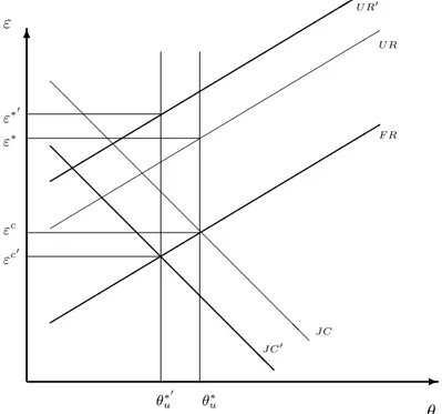
The joint determination of θu, ε∗ and εc in the unskilled labor market is depicted in figure 2.3. Substituting the value for ε∗ _{defined in equation (2.37)} into JC and using FR, the labor market tightness θ∗

u is uniquely determined. In turn, ε∗ _{is characterized directly from UR.}

Wages

The Nash wage bargain is a contingent wage contract defined by:

ws = arg max(J_us(ε) − Vu)β(Wus(ε) − Uu)1−β

wp = arg max(J_up(ε) − Vu+ f)β(Wup(ε) − Uu)1−β

Substituting the relevant value functions into the above conditions provides the expressions of wages for each type of contract:

(40)

Figure 2.3: The joint determination of θu, ε∗ and εc in the unskilled labor

market εc ε∗ θ∗ u !!!! !!!! !!!! !!!! !!!! F R U R " " " " " " " " " " " " " " " " ""JC !!!! !!!! !!!! !!!! !!!! # ε $ θu ws_u = βbu+ (1 − β)[ε + ¯ηu+ kθu)] (2.39) wp_u = βbu+ (1 − β)[ε + ¯ηu+ kθu)] + (1 − β)f (2.40) Unemployment

The final equation of the model is the steady state condition for unem-ployment. The total number of workers employed with a short-term contract amounts to a fraction θuq(θu) coming from unemployment plus a fraction

p(1_{− δ) coming form previous short-term jobs (whether they are not hit by}

a shock). A fraction δF (ε∗_{) of those jobs are destroyed when a productivity} shock makes the value of the match productivity falling below ε∗_. Analo-gously, long-term jobs amounts to a fraction δ[1 − F (ε∗_{)] of short-term jobs}

(41)

and a portion δF (εc_{) of those are destroyed every period. The evolution of} unemployment is specified in the following equation:

˙u = θuq(θu) + p(1 − δ)θuq(θu) − δF (ε∗)θuq(θu) − δF (ε∗)(1 − δ)θuq(θu)

+δ[1 − F (ε∗_{)](1 − p)θ}

uq(θu) − δF (εc)[1 − u − θuq(θu) + p(1 − δ)θuq(θu)]

In steady state inflows into unemployment must be equal to outflows, as a result the equilibrium unemployment rate is:

u∗ = δF (ε c₎ δF (εc_{) + θ}∗ uq(θu∗) % δ[F (ε∗_{) − F (ε}c_{)] + 1 − δF (ε}∗_{)(1 − δ) + p(1 − δ)[1 − δF (ε}c_)] ... +δ(1 − p)[1 − F (ε∗_{)] + δF (ε}∗_)δ & (2.41) The above expression shows the established increasing relation between equilibrium unemployment rate and the reservation productivity εc_{: other} things equals, the higher the value of εc _{the higher the destruction rate of} long-term jobs. Unemployment also rises with ε∗_{, the threshold value of upgrading} jobs into long-term ones. Unfortunately, even in the unskilled labor market, the effect of p, the policy instrument that allows contracts renewals, on the unemployment rate is turned out to be not so clear-cut.

2.4.3 Comparative statics

I now turn to examine the effect of an increase in p on job creation and job destruction behaviour of the firms. The comparative statics are depicted in figure (2.4).

(42)

2.5. Synopsis and other implications THEORETICAL SETUP

An increase in p shifts the UR upward, as a result less short-term jobs are converted into long-term jobs. The intuition behind this statement is straightforward: for a given θu, it is more profitable keeping (renewing) short-term jobs than converting them into long-short-term jobs, since in case of an adverse shock firms must pay the firing costs. Further, to better compensate the loss in case of firing, firms are more exacting about the minimum acceptable productivity, ε, by raising the opportunity cost of long-term jobs.

Conversely, the firing relation is not affected by such a policy.

The JC curve shifts downward. The increase of ε reduces the expected profitability of fixed-term jobs by inducing firms to post less vacancies. The proofs of these statements follows.

Proof. Differentiating equation (2.37) with respect to ε∗ _{and p, one gets:} dε∗ dp     θ=const = − " −(1 − p)δ r + δ ! ε¯ ε∗[1 − F (x)]dx # > 0 Hence ε∗ _{is increasing in p.}

The proof for JC is immediate from equation (2.38).

2.5 Synopsis and other implications

Given the equilibrium values of the main parameters of the model, I can draw some conclusion about the implications of a change in the policy instru-ment p. I summarize the previous results and outline further implications in the following.

Skilled submarket. An increase in p:

• Fosters job creation by reducing the worker specific reservation

pro-ductivity, η∗_{. As it is easier to renew a short-term contract, the} learning process about workers’ productivity is spread out on a longer span; firms are less exacting on the level of η∗ required to renew the contract.