Process Calculi Abstractions for Biology

(1)

Technical Report CoSBi 13/2006

Process Calculi Abstractions for Biology

Maria Luisa Guerriero

Dipartimento di Informatica e Telecomunicazioni, Universit`a di Trento guerrier@dit.unitn.it

Davide Prandi

The Microsoft Research - University of Trento Centre for Computational and Systems Biology

prandi@cosbi.eu Corrado Priami

The Microsoft Research - University of Trento Centre for Computational and Systems Biology

and

Dipartimento di Informatica e Telecomunicazioni, Universit`a di Trento priami@cosbi.eu

Paola Quaglia

Dipartimento di Informatica e Telecomunicazioni, Universit`a di Trento quaglia@dit.unitn.it

This is the preliminary version of a paper that will appear in Algorithmic Bioprocesses

(2)

Process Calculi Abstractions for Biology

Maria Luisa Guerriero

Dipartimento di Informatica e Telecomunicazioni, Universit`a di Trento

guerrier@dit.unitn.it

and Davide Prandi

davide.prandi@dit.unitn.it

and Corrado Priami

Dipartimento di Informatica e Telecomunicazioni, Universit`a di Trento The Microsoft Research - University of Trento

Centre for Computational and Systems Biology

priami@cosbi.eu

and Paola Quaglia

quaglia@dit.unitn.it Abstract

Several approaches have been proposed to model biological systems by means of the formal techniques and tools available in computer science. To mention just a few of them, some representations are inspired by Petri Nets theory, and some other by stochastic processes. A most recent approach consists in interpreting the living entities as terms of process calculi where the behavior of the represented systems can be inferred by applying syntax-driven rules.

A comprehensive picture of the state of the art of the process calculi approach to biological modeling is still missing. This paper goes in the di-rection of providing such a picture by presenting a comparative survey of the process calculi that have been used and proposed to describe the behavior of living entities.

1 Introduction

The recent progress of biology is rapidly producing a huge number of experimen-tal results and it is becoming impossible to coherently organize them using only human power. Abstract models to reason about biological systems is becoming an indispensable conceptual and computational tool for biologists, so calling for computer science.

The biological approach clarifies components, for example proteins and cells. It also gives graphical and very readable representations of the interactions among

(3)

the above entities. However, all these aspects are far from being formally defined. Formal foundations of descriptions are mandatory requirements for enhancing the understanding of complex biological systems and for automatic simulation and analysis. Computer science modeling is specifically designed to meet the above requirements, but it heavily uses mathematical symbolism that is not easy to read for a neophyte. Therefore we need an approach that hides as many technical details as possible from users.

A further aspect to consider is the abstraction level that one wants to imple-ment. Biology tries to answer a wide set of questions that are distributed on an (imaginary) scale. For example, classical genetic analysis uses the gene as mentary unit, ignoring (i.e. abstracting from) the biochemical properties of its ele-ments. Abstraction is a powerful technique in computer science, where researchers often face undecidable problems. An abstraction has to capture the essential prop-erties of the phenomenon under consideration, and, at the same time, it has to be computable, to allow automatic analysis, and extensible, to permit the addition of further details [65].

The models and the computational tools developed over the last years focused on molecular biology. Research in bioinformatics started from the observation that biological molecules in real systems participate in very complex networks, like regulatory networks for gene expression, intracellular metabolic networks and intra/inter-cellular communication networks. Due to the (relatively) recent studies in molecular biology and the omics disciplines, there is an accurate description of the fundamental components of the living systems, especially of proteins and cells, but there is not a complete knowledge on how these individual components are related and interact to form complex systems.

To cope with the complexity of these systems various computational approaches have been developed and used. Among them we mention the following ones:

• biochemical kinetic models (see, e.g., [3, 77, 71]); • generalized models of regulation (see, e.g, [74, 1, 2, 20]); • functional object-oriented databases (see, e.g., [76, 4, 38]; • integrated frameworks with GUI (see, e.g., [75, 70]; • exchange languages (see, e.g., [39, 23]).

In recent times, a paradigmatic shift occurred in biology. Researchers started trying to build system visions rather than component visions, and the focus is now rapidly moving from structure to function. This process leads to the so-called

Sys-tems Biology [40] that is mostly interested in the behavior of cellular processes and

in the description of the interactions among components. Seen from a computer science point of view, the methods and the techniques that could be best suited to face the challenge of systems biology are those related to the description and simulation of interacting distributed systems.

Indeed, formal methods have gained increasing attention. Notable examples are those that use the graphical formalism of Petri Nets [67]. A Petri Net is an au-tomaton whose states are sets of distributed components. A transition may trans-form some elements of a state, and more than one transition can be allowed to

(4)

occur at the same time. Thanks to their intuitive graphical representations, some variants of Petri Nets have been successfully developed to model biological sys-tems (see, e.g., [27, 30, 63, 55, 34, 42]). More sophisticated models like self-modified Petri Nets [34], Hybrid Petri Nets [46], Stochastic Activity Networks [49] and MetaNets [42] have been used, too. Recent studies also used Statecharts and

Live Sequence Charts [36, 22, 37] for biological modeling. Both formalisms are

visual languages originating from the theory of reactive systems and software engi-neering. Moreover, Live Sequence Charts allow, through a specific methodology, the automated analysis of the biological data they represent [29]. Finally,

mem-brane systems [54] (also called P Systems) are computational models based upon

the notion of membrane structure. The model is founded on the observation that complex biological systems are composed by independent computing processes separated by and communicating through membranes. Membranes delimit regions and comprise objects and evolution rules. A computation is obtained starting from an initial configuration of membrane and objects and then applying evolution rules. The research in this area is currently very active and a comprehensive bibliography includes hundreds of papers [51], some of them aiming at finding formal prop-erties (e.g., [53, 52]) and some of them working on systems biology applications (e.g., [24, 56]).

The above modeling examples witness that the use of formal methods for sys-tems biology is actually promising, but the conceptual tools used are either limited in compositionality or in their ability to handle quantitative data. Another approach to biological modeling is based on process calculi [47, 11, 48, 69]. Processes are the basic units of these languages: they have internal states and interaction ca-pabilities. When a process receives an input its behavior is based on its internal state and on the content of the input. A direct consequence of interaction can be the modification of the internal state and of the interaction capabilities of the interacting processes. In the setting of process calculi, complex entities, like pro-tein complexes, can be described hierarchically, and this allows either top/down or bottom/up analysis. Moreover, process calculi typically come equipped with well-assessed equivalence relations which could be powerful tools for biology. For example, the equivalence of the same functional unit in different organisms could be used as a measure of behavioral and structural similarity.

The process calculi approach to the formal modeling of biological systems has gained more and more attention over the last few years, particularly since the publication on Nature of the landmark paper by Regev and Shapiro [65]. A com-prehensive picture of the state of the art, however, is still missing. This paper goes in the direction of providing such a picture and presents a survey of the process calculi that have been proposed to describe the behavior of living entities. We will also point out the available tools based on the calculi we describe.

This survey paper is mainly intended for computer scientists who are interested in understanding how formal techniques from process calculi theory can be used to model biological systems. The reader who is not familiar with process calculi descriptions of concurrent tasks can find in Sect. 2 a short and high-level presenta-tion that outlines the main features of the process calculi approach to concurrency and provides references to basic literature in the field.

The rest of the paper is organized as follows. Sect. 3 sets up some biological notions, providing a common background that allows the comparison of the

(5)

pro-posed calculi. Sect. 4 introduces the basic abstraction principle that relates biology and process calculi. Sect. 5 presents a particular biological phenomenon relative to the immune system. Such phenomenon is used as running example in Sect. 6 to comment on various calculi for biology which have been proposed in the lit-erature. In particular, we deal with biochemical stochastic π-calculus [66, 62],

BioAmbients [64], Brane calculi [9], CCS-R [15], Beta-binders [61], PEPA [31]

and κ-calculus [16]. The primitives of the above calculi and languages are ana-lyzed by referring to the running example. Sect. 7 concludes the presentation with some final remarks on the set of calculi considered.

2 Overview on process calculi

Starting from the forerunner CCS, the ‘Calculus of Communicating Systems’ [47], process calculi have been defined with the primary goal of providing formal speci-fications of concurrent processes, namely of computational entities executing their tasks in parallel and able to synchronize over certain kinds of activities. The model of a system is typically given as a program or a term that defines the possible be-haviors of the various components of the system. Calculi are then equipped with syntax-driven rules, the so-called operational semantics [58]. These rules, that can automatically allow the inference of the possible future of the system under analy-sis. For instance, they can specify that a certain process P evolves into process Q, written P −→ Q.

The basic entities of process calculi are actions and co-actions (complementary actions). In the most basic view, like e.g. in CCS, an action is seen as an input or an output over a channel. Input is complementary to output and vice-versa. Actions and co-actions can also transmit/receive names over the channel (e.g. the IP address of the Internet) on which input and output are supposed to take place. This is, indeed, the underlying assumption taken in the π-calculus [48]. As it will be clear in the rest of the paper, the actual interpretation of complementarity varies from one calculus to the other. The relevant fact to be pointed out here is that complementary actions are those that parallel processes can perform together to synchronize their (otherwise) independent behaviors.

A process is an elaboration unit that evolves by performing actions (a, b, . . .) and co-actions (e.g. a, b, . . .). To constraint the temporal order of the concurrent activities there is a limited set of operators.

Sequential ordering is rendered via the prefix operator written as an infix dot. For instance the term a. a. P denotes a process that may execute the activity a, then a, and then all the activities modeled by P .

Two processes P and Q that run in parallel are represented by the infix parallel

composition operator ‘|’ as in P | Q. As anticipated, processes P and Q can either evolve independently or synchronize over complementary actions. For instance, the operational semantics of a. P | a. Q allows the inference of the following syn-chronizing transition:

a. P | a. Q −→ P | Q .

The restriction operator is essential for the representation of encapsulation. In basic calculi like CCS, this operator, written (νa), is only meant to limit the

(6)

visibility of actions. For instance, is not possible to infer

a. P | (νa)(a. Q) −→ P | (νa)Q

because a is a private resource of the right-hand process of the parallel composition and the left-hand process cannot interact on it. This fact guarantees, e.g., that the two processes R and S in (νa)(R | S) have the opportunity to interact over a shared resource a without any interference by the external world.

In more sophisticated calculi, as for instance in the π-calculus, the restriction operator ensures a relevant gain in expressiveness. The π-calculus allows channel names to be sent in interactions and hence the representation of mobile (i.e. dy-namically changing) systems, because receiving new names means acquiring new interaction capabilities. This is what happens in biological networks, where the connections between nodes, and so the structure of the network, can change at any time.

In all the calculi for mobility, restricted names cannot be transmission media outside the scope of their definition implemented by the restriction operator. For example, no interaction over a can occur between P and Q or R in the process P | (νa (Q | R)), while Q and R can use their provate resource a to communicate. Restricted names can however be used as transmitted data and, once transmitted, become private resources shared by the sender and the receiver (hereafter we say public (private) names or channels to mean not restricted (restricted) names or channels). Suppose for instance that the restricted name a has been sent from Q to P in the above example. This is semantically rendered by a modification of the

scope (i.e. the visibility) of the restricted name, yielding P | νa (Q | R) −→ (νa)(P0 | Q0| R) .

The peculiarity of the restriction operator of mobile process calculi has been ex-tensively used in modeling biological behaviors. Since Q and R and then P0, Q0 and R can privately interact over a, if P , Q, P0 are taken to represent molecules, then the processes νa(Q | R) and νa (P0 _{| Q}0 _{| R) can be seen as the complexes}

of respectively two and three molecules.

We recalled only the fundamental operators which are common to various pro-cess calculi. Each calculus then adopts some specific operators and has a specific view about which activities must be considered complementary. For instance in CSP-like calculi (e.g. PEPA [31]) the interaction is not limited to be binary and the parallel composition is usually equipped with the set of channel names over which interaction can occur. Another common feature of process calculi is that their op-erational semantics allows the interpretation of process behaviors as graphs, called

transition systems. The nodes of the graph represent processes, and there is an arc

between the two nodes P and Q if P evolves into Q. For instance the immediate futures of a. P1 | a. P2 | a. P3 is drawn as

νa(a. P1 | a. P2 | a. P3)

νa(P1 | P2 | a. P3)

(7)

The depicted transitions highlight that each of the processes at the left-hand and the right-hand sides can communicate with a. P2. The evolution of the system depends

upon the temporal order of the interaction. Since no assumption can be made on this, both transitions are reported in the graph, which is interpreted as a model of all the possible evolutions.

Process calculi are typically very simple, yet contain all the ingredients for the description of concurrent systems in terms of what they can do rather than of what

they are.

Two main properties of process calculi are worth mentioning. First, the mean-ing (behavior) of a complex system is expressed in terms of the meanmean-ing of its components. A model can be designed following a bottom-up approach: one de-fines the basic operations that a system can perform, then the whole behavior is obtained by composition of these basic building blocks. This property is called

compositionality. Second, the mathematical rules defining the operational

seman-tics of process calculi allow both the automatic generation of the transition system of a given process by parsing the syntactic structure of the process itself and the simulation of a run of the system. So process calculi are specification languages that can be directly implemented and executed.

3 A few biological notions

Each of the languages that will be dealt with in the rest of this survey was adapted or developed to study a particular aspect, i.e. abstracts a specific set of features, of a biological system. In this section, we describe some biological notions in terms of a set of abstract ‘biological primitives’ that allow the relative comparison of the considered calculi.

3.1 Biochemical interactions

Living entities are constantly crossed by a flow of matter and energy. In this con-tinuous random flow reactions take place whenever there is a sufficient quantity of kinetic energy [73]. For instance, a reaction between molecules A and B in

Fig-A B

0 ≤ d ≤ D

A B

Figure 1: Molecular interaction

(8)

frequency of reactions is quite low. By need, enzymes [12] may orient molecules in the right way favoring and speeding up the reaction.

Referring to the example in Figure 1, we observe that two molecules can bind if they possess complementary zones, called domains, and they have the right ori-entation (or, alternatively, the complementary domains are visible or available to each other).

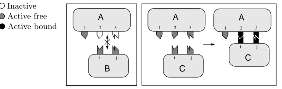
The above conditions, however, are not enough. A domain of a molecule can be either active or inactive. An inactive domain can never bind, not even when a complementary domain with the right orientation is close to it. In order to acti-vate a domain, a molecule needs to be involved in some reaction, for example in a phosphorylation (binding of a phosphate group to the protein). Active domains may further be free or bound. So domains are classified depending on three pos-sible states: active bound, active free, and inactive. Figure 2 shows a schematic

A B 1 2 3 i j A 1 2 3 A 1 2 3 i j C C i j Active bound Active free Inactive

Figure 2: Interfaces, sites, and states

representation. Biological entities (named A, B, and C in the picture) possess an

interface (the rounded box with colored hooks). Each interface has n >0 sites (the hooks sticking out the rounded box), and each of them can be in one out of three states (the color of the hook) as said above. A site is an indivisible structure that can only join to a complementary site. In the scenario drawn in Figure 2, A cannot bind to B. In fact, sites2 and i are complementary, just as 3 and j, but 2 and 3 are both inactive. On the contrary, A and C can bind together: sites i and2, and j and 3 are pairwise complementary, and all of them are active free.

An interesting point is relative to the possibility of dynamically changing the number of sites available on a given interface or their states. In general, might be necessary to be able to add sites (see the running example in Sect. 5).

Finally, an important aspect of biological entities is their shape. Indeed two molecules can interact if they can get in touch accommodating their shapes. Con-sider for instance Figure 3(a) where entities A and B can interact through sites 1 and 2. The interaction can change the involved electrostatic forces. It can modify the shape of the new complex, and eventually make site 3 available for interaction (Figure 3(b)).

Concluding, an interaction site can be inactive either because a chemical re-action is needed to activate it, or because it is hidden by the three-dimensional structure (shape) of the hosting component.

(9)

A 2 3 B 1 _B 1 A 3 ₂ (a) (b) Figure 3: Shapes 3.2 Compartments

The same biochemical reaction in a different spatial context may have different outcomes. For instance, the bacterium Escherichia coli (E.coli) lives in the lower intestines of mammals performing useful functions involving the digestion of its host. If E.coli escapes the intestinal gap through a perforation (e.g. a hole from an ulcer), and enters the abdomen, it can cause an infection called ‘peritonitis’, fatal without immediate treatment. This example shows that it is important for a modeling language to allow the modeler to easily deal with compartments and with their possible modifications. These latest phenomena can be classified as endocytosis, exocytosis, break and merge.

• Endocytosis and exocytosis. Endocytosis consists in absorbing substances from the external environment. Endocytosis can be further distinguished in pinocytosis (assumption of liquids: no particle is absorbed except those contained in the liquid), phagocytosis (absorption of another component of comparable size), and generalized endocytosis (absorption of an arbitrary number of smaller components). Exocytosis is the opposite of endocytosis, i.e. the expulsion of sub-components.

• Break and merge. Break is used to model phenomena that imply a change in the boundary of a component. We consider lysis, mitosis and meiosis. Lysis is the disintegration of a cell following a damage of its plasma membrane. It makes free the biological material inside the membrane. Mitosis, typical of viruses, consists in the exact duplication of the cell. Meiosis, typical of reproductive cells, is the separation of the cell and of the contained genetic material and yields two new cells. The phenomenon opposite to break is called merge.

Figure 4 summarizes the four primitives which we define following the inspiration gained by the above observations. We call those primitives EXO, ENDO, BREAK and MERGE, respectively.

Finally, when dealing with the interaction of molecules within cells, the com-partments might be thought of as the cellular comcom-partments or the molecules. For

(10)

EXO

ENDO

MERGE BREAK

Figure 4: Compartment primitives

example, one important event that occurs within cells is the movement of small molecules across compartment membranes. Hence, we also consider the opera-tions representing uniport (the movement of one molecule across a membrane),

symport (the simultaneous movement of two molecules across a membrane in the

same direction) and antiport (the simultaneous movement of two molecules across a membrane in opposite directions).

3.3 Further aspects

We now briefly sketch a set of interesting features of biomolecular processes which are independent on the concept of biochemical interactions and compartment and hence have not been presented yet. More details about the representability of these features in process calculi will be given later, when commenting on the various approaches used to face, respectively: reversibility; handling of quantitative infor-mation; and equivalence relations.

Reversibility

In nature many reactions are reversible. Reversibility is primarily governed by the kind of bonds that one wants to destroy and the available energy. Consider for instance the case when two proteins A and B are competing to bind to C (Figure 5). The system may evolve in three distinct ways. The case when both A and B bind to C gives raise to an unstable complex: sooner or later A or B will leave it. If A and B are, respectively, the activator and the inhibitor of C, and the global system is a molecular switch, then it is fundamental to be able to reverse the unstable complex. Reversibility is a basic regulation mechanism that, for example, prevents dead-locks. It can be specified in process calculi either in an explicit way, by means of

(11)

B A B A C B A C B A C C

Figure 5: Reversible complexation

Quantitative information

The ability of reasoning about quantitative information plays a crucial role in biomolecular processes. For example, in order to correctly describe a reaction it is necessary to know the exact quantity of reactants involved, the affinity of the sites available for bonds, and the amount of energy which can be used. Represent-ing and handlRepresent-ing quantitative parameters typically results in both a formal and an implementation overhead. Nonetheless, this is a crucial point for building useful models of biological systems.

Equivalence

Two programs are usually considered equivalent in computer science if they exhibit the same behavior w.r.t. some chosen notion of observation. Different definitions of observation lead to distinct equivalence relations. The desired property is then that two equivalent components can be safely exchanged within a system without altering its overall behavior (if this property holds the equivalence turns out to be a congruence). An analogous situation is found in biology. Up to a certain equiv-alence relation, eukaryote cells and prokaryote cells might be seen as belonging to the same class of organisms. In order to relate distinct kinds of lymphocytes it would be surely necessary a finer grained notion of equivalence.

As far as systems described by terms of process calculi are concerned, equiv-alence relations are fundamental tools for both analysis and verification. It could well be the case that the techniques developed in concurrency theory may help in the formalization and the understanding of biomolecular relations. Further investi-gation is needed to relate the biological notions of relations (e.g., homology) and the computer science behavioral equivalences.

(12)

4 Process calculi abstraction principle

Abstraction is the mechanism of withdrawing information content from a

knowl-edge domain in order to focus on the facts that seem most relevant for a particular purpose. Computer science deeply leans upon abstraction. For instance, comput-ers work by simply checking presence or absence of electronic signals at physical level. With a similar capability it becomes even difficult to do simple operations like

var := var + 3 (1 )

that increments the value of a variable var . Hence suitable abstractions are needed to make it easy give instructions to computers ans abstractions can be arranged hi-erarchically (firmware, assembler, operating systems, high-level programming lan-guages, etc.). For instance, the low level steps required for(1 ) are quite complex: load the value of var into a registry, convert3 to binary representation, decompose calculation into assembly instructions and so on. Moreover, the resulting program heavily depends on the underlying hardware architecture. High level languages (e.g. C++, Java ) allow to forget (i.e. abstract away) implementation details and to focus on the programming activity. This approach boosted computer science over the last 40 year. The idea is to exploit the same principle in systems biology.

Biology Process calculi

Entity Process

Interaction capability Channel Interaction Communication Modification/evolution State change

Table 1: Process calculi abstraction for systems biology

Assume to know the basic mechanisms that ‘drive’ life. If we are able to design a low level language that embeds the above mechanisms, we can explore biolog-ical hierarchies through compilation and then use living matter as our hardware infrastructure. In a similar vision, language theory is a conceptual formal tool that enables biologists to reassemble fragmented knowledge into a whole biolog-ical system via computational thinking. Process calculi play the role of low level languages, because their theory coincides at some extent with an abstraction of molecular interactions. Table 1 gives a concise picture of the map between biol-ogy and process calculi. A biological entity (e.g., a protein) is seen as a compu-tation unit, a process, with interaction capabilities abstracted as channel names. Entities interact/react through complementary capabilities as processes communi-cate/synchronize on complementary actions. The change of a state after a commu-nication represents the modification/evolution of molecules after a reaction.

The abstraction in Table 1 has four main properties [65]: (i) it captures an essential part of the phenomenon; (ii) it is computable, or better, it is executable, allowing computer aided analysis; (iii) it offers a formal framework to reason; (iv) it can be extended. In the rest of the paper we will show the main process calculi proposed for representing biological systems, and we will show how each one focuses on a particular extension of the abstraction principles in Table 1.

(13)

Virus Various Inactive Lymphocytes Lymphocyte Active Macrophage Lysis Mating Phagocytosis

Figure 6: Lymphocyte T helper activation

5 Running Example

This section introduces the running example that will be used to present and com-pare the considered calculi in the biology applicative domain. The example comes from the biology of the immune system, and it is relative to the activation of the

lymphocyte T helper.

The example has been chosen taking in mind two essential factors: (i) the example has to be sufficiently complex to be an interesting case study for represen-tation issues; (ii) it must be abstract enough to allow independence from irrelevant biological details. These features ensure that a short description of the phenomenon can make it easily accessible to readers without any specific background in biology. Lymphocytes T are eukaryote cells belonging to our immune system. There are three different sorts of lymphocytes T: lymphocytes T helper, lymphocytes T sup-pressor, and lymphocytes T cytotoxic. The lymphocytes of the first two classes are the main controllers of the immune system. Lymphocytes T cytotoxic work against foreign eukaryote cells and against cells of the body which have been infected by a virus.

Lymphocytes are normally inactive, and start their activity only after being triggered by special events. Each class of lymphocytes may be activated in many ways. We will focus on the activation of lymphocytes T helper performed by macrophages.

Macrophages are cells belonging to our immune system. They can engulf a virus by endocytosis, and, when this happens, the virus is degraded into fragments and a molecule (antigen) is displayed on the surface of the macrophage. The

(14)

anti-gen may be recognized by a lymphocyte T helper, and this activates the mecha-nisms of the immune reply, like, e.g., the duplication of the lymphocyte. Notice that the phenomenon includes the following relevant ingredients:

• pattern recognition, that allows the macrophage to distinguish malicious antigens and to activate the appropriate T cell;

• membrane interactions, that allow the macrophage to engulf viruses and to express antigens;

• internal pathways, that lead to the digestion of the engulfed viruses.

Figure 6 gives an abstract representation of the phenomenon described above. Viruses are modeled as entities with inactive sites which represent the viral anti-gens, i.e., the molecules characterizing the viruses. The process starts with the phagocytosis (ENDO) of the virus by the macrophage. The virus is then decom-posed (BREAK), and eventually viral antigens are moved to the surface of the macrophage. So the macrophage acquires some active sites from the virus, and can wait for a lymphocyte with a complementary site. When the appropriate lym-phocyte T helper binds to the macrophage, it becomes active and starts playing its role in the immune reply. Observe that lymphocytes have active sites even before binding to a macrophage. Indeed, even if in this state lymphocytes are inactive, as all in the immune reply, no binding would be possible without active sites.

6 Calculi for biology

In this section we survey the main calculi for biology which have been proposed in the literature. For each calculus, we first consider the representation of the com-partments, and then we refine the model at the biochemical level. We will exploit short portions of code for the activation of lymphocytes T helper. Finally, for each calculus we will comment on the expressivity w.r.t. the biological requirements proposed in Sect. 3, and on the availability of software.

6.1 Biochemical stochastic π-calculus

The biochemical stochastic π-calculus [66, 62] represents biochemical systems of interacting molecules as mobile communicating processes of the π-calculus [48, 69]. Public channel names and co-names represent complementary sites and cellular compartments are rendered by the appropriate use of restrictions on chan-nels. Molecular interaction is modeled as communication, and the stochastic ex-tension of the π-calculus [60] is adopted to provide quantitative descriptions of systems.

6.1.1 Syntax and Semantics

The π-calculus is a name-passing process calculus where names are synonyms of both data and channels. Its biochemical stochastic extension represents molecules as computational processes. A molecular complex is a system of processes sharing a private name which is unknown outside the complex. In this way, a molecule

(15)

which is external to the complex can by no means have access to the complex. The scope of the private name represents the boundary of the complex. Movements be-tween complexes and formations of new complexes are represented by transmitting private names (the so-called name extrusions).

The biochemical stochastic π-calculus represents interfaces by means of com-munication channels. Components interact by communicating on complementary sites, and interfaces may be possibly modified as a result of the communication.

6.1.2 Example

System specification

SYS::= MACROPHAGE|VIRUS|TCELL1|TCELL2 MACROPHAGE::=(νMemM)(TlrhMemMi. MemM(a).!ahstri)

VIRUS::=(νMemV)(Tlr(y).yhAnt1i)

System evolution

MACROPHAGE|VIRUS→

(νMemM) ( MemM(a).!ahstri |(νMemV)(MemMhAnt1i))→

(νMemM)(!Ant1hstri)

Figure 7: Phagocytosis-Digestion-Presentation in π-calculus

Compartments. Figure 7 reports the a code fragment that encodes the anti-gen presentation phase. The global system SYS is given by the parallel com-position of four processes: VIRUS, MACROPHAGE,TCELL1, and TCELL2. Figure 7 only presents the specifications of the first two elements. Here we just sketch the intuition of the behavior of the sub-system given byMACROPHAGE|

VIRUS. The restriction on top of each component stands for its enclosing mem-brane. The macrophage phagocytes the virus by means of a communication on the public channel Tlr. Operationally, this communication involves the output action

TlrhMemMi and its complementary input actionTlr(y), and its effect is twofold: (i) the restricted name MemM undergoes a scope extrusion and becomes a pri-vate resource of both MACROPHAGE and VIRUS (thus modeling the engulf-ment of the virus); (ii) the name yinVIRUS is renamed intoMemM(modeling the adaption of the internal machinery of the macrophage to start the lysis). The subsequent communication over the channel MemMis such that the datumAnt1

is transmitted to MACROPHAGE, which can make it available to lymphocytes T (TCELL1, TCELL2) by means of the latest action !Ant1hstri. The operator bang, !, allows to model infinite behaviors. In particular, !Ant1hstri behaves as

Ant1hstri. (!Ant1hstri), and thereforeMACROPHAGEcan activate many TCells expressingAnt1.

Biochemical interactions. Figure 8 shows the implementation of the activation of the appropriate lymphocyte T helper. Assume that the antigen presentation phase

(16)

already occurred, and hence that the macrophage is ready to communicate on chan-nelAnt1with whichever lymphocyte can execute a complementary action on the same channel. In the evolution drawn in Figure 8 this lymphocyte is TCELL1

which, after the synchronization on Ant1, can start its activities. Notice that the active form of the macrophage,MACROPHAGE’, can activate another TCell be-cause of the bang operator.

SYS::=MACROPHAGE’|TCELL1|TCELL2 MACROPHAGE’::=(νMemM) (!Ant1hstri)

TCELL1::=(νMemT1)(Ant1(x).ACTIVITIES) TCELL2::=(νMemT2)(Ant2(x).ACTIVITIES)

System evolution

SYS→

MACROPHAGE’|(νMemT1)(ACTIVITIES)|(νMemT2)(Ant2(x).ACTIVITIES)

Figure 8:TCELLactivation in π-calculus

6.1.3 Comments

The biochemical stochastic π-calculus represents biochemical interactions as com-munications, yielding models of biological pathways which are both detailed and concise. In the biochemical stochastic π-calculus there is no explicit concept of compartments. To represent the operations on compartments (EXO, ENDO, BREAK and MERGE), the non-intuitive concepts of restriction and name passing must be used.

There exist implementations of the biochemical stochastic π-calculus that make real in silico experiments possible. Two examples of simulation tools for biochem-ical stochastic π-calculus are BioSpi [72] and SPiM [57], both based on the Gille-spie’s algorithm [25]. Several complex models of real biochemical systems have been implemented and simulated by using these tools. Notably, the simulation of extra-vasation in multiple sclerosis reported in [45] showed to have a sort of predictive flavor: an unexpected behavior of leukocytes has been guessed by the results of in silico simulations, and proved a posteriori in lab experiments. Also, a whole virtual cell (VICE), with a basic prokaryote-like genome (about 180 dif-ferent genes) is developed with interesting results: for instance, the distribution of metabolites along the glycolytic pathway of VICE significantly matches with those of real organisms [14].

To overcome the intrinsic difficult in π-calculus, due to its minimal sintax, some eorts are devoted to design higher-level languages that provides direct support for the concepts needed in modeling biological systems, as e.g. [21] that leads to a complex model of gene regulation [44].

(17)

6.2 BioAmbients

BioAmbients [64] focuses on compartments: the location of molecules within

spe-cific compartments is considered a key issue for regulatory mechanisms in biolog-ical systems. Biomolecular systems are organized in a hierarchbiolog-ical and modular way: a molecule can perform its task if and only if it is in the right compartment.

Ambients are the boundaries of a set of processes which can communicate with each other. Ambients can be nested and hence they are organized hierarchically.

As for the π-calculus, we do not provide a full description of the calculus. We rather focus on a few main features which are useful for our presentation. The reader is referred to [64] for full details.

Depending on the relative locations of the interacting processes, three kinds of communication are defined in BioAmbients:

• local, namely between two processes in the same ambient, • s2s, namely between two processes located in sibling ambients,

• p2c / c2p,namely between processes located in ambients with a parent-child relation.

As far as the interpretation of movements is concerned, three pairs of primitives are defined as process actions:

• enter n / accept n, for entering an ambient and accepting the entrance, respectively,

• exit n / expel n, for exiting from a containing ambient and expelling a con-tained ambient, respectively,

• merge+ n / merge- n, for merging two ambients together. 6.2.2 Example

Compartments. Figure 9 shows a possible specification of the digestion of the virus by the macrophage. The two processesInfectandDigestabstract the infec-tion capability of the virus and the digesinfec-tion capability of the macrophage, respec-tively. Virus and macrophage synchronize on channeltlr, and the virus enters the macrophage by anenter / acceptpair. Then the virus sends its antigen on channel

tlr, and eventually the macrophage makes the antigen available to lymphocytes T helper.

Biochemical interactions. BioAmbients uses communication channels to imple-ment ‘interfaces’ of biological entities (as the biochemical stochastic π-calculus). The BioAmbients implementation of the activation of the lymphocyte T helper by a macrophage is reported in Figure 10. Each lymphocyte reacts to a specific antigen and begins its task by means of a communication on a dedicated channel. After the right lymphocyte has been activated, the macrophage can activate other TCells, because of the bang operator!.

(18)

Digest Infect Virus enter tlr. c2p trl!{ant1} Digest Infect Digest Infect Macrophage

accept tlr. p2c trl?{y}. ! s2s y!{str}

Macrophage Virus Macrophage Virus c2p trl!{ant1} p2c trl?{y}. ! s2s y!{str} ! s2s ant1!{str}

Figure 9: Phagocytosis-Digestion-Presentation in BioAmbients

Digest s2s ant1!{str} Macrophage Digest s2s ant1!{str} Macrophage TCell1 Active TCell2 s2s ant2?{m}.Active TCell1 TCell2 s2s ant2?{m}.Active Active TCell1 s2s ant1?{m}.Active TCell2 s2s ant2?{m}.Active TCell1 s2s ant1?{m}.Active TCell2 s2s ant2?{m}.Active Macrophage Macrophage ! s2s ant1!{str} ! s2s ant1!{str} Digest Digest

(19)

6.2.3 Comments

BioAmbients models biochemical interactions as communications on channels. It extends biochemical stochastic π-calculus communications with three kind of communications: interactions can occur between entities in the same compartment (local communication), between actions lying in ambients within the same ambi-ent (s2s communication), and between father-child ambiambi-ents (c2p/p2c communi-cation). BioAmbients is the first process calculus for modeling biological systems in which an explicit and intuitive notion of compartments is considered. It is easy to model in BioAmbients operations as EXO, ENDO and MERGE. BioAmbients has no primitive to represent the splitting of environments (BREAK), and it is not straightforward to model, e.g., mitosis. Other operations that can be easily mod-eled are complex formation and transport of small molecules across compartments. Hence, BioAmbients may represent, in this respect, an improvement compared to biochemical stochastic π-calculus: many biological phenomena are represented much more easily in BioAmbients than in π-calculus.

A stochastic extension of the language has been defined, and a simulator is im-plemented as part of the BioSpi project [72] based on Gillespie’s algorithm [25]. Control Flow Analysis, a static analysis technique that allows to analyze the de-scription of the system to discover dynamic properties, is adapted to BioAmbi-ents [50].

6.3 Brane Calculus and Projective Brane Calculus

Brane calculus [9, 10] is centered on membranes, and it is based on the observation

that membranes are not just containers, but also active entities that take care of coordinating specific activities. Membranes can be highly dynamic: for example, they can shift or merge. Molecules can communicate using their membranes, and indeed large proteins are embedded in membranes which act like channels.

The main feature of Brane calculus is that membranes are considered active el-ements and hence the whole computation happens on membranes. In Brane calcu-lus membranes can move, merge, split, enter into and exit from other membranes. Some constraints need to be satisfied when applying these operations. The most important one is that transformations need to be continuous (e.g. a membrane, except the case it represents a small molecule, cannot simply pass across another membrane). Another constraint is that the orientation of membranes need to be preserved, so merging of membranes cannot occur arbitrarily (e.g. membranes with a different orientation cannot merge).

A system is represented in Brane calculus as a set of nested membranes, and a membrane as a set of actions; actions carry out the mentioned membrane trans-formations. The Brane calculus primitives are inspired to membrane properties. Because of the constraints on membrane operations, Brane calculus primitives are more restrictive than those we presented in Sect. 3.2. The primitives related to movement to and from membranes are classified in two main groups, one for cytosis-like and the other for mitosis-like phenomena.

(20)

• Endocytosis, corresponding to the ENDO operation, is considered an un-controllable process. Interesting interactions are usually more un-controllable, therefore two finer primitives are defined: phagocytosis (phago), for en-gulfing one external membrane, and pinocytosis (pino), for engulfing zero external membranes. Exocytosis (exo), which corresponds to the EXO op-eration, represents the expulsion of an internal membrane.

• Mitosis, corresponding to the BREAK operation, is also considered an un-controllable process, because it can split a membrane at an arbitrary place. Hence, two finer primitives are defined: budding (bud), for splitting off one internal membrane, and dripping (drip), for splitting off zero internal mem-branes. Mating (mate), which corresponds to the MERGE operation, repre-sents the controlled merging of two membranes.

For each action, a corresponding co-action is defined. Hence, as in BioAmbients, coordination between interacting components is always required. Communication can be on-membrane or cross-membrane, and they are associated with distinct pairs of primitives.

• On-Membrane. The primitivesp2pn/p2p⊥n are for on-membrane

commu-nications only.

• Cross-Membrane. The primitives s2sn /s2s⊥n, p2cn /p2c⊥n, andc2pn / c2p⊥

n are for communications between processes in distinct membranes and

follow a BioAmbients-like style.

Projective brane calculus. This calculus, which has been introduced in [18], is a refinement of Brane calculus. Its authors observe that in real life biological membrane actions are directed; therefore they refine brane calculus by replacing actions with directed actions, so that interaction capabilities are specified as facing inwards or outwards. This refinement results in an abstraction which is closer to biological settings than the original language.

6.3.2 Example

Compartments. Figure 11 reports a specification of the running example in Brane calculus. The operator◦ stands for parallel composition. The rounded parenthe-ses (| |) enclose the genetic content of the membrane, which is represented by a sequence of actions to the left of the symbol(|.

During the synchronization overphago, the virus communicates its antigen to the macrophage on the channel trl. Then the macrophage presents the antigen to the environment. As mentioned in Sect. 6.2, in real life a virus does not actually send its antigen to a macrophage.

Biochemical interactions. Figure 12 shows the Brane calculus code for the ac-tivation of the appropriate lymphocyte.

(21)

SYS::= VIRUS◦ MACRO ◦ TCELL1 ◦ TCELL2

VIRUS::=phagotrl.c2pn(ant1).INFECT(|CAPSID|)

MACRO::=phago⊥

trl(DIGEST).c2p⊥n(a).s2sa(str)(|CYTOSOL|)

DIGEST::=c2p⊥

n(a).c2pn(a).DIGEST

System evolution MACRO◦ VIRUS →

c2p⊥

c2p⊥

Figure 11: Phagocytosis-Digestion-Presentation in Brane calculus

SYS := MACRO◦ TCELL1 ◦ TCELL2

MACRO::=s2sant1(str).PHAGO(|CYTOSOL|)

TCELL1::=s2s⊥

ant1(x).ACTIVITIES1(|CYTOSOL|)

TCELL2::=s2s⊥

ant2(x).ACTIVITIES1(|CYTOSOL|)

System evolution

SYS→ PHAGO(|CYTOSOL|) ◦ ACTIVITIES1(|CYTOSOL|) ◦ TCELL2

Figure 12:TCELLactivation in Brane calculus

6.3.3 Comments

In Brane calculus everything is interpreted as a membrane, which means that membrane-bound cellular compartments (e.g. cells and organelles) and molecular compart-ments (e.g. proteins) are modeled in the same way. The language does not take the internal structure of membrane-bound compartments into account, therefore it is not easy to describe biochemical events that are not directly related to cellular membranes, such as protein activation, phosphorylation, etc.

Brane calculus is inspired by BioAmbients, but it gives membranes an active role. The notion of membrane as an active entity and not just a simple container is surely relevant. In addition, Brane calculus primitives are realistic and provide a simple and intuitive way to model the most important membrane operations. Being Brane calculus primarily concerned on membrane interactions, it is possible (and also relatively easy) to model all kinds of operations involving compartments (EXO, ENDO, MERGE, BREAK) and also movements of small molecules across membranes. No software tool is available for this calculus.

(22)

6.4 CCS-R

CCS-R [15] explicitly deals with the issue of reversibility: most biochemical re-actions are, indeed, reversible. Based on this observation, CCS-R is a CCS-like process algebra [47] with the peculiarity that reversibility is embedded in the syn-tax. No handling of energy and types of bonds is considered, although they are the driving forces of biomolecular reversibility.

CCS-R is a ‘decoration’ of CCS with the concept of reversibility. This feature of the language is relevant when considering biochemical scenarios. Regarding the description of compartments, instead, CCS-R may be considered the same as CCS: a process algebra that describes the interactions between processes in terms of binary synchronized communications and does not use either value or name-passing. In CCS-R it is not possible either to send a name on a channel or to dynamically change the scope of a restricted name. For this reason, compartments and information flows between processes cannot be represented.

CCS-R generalizes CCS duality between names and co-names to a binary com-plementation relationC between binding sites: the two sites x and x0 _{can connect}

together only if xCx0_{. Moreover, based on the observation that some protein}

inter-actions require a concurrent connection to different sites, the standard CCS syntax is extended to allow processes likeC= (l’₁ |l’₂|l’₃).0to represent the fact that the sites of C must be activated simultaneously. Apart from these differences, CCS-R is the same as CCS. In particular, for what concerns our example, the system specifications in the two languages are identical.

6.4.2 Example

SYS::=(νTlr)(νAnt1)(νAnt2)(VIRUS|MACROPHAGE|TCELL1|TCELL2) VIRUS::=Tlr.Ant1.INACT

MACROPHAGE::= Tlr.DIGEST

System evolution

SYS→(νTlr)(νAnt1)(νAnt2)(Ant1.INACT|DIGEST|TCELL1|TCELL2)

Figure 13: Phagocytosis-Digestion-Presentation in CCS-R

Compartments. As previously mentioned, compartments cannot be represented in CCS-R, and the information flow from the virus to the macrophage cannot be faithfully rendered. It is still possible, though, to specify the antigen presentation phase as a pathway activation. This kind of coding is used in the specification

(23)

of the running example in CCS-R, shown in Figure 13. Notice that, in order to overcome the fact that the position of restrictions cannot change at run-time, the relevant resources have to be declared as private channels of the top-level process

SYS.

SYS::=(νTlr)(νAnt1)(νAnt2)(VIRUS|MACROPHAGE|TCELL1|TCELL2) MACROPHAGE::= DIGEST VIRUS::=Ant1.INACT TCELL1::=Ant1.ACTIVITIES1 TCELL2::=Ant2.ACTIVITIES2 System evolution SYS→

(νTlr)(νAnt1)(νAnt2) (INACT|DIGEST|ACTIVITIES1|Ant2.ACTIVITIES2)

Figure 14:TCELLactivation in CCS-R

Biochemical interactions. CCS-R is particularly suitable to represent biochem-ical interactions. However, since it does not use a name-passing discipline, it is impossible to directly render the information flow between processes and its sub-sequent changing of the possible evolution of the communicating partners. With respect to the previous code fragments, let us consider the antigen passing from the virus to the macrophage and, finally, to the rightTCELL: in the CCS-R specifica-tion for lymphocyte activaspecifica-tion (Figure 14), the virus (rather than the macrophage) is responsible for activating the rightTCELL.

6.4.3 Comments

CCS-R, being based on CCS, allows to represent biochemical pathways as a cas-cade of synchronized interactions. CCS-R does not allow name passing or a di-rect representation of biological bounds, therefore modeling compartment is not directly supported.

CCS-R has primarily been developed to implement reversibility in a process calculus for biology. The authors of CCS-R think of reversibility as the ability to backtrack from a reaction and claim that this is a common phenomenon in nature. This is true, however, only if the energy of the system is not considered. Indeed the second principle of thermodynamics states that going back exactly to the orig-inal system is not possible. This principle could become crucial if reversibility was investigated together with a quantitative analysis of the global energy of the biological system. No software tool is available for this calculus.

(24)

6.5 PEPA

Performance Evaluation Process Algebra (PEPA) [31] is a formal language for

de-scribing Markov processes. PEPA was introduced as a tool for performance analy-sis of large computer and communication systems to study in the same framework quantitative properties as throughput, utilization and response time and qualita-tive properties as deadlock freedom. With the advent of the systems biology era, the abstraction facilities of PEPA was exploited in biochemical signaling pathways analysis and simulation [8].

PEPA differs from the previous calculi because it adopts multiway synchronization on shared name in the style of the Communicating Sequential Processes (CSP) [33] rather than complementarity (as CCS and π-calculus). The cooperation operator

BC

L requires the “co-operands” to join for activities specified in the cooperation

set L. Consider a simple biochemical reaction r1 where two protein Prot1 and

Prot2 interact with a rate k₁and form a protein Prot3 . The system is specified by the following:

Prot1H ::= (r1, k1).Prot1L

Prot2H ::= (r1, k1).Prot2L

Prot3L::= (r1, >).Prot3H

Sys::=Prot1H _{r1}BCProt2H _{r1}BCProt3L

The subscript H and L stay for high and low level of protein. The three protein can synchronize on activity r1 enabling the transition:

Sys −−−−→ Prot1(r1,k1) L_{r1}BCProt2L_{r1}BCProt3H

where low levels of Prot1 and Prot2 are present and an high level of Prot3 is reached. The multi-way synchronization underlying PEPA allows the three pro-cesses to advance in one step. This is the main difference of PEPA w.r.t. CCS/π-calculus style of interaction.

6.5.2 Example

Compartments. PEPA cannot represent directly compartments or inderectly by means of scope extrusion. The information flow from the virus to the macrophage on Trl cannot be faithfully represented, but, by specifying the antigen presenta-tion phase as a biochemical interacpresenta-tion, it is still possible . The approach is the same used in CCS-R, and Figure 15 shows the related PEPA code. Macrophage

MACROP synchronize with VIRUS on activity Tlr enabling Ant1presentation with a rate k.

Biochemical interactions. PEPA represent biochemical interactions as cooper-ation, meaning that processes jointly perform actions of the same type. However, PEPA has not name-passing features, and therefore PEPA does not allow to directly represent information flow and subsequent changing of the interaction capabilities. Figure 16 sketches PEPA code for TCell activation. The virus (rather than the

(25)

SYS::=VIRUS BC

{T lr} MACROP

VIRUS::= (Tlr,k) . (Ant1,kA1) . INACT

MACROP::= (Tlr,k) . DIGEST

System evolution

SYS−−−−→(Tlr,k) (Ant1,kA1) . INACT _{{T lr}}BC DIGEST

Figure 15: Phagocytosis-Digestion-Presentation in PEPA

System specification SYS::= VIRUS’ BC {Ant1,Ant2} MACROP’ BC {Ant1,Ant2} TCELL1 BC {Ant1,Ant2} TCELL2 MACROP’::= DIGEST VIRUS’::=(Ant1,kA1) . INACT TCELL1::=(Ant1,kA1) . ACTIVITIES1 TCELL2::=(Ant2,kA2) . ACTIVITIES2 System evolution SYS−−−−−−→(Ant1,kA1) INACT BC {Ant1,Ant2} MACROP’ BC {Ant1,Ant2} ACTIVITIES1 BC {Ant1,Ant2} TCELL2

Figure 16:TCELLactivation in PEPA

macrophage) synchronize with the TCell with the right antigene. Notice that Ant2 is in the cooperation set{Ant1 , Ant2 } because otherwise TCELL2can proceed without recognizing the right antigene.

6.5.3 Comments

PEPA was introduced as a tool for performance analysis. Its application to systems biology allows to quantitatively model and analyze large pathway systems (e.g., [7]). However, PEPA lacks in expressivity of compartment primitives.

PEPA has two main characteristics that makes it very interesting, also for biol-ogy: (i) a large community supporting it [35] with a reach availability of software tools. For instance, the PEPA Workbench [26] allows to exploit Markov process analysis on PEPA specification. Moreover, external tools support PEPA. For in-stance, the PRISM model checker [32] accepts model descriptions in the PEPA formalism. (ii) PEPA is a language for describing Markov processes, and there-fore PEPA is developed with a strong mathematical background. This enables the

(26)

comparison and convergence of process calculi models and classical ODE mod-elling [5, 6].

6.6 Beta-binders

Beta-binders [61] is a bio-inspired process calculus that interprets biological

enti-ties as an internal “process unit” and an “interface” exposed to the external environ-ment. By introducing the concept of affinity, the interaction approach extends the CCS notion of complementarity between action and coation. Beta-binders com-munication models is inspired by enzyme theory [43], where interactions between not perfectly matching components are allowed.

In Beta-binders, π-calculus processes are encapsulated into boxes with interaction capabilities. The π-calculus syntax is enriched by operations for manipulating in-teraction capabilities, that are represented by specialized binders. Any biological entityEis represent as a box BE

PE

x1: ∆1 . . . xn: ∆n

Types∆iexpress the interaction capabilities of the box. The parallel composition

of boxes, called bio-process, models a system of interaction biological entities. Two boxes can interact if they have complementary types up to a certain

user-defined notion (see [59] for an example). Here we adopt the original interpretation,

where types are sets of names and two types∆1and∆2are affine if∆1∩ ∆2 6= ∅.

The dynamic behavior of entity box BEis specified through the internal pi-process

PE. A pi-process is a π-calculus process, extended for manipulating the interface

of a box. For instance, hide and unhide actions make respectively invisible and visible an interaction site, allowing the direct representation of dephosphorilation and phosphorilation. Finally, two boxes can bring together (join) and one box in two can divide in two (split).

6.6.2 Example

Compartments. Figure 17 reports the Beta-binders fragment that encodes the antigen presentation phase. The global systemSYSis given by the parallel compo-sition of four boxes representing theVIRUS, theMACROPHAGE, theTCELL1, and the TCELL2, respectively. Figure 17 only presents the specifications of the first two elements and we just sketch an explanation of the behavior of the sub-system given by the MACROPHAGEand theVIRUS. The macrophage phago-cytes the virus by means of a join operation. This results in a box whose inter-action capabilities are inherited fromMACROPHAGE, and whose body is essen-tially given by the parallel composition of the internal bodies of the original boxes PMACRO and PVIRUS. After that, virus and macrophage are in the same box, so

they can communicate, and the name Ant1 is transmitted toMACROPHAGE,

which can make it available to lymphocytes T (TCELL1,TCELL2) by means of the latest output actionAnt1hstri.

(27)

System specification SYS::= PMACRO x: {v1, v2, ...} PVIRUS y: {v1} PTCELL1 x: {Ant1} PTCELL2 x: {Ant2}

PM ACRO::= x(w).expose(z, {w}) . (!zhstri | PDIGEST)

PV IRU S ::= yhAnt1i. PINFECT

System evolution PMACRO x: {v1, v2, ...} PVIRUS y: {v1} → PMACRO | PVIRUS x: {v1, v2, ...} →→

!zhstri | PDIGEST | PINFECT

x: {v1, v2, ...} z: {Ant1}

Figure 17: Phagocytosis-Digestion-Presentation in Beta-binders

Biochemical interactions. Figure 18 shows the implementation of the activation of the appropriate lymphocyte T helper. We imagine that the antigen presentation phase already occurred, and hence the macrophage is ready to execute an inter-communication on channel with type is Ant1 with whichever lymphocyte can ex-ecute a complementary action on a channel with a compatible type. In the system of Figure 18 this lymphocyte isTCELL1which, after the interaction, can start its activities.

6.6.3 Comments

Beta-binders was specifically designed to model biological interactions. The main peculiarity of Beta-binders is the concept of affinity, which allows not perfectly matching components to interact. This is often the case in biology, where the in-teraction sites of proteins can be compatible even if not exactly complementary. Biochemical events that are not directly related to cellular membranes (e.g. pro-tein activations, phosphorylations, etc.) can be easily modeled by Beta-binders communications and operations on box interfaces.

Another interesting feature of Beta-binders is that operations such as fusion of membranes and splitting of one membrane into two submembranes, can be easily modeled by means of the appropriate join and split primitives. However, when dealing with compartments one main drawback of Beta-binders arises: nesting of boxes is not allowed, so it is not intuitive to model hierarchies of entities. In [28] an extension of Beta-binders with an explicit notion of compartments is introduced. This extension permits to represent static hierarchical structures and the movement of components across compartments.

(28)

System specification SYS::= PA MACRO x: {v1, v2, ...}z : {Ant1} PTCELL1 a: {Ant1} PTCELL2 a: {Ant2}

PA M ACRO::=! ahstri | PDIGEST

PT CELL1::= a(y).PACTIVITIES1

PT CELL2::= a(y).PACTIVITIES2

System evolution SYS→ PA MACRO x: {v1, v2, ...}z : {Ant1} PACTIVITIES1 a: {Ant1} PTCELL2 a: {Ant2}

Figure 18:TCELLactivation in Beta-binders

Finally, Beta-binders is equipped with a stochastic semantics [19] and the asso-ciated simulation environment [68] for the in-silico study of biochemical pathways.

6.7 κ-calculus

κ-calculus [16, 17] is a formal calculus of proteins interaction. It was conceived to represent complexation and decomplexation of proteins. The κ-calculus comes equipped with a very clear visual notation, and uses the concept of shared names to represents bonds.

The units of κ-calculus are proteins, and operators are meant to represent creation and division of protein complexes. Proteins are drawn as boxes with sites on their boundaries. A site can be either visible, hidden or bound. For instance

M2 M1s2 s3 s4 s1

represents two bounded molecules M1and M2on sites s2 and s3, respectively. Moreover, the sites1ofM1is hidden and the sites4is visible.

Besides the graphical representation, the κ-calculus provides a language in the style of process algebras. Expressions and boxes are given semantics by a set of basic reactions. Once the initial system has been specified and the basic reductions have been fixed, the behavior of the system is obtained by rewriting it after the reduction rules. This kind of reduction resembles pathway activation.

(29)

V V M ph in in a1 a1 ph M (a) System specification

r1: M(ph),V(in,a1)→(x)(M(phx),V(inx,a1))

System evolution

M(ph),V(in,a1) → r1

(x)(M(phx_),V(inx_,a1))

(b)

Figure 19: Phagocytosis-Digestion-Presentation in κ-calculus

Compartments. The calculus does not offer a natural support for the compart-ment layer. It is possible to represent the Phagocytosis-Digestion-Presentation ex-ample (see Figure 19(a)) as an activation pathway. The virus is rendered by the boxV, which has a visible sitein, used to enter a cell, and a hidden sitea1, which represents the antigen. The macrophage is represented by the boxM, which has a visible siteph, used to phagocytes a molecule.

Figure 19(b) shows the single reaction relevant to our running example. In this reaction rule, the superscript x inphxand inx means that the sites inand phare linked by the channel named x. This mechanism may resemble a possible handling of affinity between channels, although no quantitative measure is considered.

Biochemical interactions. Figure 20(a) shows the κ-calculus graphical repre-sentation of the activation of a lymphocyte T helper. After phagocytosis, the virus has a visible site a1, which represents its antigen: only the lymphocyte with the right site can bind it.

ph V ph M in a1 a2T2 T1 a1 V in a1 M a2T2 T1 a1

(a) Graphical representation System specification

r2: M(phx),V(inx,a1),T1(a1)→M(phx),V(inx,a1y),T1(a1y)

r3: M(phx),V(inx,a2),T2(a2)→M(phx),V(inx,a2y),T2(a2y)

System evolution

(x)(M(phx_),V(inx_,a1),T1(a1)) _{→ r} 2

(xy)(M(phx_),V(inx_,a1y_),T1(a1y₎₎

(b) Language representation

(30)

The graphical notation does not clearly represent the selection of the right lym-phocyte. This gap is filled by the formal model via the definition of the basic reac-tions. In particular, the system described in Figure 19(b) may be extended with the rules defined in Figure 20(b). By these rules, it is possible to infer the reduction shown in Figure 20(b).

6.7.3 Comments

The κ-calculus was designed to represent complexation and decomplexation of proteins, and therefore it does not allow to represent compartment primitives. We want to point out that the main goal of the authors of κ-calculus, i.e. to “provide a formalism that could be a suitable modeling language allowing direct descrip-tions of molecular events” [16], has been achieved in an effective way: the visual language is intuitive, and the formal one rather simple to use. Moreover, despite its simplicity, in [13], κ-calculus was shown to be expressive to translate Kohn Interaction Map [41], a diagrammatic formalism to represent networks containing multi-protein complexes, protein modifications, and enzymes.

7 Concluding remarks

The languages mentioned in this survey are quite different, and have been con-ceived for specifying entities at different levels of abstractions. As expected, none of them is ‘the perfect language’, which allows to model in an easy and correct way all kinds of biological operations. Each language, however, has some distinguish-ing features that make it particularly suitable for modeldistinguish-ing certain kinds of systems or operations.

We can classify the various calculi depending on whether they are adaptations or extensions of calculi introduced to specify distributed systems, or rather they have been directly defined to model biological systems. For convenience, we refer to the languages of the first family as to bottom-up calculi, and to the others as top-down languages.

Biochemical stochastic π-calculus, BioAmbients, PEPA and CCS-R are bottom-up calculi. They are based on languages used to describe distributed systems. The main advantages of bottom-up languages are that they can rely on well-assessed mathematical basis and they are well-known in the community of distributed sys-tems. The main drawback is that, since they were not meant to describe biological systems, they are often too abstract and not much intuitive.

Brane calculus, Beta-binders, and κ-calculus are top-down languages. Their authors made the opposite effort: they tried to identify the fundamental biological primitives and to represent them by the techniques and tools of concurrency theory. The advantages and drawbacks of top-down languages are opposite to those of bottom-up ones: these languages are usually more intuitive and more biologically correct but, since they are very recent, they lack theoretical works and few tools exist to allow them to be of practical use for validation/simulation purposes.

Some of the languages we have described permit an explicit representation of biological compartments: Brane calculus, BioAmbients and the Beta-binders extension with compartments. Therefore they can be more suitable to model phe-nomena at compartment level. Brane calculus is very interesting when the focus