Simulation of non-Markovian Processes in BlenX

(1)

Technical Report CoSBi 11/2008

Simulation of non-Markovian

Processes in BlenX

Davide Prandi

The Microsoft Research - University of Trento

Centre for Computational and Systems Biology

prandi@cosbi.eu

Corrado Priami

The Microsoft Research - University of Trento

Centre for Computational and Systems Biology

and

Dipartimento di Ingegneria e Scienza dell’Informazione, University of Trento, Italy

priami@cosbi.eu

Alessandro Romanel

The Microsoft Research - University of Trento

Centre for Computational and Systems Biology

and

Dipartimento di Ingegneria e Scienza dell’Informazione, University of Trento, Italy

romanel@cosbi.eu

(2)

Simulation of non-Markovian Processes in

BlenX

D. Prandi1, C. Priami1,2, and A. Romanel1,2

1

The Microsoft Research - University of Trento Centre for Computational and Systems Biology

2

Dipartimento di Ingegneria e Scienza dell’Informazione, University of Trento, Italy {prandi,priami,romanel}@cosbi.eu

Abstract. BlenXis a programming language designed for modeling entities that can change their behavior in response to external stimuli. The actual framework assumes interactions being exponentially distributed, i.e., an underlying Markov process is associated withBlenXprograms. In this paper we relax the Markov assumption by providing formal tools for managing non-Markovian processes withinBlenXand we show experimental evidences of the effectiveness of the approach.

1 Introduction

The strength of the interaction between two entities is usually thought as a two value logic, i.e., the interaction is possible or not. For instance, two CCS [1] processes interact iff they can perform complementary actions (input and output) on the same channel. The paradigm communication by compatibility [2], recently proposed with the process calculus Beta-binders [3], introduces a “fuzzy” vision, and lets interactions depend on a notion of compatibility of the involved parties. For instance, web-services use XML to describe provided services, and interactions are disciplined by a notion of compatibility between XML descriptions [4]. Also, biological interactions depend on structural and chemical complementarity of molecules, called affinity [5].

BlenX[6] is inspired to Beta-binders and it is designed for modeling entities that can change their behavior in response to external stimuli. A general entityE is depicted

as a box_B_E:

PE

b b b b

x1: ∆1 xn: ∆n BE

The program_P_Eis written in a process calculi style language, and allows to control the behavior of_B_E. In particular,_P_Eactivates proper replies to external signals caught by interaction sites_x_i: ∆i. Type∆idiscriminates among allowed and disallowed

inter-actions, mimicking interaction mechanisms based on compatibility.

TheBetaWBframework [7] is a computational tool that supports textual and vi-sual programming withBlenX. TheBetaWBcan be seen as an in-silico laboratory, where (in-silico) experiments can be designed (i.e., aBlenXprogram is written), simu-lated and analyzed. The quantitative component of the experiments is guaranteed by the stochastic capability ofBlenX, on the line of [8], where a continuous-time Markov pro-cess is taken as foundational quantitative model. The goal of this paper is to provide the

(3)

formal tools for managing non-Markovian processes withinBlenX. Our motivations are flexibility and abstraction. Assuming, as in Markov processes, that a random variable follows the negative exponential distribution with parameterλ, fixes expected value to λ−1_{and variance to}_λ−2_{, thus limiting the flexibility of the choice about variability in}

the stochastic model [9]. It is also the case that not all the quantitative data about the basic steps of a Markov process are available, and many steps are abstracted as a single step. Since the composition of negative exponential distributions is not exponentially distributed, general distributions are required to have better abstractions.

We start in Sect. 2 by providing a proved reduction semantics for a core subset of

BlenX, following the work in [10]. Proved reduction semantics is a rephrase of en-hanced operational semantics [11], a conceptual tool for describing the behavior of concurrent systems. In particular, the transitions of the system have rich labels that permit to recover information about the causal relation between transitions. A seminal work about causality and Beta-binders can be found in [12]. Here we introduce the no-tion of dependency in Sect. 2.1 to adapt the idea of causality toBlenX. Dependency is then employed in Sect. 2.2 to support enabling memory discipline [13], that is, the stochastic distribution of the execution of a transitionθ must be influenced by all the

transitions fired from the states whereθ was firstly enabled. We can therefore compute

the right stochastic distribution of aBlenXtransition. Sect. 3 proposes someBetaWB

simulations of non-Markovian processes. Sect. 4 concludes the paper with some final remarks.

2 Formal Treatment

In this section we provide a proved operational semantics in the style of [10] for a subset ofBlenX. In particular, for the sake of clarity, we do not consider events [7].

A binder has either the formβ(x, Γ ), or βh_{(x, Γ ), where the name x is the subject}

of the binder, andΓ ∈ T is the type of x. The domain T can be arbitrarily instanced

under the proviso that a symmetric compatibility relation is also defined, and that the predicateα( , ) : T × T → R+_{, which returns a value greater that}_{0 iff its argument}

types are compatible, is decidable. Example of domain T can be found in [2].

Intu-itively, a binderβ(x, Γ ) represents an active (potentially interacting) site of a box. If a

binder has been hidden to prevent interactions, it is represented asβh_{(x, Γ ).}

Metavari-ableβ+ranges over{β, βh_{}, and ∆, ∆}

1, . . . , Γ, Γ1, . . . range over site types. Interfaces

are generated by the following grammar:

I ::= β+(x, Γ )

|

β+_{(x, Γ ) I.}

An interface is well-formed when the subjects and the types of its binders are all dis-tinct. We will work only with well-formed interfaces. Auxiliary functionssub(I) and

typ(I) give the set of subjects and types of an interface I, respectively.

We assume two disjoint countable infinite sets: N of names ranged over by x, y, z, . . . and S of delays ranged over by τ1, τ2, τ3, . . .. Processes are defined by the following:

πβ

(4)

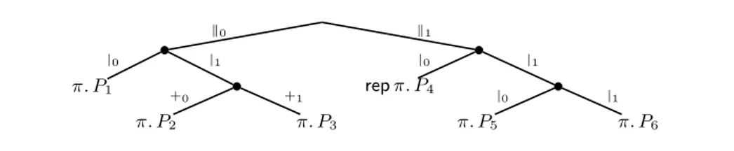
k0 π. P1 |0 |1 π. P2 +0 π. P3 +1 k1 repπ. P4 |0 |1 π. P5 |0 π. P6 |1

Fig. 1. The tree of the sequential processes within the boxes in the system (1).

Processnil, prefixes output x!v , input y?w , and delay τi, and operators of parallel

com-position | and choice + work as in π-calculus. Guarded replication rep π. P was

in-troduced in [14] and spawns a single copy ofP if prefix π is consumed. The prefixes hide(x), unhide(x), expose(x, Γ ), and ch(x, Γ ) manipulate the interface of a box and

will be further commented on when the semantics will be introduced. Finally, systems are defined by the following:

B ::=Nil

|

I

[

P

]

|

B k B .

The actual syntax ofBlenXdoes not univocally identify which actions are active in a given box. Consider, for instance, the following

I0[π. P1| (π. P2+ π. P3)

]

k I1[repπ. P4| (π. P5| π. P6)

]

(1)

A notion of address is needed to distinguish among the different instances of the prefix

π in (1). An address identifies a sequential component of a box B, namely, a process

with a prefix as a top-level operator. In particular, a b-addressϑb_{∈ {}_k

0,k1}∗,λbis the

empty one, identifies a box within a system, while a p-addressϑp _{∈ {}_|

0,|1,+0,+1}∗,

λp_{is the empty one, points to a specific sequential component of a process. Consider}

the abstract syntax tree of (1) in Fig. 1, built assuming parallel composition and choice as main operators. The leaves of the tree are the active processes. The label of the path from the root to a leaf is the address, e.g., processπ. P3has addressk0|1+1. Once a tree

of a system is fixed, an address uniquely identifies an active action.

Systems are decorated with addresses by a labeling functionT ( ). An auxiliary

operator. that distributes addresses among the sequential components is defined:

• ϑp_._nil₌_nil _{• ϑ}b_._Nil₌_Nil

• ϑp 1. (ϑ p 2π. P ) = ϑ p 1ϑ p 2π. (ϑ p 1. P ) • ϑ b . I

[

P

]

= ϑb I

[

P

]

• ϑp_{. (M} 1+ M2) = ϑp. M1+ ϑp. M2 • ϑb. (B1k B2) = ϑb. B1k ϑb. B2 • ϑp_{. (P} 1| P2) = ϑp. P1| ϑp. P2 • ϑp₁. rep ϑp₂π. P = rep ϑp₁ϑp₂π. P

The operator behaves as expected (see [10]), except for guarded replication repπ. P .

As it will become clear later, the address is not distributed overP in rep π. P , but the

task is delayed until the application of structural congruence. FunctionT ( ) inspects

a system and when a box k, a process parallel |, or a choice + is found, function .

T (P )

]

• T (rep π. P ) = rep π. P • T (B0k B1) =k0. T (B0) kk1. T (B1)

• T (P0| P1) = (|0. T (P0) | (|1. T (P1))

• T (M0+ M1) = (+0. T (M0)) + (+1. T (M1))

It is straightforward proving thatT () is a bijection between processes and boxes and

their labeled version, its inverse being the function that discards addresses. For this reason, in the following we will omit adjective labeled, and we will refer to processes and boxes leaving the context to discriminate.

The proved reduction semantics ofBlenXrequires the use of the structural congru-ence over both processes and boxes of Tab. 1. We overload the symbol≡ to denote

both congruences and let the context disambiguate the intended relation. The laws of structural congruence over processes are the typicalπ-calculus axioms except for the

rule of replication. In fact, the structural congruence rule for replication adds a parallel component after the prefixπ. Suppose to have a process rep τ1. τ2. The rule computes

the addresses ofτ1andτ2for each application of the structural congruence:

repτ1. τ2≡ τ1. (|0τ2| rep|1τ1. τ2) ≡ τ1. (|0τ2||1τ1. (|1|0τ2| rep|1|1τ1. τ2))

The meaning of the laws for boxes follows. First, the structural congruence of internal processes is lifted at the level of boxes. B-addresses are ignored. Second, the actual ordering of binders within an interface is irrelevant. Third, the subject of a binder can be refreshed under the proviso that name clashes in the internal process are avoided and that well-formedness of the interface is preserved. Finally, the monoidal axioms for the parallel composition of boxes are assumed.

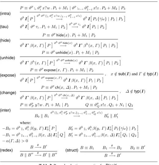
Tab.2 shows our proved reduction semantics forBlenX. Arrows carry labels holding the information needed to compute dependency relations. Labels, with metavariableθ,

have the form:

– ϑb_ϑp_π

β: a prefixπβwith p-addressϑpis consumed within boxϑb;

– ϑb_ϑp_h_|

iϑ

p

ix?w ,|1−iϑp_1−ix!z i: a communication within box ϑbis taking place; the

– ϑb_h_k

iϑb_iϑp_iy?w ,k1−iϑb_1−iϑp_1−ix!z i: a common context ϑb allows to reach

com-municating boxeskiϑb_i and k1−iϑb_1−i; p-addresses ϑ

p i and ϑ

p

1−i identify the

in-volved input and output prefixes, respectively.

The axiom(intra)defines communications between processes within the same box. The axiom reads as follows. If the internal process P is structurally equivalent to ϑp_|

iϑ

p

ix?w . P1+ M1 | ϑp|1−iϑ

p

1−ix!z . P2+ M2 | P3, then the box can perform a

reduction leading to a new box with unchanged interface and internal processP1{z/w} |

P2| P3. The axiom(tau)models the consumption of delayτi. The axiom(hide)forces

a binder to become hidden, and therefore not available for interactions. The dual prefix

unhide(x) makes visible a hidden binder. The axiom(expose)adds a new binder to a box. The namex declared in the prefix expose(x, Γ ) is a placeholder which can be

(7)

guarantee the well-formedness of the interface new typeΓ cannot be in the set of types

ofI, i.e., Γ 6∈ typ(I). The axiom(change)modifies the type of a binder, provided well-formedness of the interface is preserved. The axiom(inter)defines the interaction of boxes with complementary internal actions (i.e., input and output) over sites with compatible types. The compatibility predicateα(∆, Γ ) is left unspecified and different

typing policies and notions of compatibility may be adopted according to distinct mod-eling needs. However, independently from the notion of type compatibility assumed, the communication ability is only determined by the types of the involved interfaces and not by their subjects. Information flows from the box containing the process which exhibits the output prefix to the box enclosing the process that performs the input action. Finally, the rule(redex)interprets the reduction of a parallel subcomponent as a reduc-tion of the system, and the rule(struct)infers a reduction after a structural shuffling of the system at hand.

The axioms and rules above give a detailed description of one step of computation, i.e., given a systemB, the semantics describes how to obtain B1, . . . , Bk such that

B θi

−→ Bi,1 ≤ i ≤ k. Proved computation lifts one step of computation to n steps

of computation. IfB0 −→ Bθ 1 is a transition, thenB0is the source of the transition

andB1 is its target. A proved computation ofB0is a sequence of transitionsB0 −→θ0

B1 θ1

−→ · · · such that the target of any transition is the source of the next one.

To simplify the treatment, hereafter we supposeα-equivalence implemented a la De

Bruijn [15]. In this wayα-equivalence coincides with first-order equality.

2.1 Dependency Relation

We are ready to introduce the relation of dependency between the transitions of a com-putation. Intuitively, given a computationB0

θ0 −→ B1 θ1 −→ . . . θn −→ Bn+1, the transition Bn θn −→ Bn+1depends on a transitionBi θi

−→ Bi+1,i < n, if the θntransition cannot

appear before the transitionθi. Consider a simple computation:3

It is clear thatB2 −→ Bτ3 3depends uponB0 −→ Bτ1 1, because prefixτ3is “covered”

by prefix τ1. Following this intuition, we define the notion of structural dependency

between transitions. Note that below we use labelθ to denote a transition B−→ Bθ 0_as

shorthand, if no ambiguity arises. We need an auxiliary definition that flats labels:

– f(ϑb_ϑp_π

β) = {ϑbϑpπβ}

– f(ϑb_ϑp_h_|

iϑp_ix?w ,|1−iϑp_1−ix!z i) = {ϑbϑp|iϑp_i x?w , ϑbϑp|1−iϑp_1−ix!z }

– f(ϑb_h_k

iϑb_iϑ

p

i y?w ,k1−iϑb_1−iϑ_1−ip x!z i) = {ϑbkiϑb_iϑ

p

iy?w , ϑbk1−iϑb_1−iϑp_1−ix!z }

Definition 1. Given a computationB0 −→ Bθ0 1−→ Bθ1 2. . .−→ Bθn n+1,θnhas a direct

structural dependency onθh(θh≺Istrθn) iffh < n, ϑbϑpπ ∈ f(θh) and ϑbϑpϑp0π0∈

f(θn). Structural dependency is defined as the reflexive and transitive closure of ≺Istr,

i.e.,≺str = (≺Istr)∗. 3

Note, it is a proved computation even if no address is provided, because there is a single box with only a sequential process.

(8)

Structural dependency does not catch possible relations between transitions that de-pend on the notion of binder. For instance, consider the following computation:

Here|0unhide(x) and|1hide(x) are not structurally related, but the former cannot take

place before the latter has hidden the binderx. We call binder dependency this notion,

because it depends on theBlenXnotion of binders.

Definition 2. Given a computationB0 −→ Bθ0 1 −→ . . .θ1 −→ Bθn n+1,θn has a direct

binder dependency onθh(θh≺Ibinθn) iffh < n and

1. θn= ϑbϑpunhide(x), θh= ϑbϑp0hide(x)

2. θn= ϑbϑphide(x), θn= ϑbϑp0unhide(x)

3. θn= ϑbhkiϑb_iϑ

p

iy?w ,k1−iϑb_1−iϑp_1−ix!z i and θh= ϑb0ϑpunhide(k) and

((ϑb0 _{= ϑ}b_k

iϑb_i andy = k) or (ϑb0 = ϑbk1−iϑb_1−iandx = k))

p

iy?w ,k1−iϑb_1−iϑp_1−ix!z i and θh= ϑb0ϑpch(k, ∆) and

((ϑb0 _{= ϑ}b_k

iϑb_i andy = k) or (ϑb0= ϑbk1−iϑb_1−iandx = k))

p

iy?w ,k1−iϑb_1−iϑ

p

1−ix!z i and θh= ϑb0ϑpexpose(k, ∆) and

((ϑb0 _{= ϑ}b_k

iϑb_i andy = k) or (ϑb0= ϑbk1−iϑb_1−iandx = k))

6. θn= ϑbϑpch(x, ∆) and θh= ϑbϑp0expose(x, Γ )

Binder dependency is the reflexive and transitive closure of≺I

bin, i.e.,≺bin = (≺Ibin)∗.

We comment on the various conditions of the definition above. Item1 states that an

un-hide in a boxϑb_{depends upon an hide on the same binder within the same box}_ϑb_{. Item}

2 states if the unhide happens before the hide, then the hide depends upon the unhide.

Items3, 4, and 5 work on the same idea: an inter box communication cannot take place

if one of the involved binders is hidden, or has the wrong type, or it is not yet avail-able, respectively. Finally, a ch(x, ∆) depends upon the exposition of a binder named x. The hypothesis about α-equivalence at the end of Sect. 2 makes simpler this

defini-tion avoiding complex labels to record informadefini-tion aboutα-conversion. Moreover, here

only b-addresses are used because we only need to know the box where action is taking place. As usual, the dependency relation is defined as≺ = (≺str∪ ≺bin)∗.

Finally, we define immediate dependency, the basic relation for managing non-Markovian processes. The idea is that θn has an immediate dependency on θi if θn

depends uponθi, and there are not other transitions in between the two on whichθn

depends.

Definition 3. Given a proved computationB0 −→ Bθ0 1−→ · · ·θ1 −→ Bθn n+1,θnhas an

immediate dependency onθi,θi≺Iθn, iffθi≺ θn, and∀j, i < j < n, θj6≺ θn.

2.2 General Distributions

In this section we define the formal tools to manage general continuous probability distributions withinBlenXproviding a stochastic extension of proved computations.

Given a set F of continuous probabilistic distribution functions with positive sup-port, we assign a cost to each labelθ via a function $( ) such that $(θ) = Fθ ∈ F.

(9)

Relying on cost function$( ), we make the qualitative model independent from

quan-titative considerations, allowing modelers to play with quantities. The density function corresponding to distributionFθisfθ, whereFθ(x) =R_−∞x fθ(t)dt. The following

re-sults show how to derive useful probabilities and distributions from a proved transition (see [16, Th. 3.1]). The probability of a transitionB θi

−→ Biis pi= R∞ 0 fi(t)Q j6=i B−→Bjθj (1 − $(θj)(t))dt

and the distribution ˜Fiof the random variableTiwhich describes the time interval

as-sociated withB θi −→ Biis ˜ Fi= P [Ti< t] =

(

R₀tfi(x)Qj6=i B−→Bjθj (1 − $(θj)(x))dx

)

/pi

The random variableTidescribes the time a transitionB−→ Bθi irequires to complete.

In a Markovian setting,Ti is exponentially distributed and therefore it is independent

(2) Under Markovian hypothesis the time required for transition|1τ1is independent from

the time consumed by transition|0τ0. In a general setting, bothτ0 andτ1 are active

inI

[

|0τ0 ||1τ1

]

and the time required to complete|0τ0affects the time to complete |1τ1. Therefore, the distribution ofT|1τ1 has to be updated considering that transition

|0τ0 already happened. Generalizing, given a proved computationB0 θ0

−→ B1 θ1

−→ . . . θn

−→ Bn+1, the time distributionTnofθndepends upon the time distributionsTiof

transitionsθi,0 ≤ i < n. But not all transitions θihave to be considered. The following

(3) has a completely different quantitative behavior. In this case the time consumed by

τ0does not affect the time to complete τ1, becauseτ1 becomes active only whenτ0

finished. The definition of immediate dependency helps in generalizing this idea. Note that, by Def. 3, any pair of transitions in a given computation is either in a dependency relation or not. Thus, once found the maximumi such that θi≺Iθn, all the transitions

occurred afterθi, must influence the time distribution of transitionθn. The following

definition formalizes this idea.

Definition 4. IfB0 −→ Bθ0 1 −→ · · ·θ1 −→ Bθn n+1 is a proved computation, then the

distribution of the random variable Tn describing the time interval associated with

transitionBn−→ Bθn n+1is ˜ Fn= P " Tn≤ t + n−1 X h=i+1 Th| Tn> n−1 X h=i+1 Th # with θi≺Iθn assumingP ∅Th= 0.

(10)

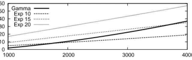
0 10 20 30 40 50 60 1000 2000 3000 4000 Gamma Exp 10 Exp 15 Exp 20

Fig. 2. Simulation time of a chain of exponentially distributed steps vs. the equivalent Erlang step

varying the length of the chain.

The expert reader has already noticed that the distributionTnofθncan be computed

only after computing the distributionTiofθi,0 ≤ i < n. This is essential to correctly

calculate ofPn−1

h=i+1Th. We conclude this section giving a constructive definition of a

stochastic computation.

Definition 5. Given a proved computationξ = B0 θ0

−→ B1 θ1

−→ . . . θn

−→ Bn+1, the

corresponding stochastic computation is

ξn+1= B0 θ0, ˜F0 −→ B1 θ1, ˜F1 −→ . . .θn, ˜Fn −→ Bn+1 defined, fori ≥ 0, as

ξi= if i = 0then ξ else ξi−1{(Bi−1

θi−1 −→ Bi) /(Bi−1 θi−1, ˜Fi−1) −→ Bi} where ˜Fi = P h Ti≤ t +Pi−1h=j+1Th| Tn>Pi−1h=j+1Th i with θj≺Iθi.

3 Experimental Results

We extended theBlenXlanguage and theBetaWBwith a prototypical implementation of the concepts presented in the previous sections. Here we show the effectiveness of the approach by presenting two simple bio-inspired examples that underline the importance of being able to simulate non-Markovian processes.

In the first example we consider the following proved computation:

ξ = B0 θ0

−→ B1 θ1

−→ . . .θ−→ Bn−1 n

whereB0undergoes an n-step transformation becomingBn. Each step is described by

a negative exponential distribution with parameterλ, i.e., $(θi) = 1 − e−λt. A similar

path can be found, for instance, in the lambda phage model described in [17]. If the focus is on simulating the production ofBn , without considering intermediatesBi,

i ∈ [1, n − 1], the system can be approximated as ξA= B0−→ Bθ n

whereθ follows an Erlang distribution with scale λ and shape n, $(θ) = n−1 X j=0 e−λt_(λt)j n!

(11)

Distribution Parameters Mean Variance

Exponential λ = 0.0078 128.2051 16436.554

Erlang k = 2, λ = 0.0156 128.2051 8218.2774

Hyperexponentialp1= 0.3, p2= 0.7 128.2051 79755.80924

λ1= 0.0025, λ2 = 0.085312

Table 3. The three distributions used to model the individual conformational change of proteinA from intermediate to active state.

The abstraction is correct because an Erlang distribution with shapen and scale λ is the

sum ofn exponentially distributed random variables with parameters λ. Fig. 2 shows

the simulation time vs. the number of boxes inB0, whereξ and ξAare simulated with

BetaWB, for different values ofn. Notice that the simulation time of ξAis independent

form the length of the chainn. Moreover, Fig. 2 points out also an argument regarding

the computational efficiency of the simulation, meaning that there are cases in which the use of an Erlang step instead of a chain of exponentially distributed steps is useful not only as a process abstraction, but also for speeding up the simulation time.

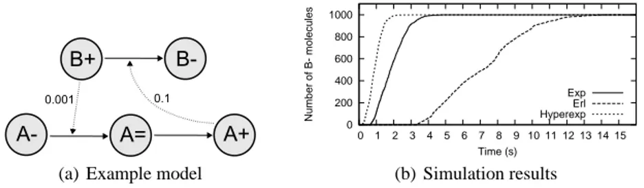
In the second example we consider a simple feedback mechanism (Fig. 3(a)) com-posed of two interacting proteinA and B. Protein B can be in an inactive (B−_{) or}

active (B+_{) form, while protein}_{A can be in an inactive (A}−_{), intermediate (}_A=_{) or}

active (A+_{) form.}_B+_{interact with}_A−_{, transforming it into its intermediate form}_A=_,

which in turn is subject to an individual conformational change that leads to the active formA+_{. Now, consider the individual conformational change. We tried to model this}

reaction in three different ways by using an exponential, an Erlang and a hyperexponen-tial distribution with same means but different variances (see Tab.3). We ran stochastic simulations of the three models with initially a number1000 of B+_and_A−_molecules.

Fig. 3(b) reports simulation results and in particular the number ofB−_{molecules over}

time, showing the speed at which, through the feedback mechanism, the initial amount ofB+ _{is consumed. It is important to note that a different choice in the probability}

distribution that drives the proteinA conformational change has a fundamental impact

on the overall behavior of the system.

(a) Example model

0 200 400 600 800 1000 0 1 2 3 4 5 6 7 8 9 10 11 12 13 14 15 Number of B- molecules Time (s) Exp Erl Hyperexp (b) Simulation results

Fig. 3. Example model and simulation results for the three alternatives using different

(12)

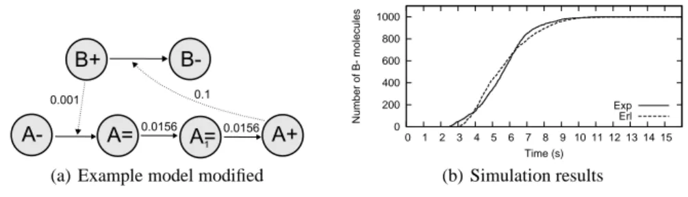
(a) Example model modified 0 200 400 600 800 1000 0 1 2 3 4 5 6 7 8 9 10 11 12 13 14 15 Number of B- molecules Time (s) Exp Erl (b) Simulation results

Fig. 4. Example model with conformational change expressed as a 2-step transformation and

comparison of the simulation results with the one of the model in Fig. 3(a) that uses the Erlang distribution.

Although important itself from a modeling point of view, this fact suggests us that playing with non-Markovian processes is a useful tool to form hypotheses. Consider in-deed a scenario in which the experimental data fits with the simulation results obtained using the Erlang distribution. By the first example we know that our Erlang (Tab.3) can be seen also as a chain of two exponential steps of rateλ = 0.0156, which can lead us to

the hypothesis that maybe our model is incomplete and that the conformational change is a 2-step transformation passing through another intermediate protein formA=

1. This

hypothesis could be used to refine the model in Fig. 3(a) as the one in Fig. 4(a), for which the simulation results in Fig. 4(b) shows the perfect fit with the simulation re-sults for the model in Fig. 3(a) that uses the Erlang distribution, and eventually to drive wet experiments to confirm the hypothesis.

4 Conclusions

We presented the tools to cope with general distributions within theBetaWB frame-work. The proved reduction semantics introduced forBlenXallows us to derive a notion of dependency between transitions without changing theBlenXsyntax. Moreover, we exploit the notion of dependency only for quantitative purposes, but also qualitative as-pects can be retrieved, as, for instance, localities [10]. In the literature there have been many attempts to extend process calculi with general probabilistic distributions (see, e.g., [18–21, 16]), but, to the best of our knowledge, this is the first time an effective simulation tool is available. The examples presented in Sect. 3 outline that reasoning about general distributions could be useful and need further investigations. In particu-lar, the last example proposed non-Markovian processes as a tool to form hypothesis based on experimental observations. Clearly the example is simple and ad-hoc, and a systematic way for constructing hypothesis is needed for validating the approach. Nev-ertheless, the tool presented here is an important step in this direction, because it allows playing with non-Markovian processes at a reasonable computational cost.

(13)

References

1. Milner, R.: Communication and Concurrency. International Series in Computer Science. Prentice hall (1989)

2. Prandi, D., Priami, C., Quaglia, P.: Communicating by compatibility. JLAP 75 (2008) 167 3. Priami, C., Quaglia, P.: Beta binders for biological interactions. In: CMSB 2004. Volume

3082 of LNCS., Springer (2004) 20

4. Meredith, G., Bjorg, S.: Contracts and types. Comm. of the ACM 46(10) (2003) 41–47 5. Tame, J.: Scoring Functions - the First 100 Years. Journal of Computer-Aided Molecular

Design 19 (2005) 445

6. Dematt´e, L., Priami, C., Romanel, A.: The BlenX Language: A Tutorial. In LNCS, ed.: SFM 2008, Springer-Verlag (2008) 313–365

7. Dematt´e, L., Priami, C., Romanel, A.: The Beta Workbench: a computational tool to study the dynamics of biological systems. Briefings in Bioinformatics (2008)

8. Degano, P., Prandi, D., Priami, C., Quaglia, P.: Beta-binders for biological quantitative ex-periments. Electr. Notes Theor. Comput. Sci 164(3) (2006) 101–117

9. Mura, I.: Exactness and Approximation of the Stochastic Simulation Algorithm. Technical Report 12/2008, The Microsoft Research - University of Trento Centre for Computational and Systems Biology (2008)

10. Curti, M., Degano, P., Priami, C., Baldari, C.: Modelling biochemical pathways through enhancedπ-calculus. TCS 325(1) (2004) 111

11. Degano, P., Priami, C.: Enhanced operational semantics: A tool for describing and analysing concurrent systems. ACM Computing Surveys 33(2) (2001) 135–176

12. Guerriero, M.: From Intuitive Descriptions of Biochemical Systems to Their Formal Anal-ysis. PhD in Information and Communication Technologies, International Doctorate School in Information and Communication Technologies – University of Trento (2007)

13. Marsan, M., Balbo, G., Bobbio, A., Chiola, G., Conte, G., Cumani, A.: The Effect of Exe-cution Policies on the Semantics and Analysis of Stochastic Petri Nets. IEEE Transactions on Software Engeneering 15(7) (1989) 832–846

14. Phillips, A., Cardelli, L.: Efficient, Correct Simulation of Biological Processes in the Stochastic Pi-calculus. In: CMSB 2007. Volume 4695 of LNCS., Springer (2007) 184 15. de Bruijn, N.: Lambda calculus notation with nameless dummies. Indagationes

Mathemati-cae 34 (1972) 381–392

16. Priami, C.: Language-based performance prediction for distributed and mobile systems. Information and Computation 175 (2002)

17. Arkin, A., Ross, J., McAdams, H.: Stochastic Kinetic Analysis of Developmental Pathway Bifurcation in Phageλ-Infected Escherichia coli Cells. Genetics 149 (1998) 1633

18. Götz, N., Herzog, U., Rettelbach, M.: TIPP - Introduction and Application to Protocol Per-formance Analysis. In: Formale Methoden für verteilte Systeme, GI/ITG-Fachgespräch, Magdeburg, 10.-11. Juni 1992. (1992) 105–125

19. Marsan, M., Bianco, A., Ciminiera, L., Sisto, R., Valenzano, A.: A LOTOS extension for the performance analysis of distributed systems. IEEE/ACM Transactions Networking 2(2) (1994) 151–165

20. Brinksma, E., Katoen, J., Langerak, R., Latella, D.: A Stochastic Causality-Based Process Algebra. the Computer Journal 38(7) (1995) 552–565

21. Bravetti, M., Bernardo, M., Gorrieri, R.: Towards Performance Evaluation with General Distributions in Process Algebras. In: CONCUR ’98: Concurrency Theory, 9th International Conference, Nice, France, September 8-11, 1998, Proceedings. (1998) 405–422