UNIVERSITY
OF TRENTO
DIPARTIMENTO DI INGEGNERIA E SCIENZA DELL’INFORMAZIONE
38123 Povo – Trento (Italy), Via Sommarive 14
http://www.disi.unitn.it
METAMATERIAL LENSES FOR ANTENNA ARRAYS
LINEAR ARRAY MINIATURIZATION
E. T. Bekele, F. Viani, L. Manica, G. Oliveri and A. Massa
March 2013
Contents
1 Introduction 3
2 Mathematical Formulation 4
2.1 +qTo Library . . . 6
2.2 Grid Orthogonality Assessment . . . 7
3 Numerical Results 8
3.1 Linear Array Scaling . . . 8
1
Introduction
2
Mathematical Formulation
Each one step transformation involves two domains. In this report, the first domain is called “virtual domain” or “virtual space” while the other one is referred to as “physical domain” or “physical space”. In addition, the terms “virtual” and “physical” are used to describe entities in virtual and physical spaces respectively. The rectangular
coordinate system in virtual space is labeled as (x!, y!, z!) whereas in the physical space the labels (x, y, z) are
used.
If the transformation from (x!, y!, z!) to (x, y, z) is defined as:
(x, y, z) = Γ (x!, y!, z!) (1)
x= x (x!, y!, z!) (2)
y= y (x!, y!, z!) (3)
z= z (x!, y!, z!) (4)
the Jacobian matrix of the transformation Λ will be:
Λ = ∂x ∂x! ∂x ∂y! ∂x ∂z! ∂y ∂x! ∂y ∂y! ∂y ∂z! ∂z ∂x! ∂z ∂y! ∂z ∂z! . (5)
For the inverse transformation i.e. (x, y, z) to (x!, y!, z!),
(x!, y!, z!) = Γ!(x, y, z) (6)
x! = x!(x, y, z) (7)
y!= y!(x, y, z) (8)
z!= z!(x, y, z) (9)
the corresponding Jacobian matrix will be
Λ!= ∂x! ∂x ∂x! ∂y ∂x! ∂z ∂y! ∂x ∂y! ∂y ∂y! ∂z ∂z! ∂x ∂z! ∂y ∂z! ∂z . (10)
and the following relations can be established.
det!Λ!" = 1
det(Λ) (12)
If !! and µ! represent permittivity and permeability tensors in virtual medium respectively,
!!= !! xx !!xy !!xz !! yx !!yy !!yz !! zx !!zy !!zz (13) µ!= µ! xx µ!xy µ!xz µ! yx µ!yy µ!yz µ! zx µ!zy µ!zz (14)
corresponding permittivity and permeability tensors in physical space can be computed as follows:
!= Λ ! !ΛT det(Λ) (15) µ= Λ µ !ΛT det(Λ). (16)
If there is a source with current I! and current density J!in virtual space its corresponding image in the physical
space can be computed as [2]
J= Λ J!
det(Λ). (17)
I= I!. (18)
For a cascade of transformations: ˆΓ {(x!!, y!!, z!!) → (x!, y!, z!)} followed by ˜Γ {(x!, y!, z!) → (x, y, z)}, the overall
transformation Γ {(x!!, y!!, z!!) → (x, y, z)} can be formulated as follows. In the following discussion, and in the
remaining of this report, when dealing with cascade of transformations, the space defined by the coordinates
(x!, y!, z!) will be termed as the Intermediate space and objects defined in this space will be called intermediate
objects. Let ˆΛ and ˜Λ represent the Jacobian matrices of the transformations ˆΓ and ˜Γ respectively defined as:
ˆ Λ = ∂x! ∂x!! ∂x! ∂y!! ∂x! ∂z!! ∂y! ∂x!! ∂y! ∂y!! ∂y! ∂z!! ∂z! ∂x!! ∂z! ∂y!! ∂z! ∂z!! (19) ˜ Λ = ∂x ∂x! ∂x ∂y! ∂x ∂z! ∂y ∂x! ∂y ∂y! ∂y ∂z! ∂z ∂x! ∂z ∂y! ∂z ∂z! . (20)
Further more, let )!!!, µ!!*, )!!, µ!*
and {!, µ} represent sets of permittivity and permeability tensors in
J!and J. Considering the transformation: ˜Γ {(x!, y!, z!) → (x, y, z)}, the following relations can be established: != Λ !˜ !Λ˜ T det! ˜Λ" (21) µ= ˜ Λ µ!Λ˜T det! ˜Λ" (22)
and for the other transformation, ˆΓ {(x!!, y!!, z!!) → (x!, y!, z!)},
!!= Λ !ˆ !!Λˆ T det! ˆΛ" (23) µ!= Λ µˆ !!ΛˆT det! ˆΛ" . (24)
Substituting (23) and (24) in (21) and (22) respectively and rearranging terms gives the relationship between material properties for the overall transformation
!= ! ˜ΛˆΛ" !!! ! ˜ΛˆΛ"T det! ˜ΛˆΛ" (25) µ= ! ˜Λ ˆΛ" µ!!! ˜Λ ˆΛ"T det! ˜Λ ˆΛ" . (26)
Following similar analysis, the current sources for the complete transformation can be related as:
J = ! ˜Λ ˆΛ" J!! det! ˜Λ ˆΛ" . (27) I= I! = I!!. (28)
2.1
+qTo Library
The +qTo software library is a numerical implementation of 2D Transformation. It takes boundary contour of virtual space as input and generates grid of transformation to a rectangular region. It first selects points on the input contour in virtual space corresponding to uniformly distributed points on the contour of rectangle in physical space. The internal grid is generated by taking these points as boundary conditions and solving the 2D Laplacian equation. The detail of the solution is presented in [4].
Equations (15) and (16) are used to compute material permittivity and permeability tensors for generic trans-formation. Under the following assumptions, the expression for these quantities can be simplified[5].
• Grid lines are orthogonal.
• Size of mesh elements is equal (square mesh). • Isotropic medium in virtual space.
Under such assumptions, permittivity and permeability in physical space will be simplified as: • For T E mode of propagation:
– Constant permeability: µr(x, y) = µr.
– Isotropic permittivity computed as ratio of the area of the cells of the transformation grid.
• For T M mode of propagation:
– Constant permittivity: !r(x, y) = !r.
– Isotropic permeability computed as ratio of the area of the cells of the transformation grid.
2.2
Grid Orthogonality Assessment
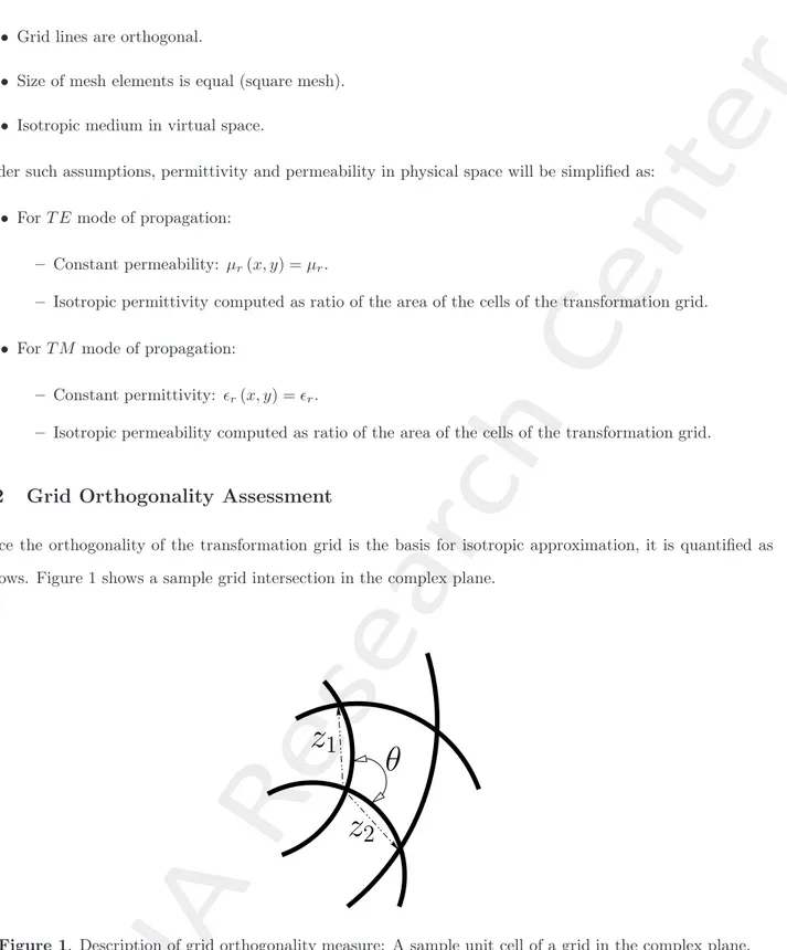
Since the orthogonality of the transformation grid is the basis for isotropic approximation, it is quantified as follows. Figure 1 shows a sample grid intersection in the complex plane.
θ
z
1
z
2
Figure 1. Description of grid orthogonality measure: A sample unit cell of a grid in the complex plane.
Referring to Figure 1, and using Euler’s notation, z1 = |z1| ej[arg(z1)], z2 = |z2| ej[arg(z2)], the internal angle θ
can be computed as
θ= arg (z1) − arg (z2) = arg
! z1
z2
" . The offset from orthogonality χ can then be evaluated as
3
Numerical Results
3.1
Linear Array Scaling
Goal: Reduction of Linear Array aperture size
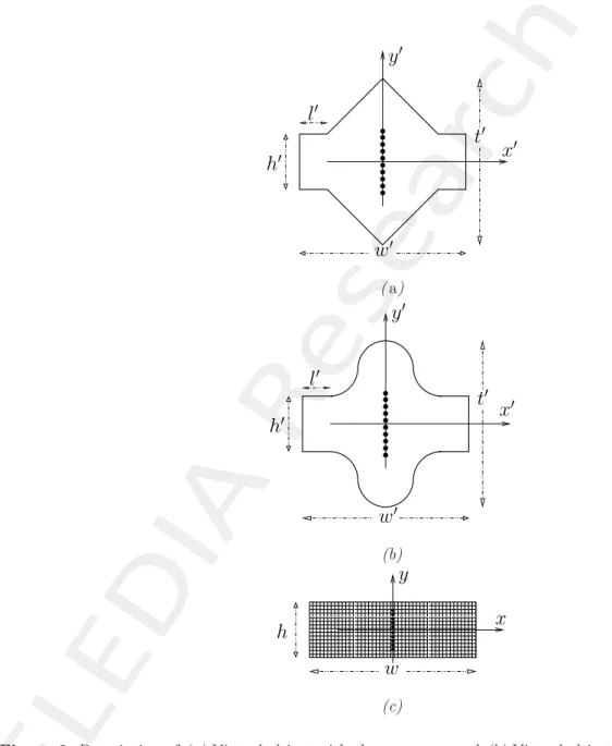
Test Case Description
A 2D problem is considered and the transformation is described pictorially in Figure 2. Figure 2(a) and 2(b) show the setup of the virtual array under investigation. The shape of the smooth transition in Figure 2(b) is defined by one complete period of the cosine function. The region included with the solid curve (Figure 2(a) and 2(b)) is transformed to a rectangular region in the physical space (Figure 2(c)). The shaded region in the physical space (Figure 2(c)) shows the location of metamaterial lens.
y
!x
!l
!t
!w
!h
! ( a)y
!x
!l
!t
!w
!h
! (b)w
x
y
h
(c)Figure 2. Description of (a) Virtual object with sharp corners and (b) Virtual object with smooth transition, and (c) Physical object.
Simulation Parameters
• Array of Isotropic radiators.
• Frequency of operation: ν = 600M Hz • Wavelength in free space: λ = 0.5m Virtual Object Parameters:
• Linear Array of point sources in 2D.
• Width of transformation region: w!= 12λ = 6m.
• Height of transformation region: t! = 16λ = 8m.
• Element Spacing: d! = 0.5λ = 0.25m.
• Uniform Excitation: I!
n= 1, ϕ!n= 0, n = 1, 2, · · · N .
Transformation Parameters:
• Number of grid lines along x!− axis: xgrid = 121.
Full wave simulation Parameters:
• Two dimensional problem. • T E waves.
RESULTS
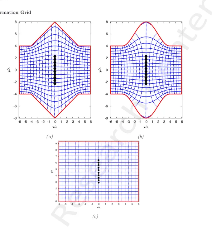
Transformation Grid -8 -6 -4 -2 0 2 4 6 8 -6 -5 -4 -3 -2 -1 0 1 2 3 4 5 6 y/ λ x/λ -8 -6 -4 -2 0 2 4 6 8 -6 -5 -4 -3 -2 -1 0 1 2 3 4 5 6 y/ λ x/λ ( a) (b) 0 1 2 3 4 5 6 7 8 9 -6 -5 -4 -3 -2 -1 0 1 2 3 4 5 6 y/ λ x/λ (c)Figure 3. Transformation Grids: (a) Virtual Space and (b) Physical space.
Observations:
• The medium is discretized into: 92 × 120 cells for sharp corner and 90 × 120 cells for smooth transition. • In physical space each cell has dimensions: 0.1λ × 0.1λ.
• As a result the dimension of the transformation region in physical space is:
– w= 120 × 0.1λ = 12λ, t = 92 × 0.1λ = 9.2λ for transformation with sharp corner and
RESULTS
Grid orthogonality assessment.
(a) (b) 0 1 2 3 4 5 6 7 -16 -14 -12 -10 -8 -6 -4 -2 0 2 4 6 8 10 12 14 16 % of Grid Intersections χ[Degrees] 0 5 10 15 20 25 30 35 40 45 50 55 60 -10 -8 -6 -4 -2 0 2 4 6 8 10 % of Grid Intersections χ[Degrees] (c) (d)
Figure 4. Transformation grid orthogonality test: Transformation with (a),(c) sharp corner, (b),(d) smooth transition.
Observations:
• Large degree of offset from orthogonality is observed.
• The offset is severe around the top and bottom corners. (Figure 4(a)).
RESULTS
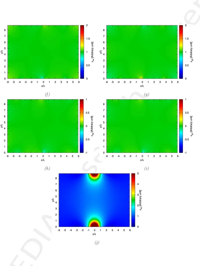
Exact values of permittivity.
Because of the two dimensionality of the problem, some of the parameters related to the z − axis are zero valued (i.e !!
vz= !vz= !!zv = !zv= µ!vz= µvz= µ!zv= µzv= 0 where v ∈ {x, y}). The non-zero valued parameters are
reported next.
(a) (b)
(c) (d)
(f ) (g)
(h) (i)
(j)
Figure 5. Components of the permittivity tensor in the physical medium: Transformation with (a)-(e) sharp
Observations:
• Since the virtual medium is free space (!!
r= µ!r= 1), the permeability tensor in the physical medium, µ
is the same as that of permittivity, i.e µ = !.
• For T E waves, the components of ! and µ that contribute are !zz, µxx, µxy, µyy and µyx.
• The quantities µxy= !xy and µyx= !yx are near zero whereas µxx= !xxand µyy= !yy are near unity.
RESULTS
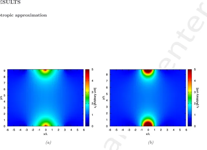
Isotropic approximation
(a) (b)
Figure 6. Isotropic permittivity (!r) of the physical medium computed as ratio of area of transformation
grid: Transformation with (a) sharp corner, (b) smooth transition.
Observations:
• For T E waves, this Isotropic gradient of permittivity (!r) is used.
• This approximation is valid under the assumption that the grids in virtual space are “nearly” orthogonal. Looking at Figure 4, this assumption is better satisfied for the transformation with smooth transition. • Values are bounded:
– 0.0317 ≤ !r≤ 4.936 for transformation with sharp corner (Figure 6(a)).
RESULTS
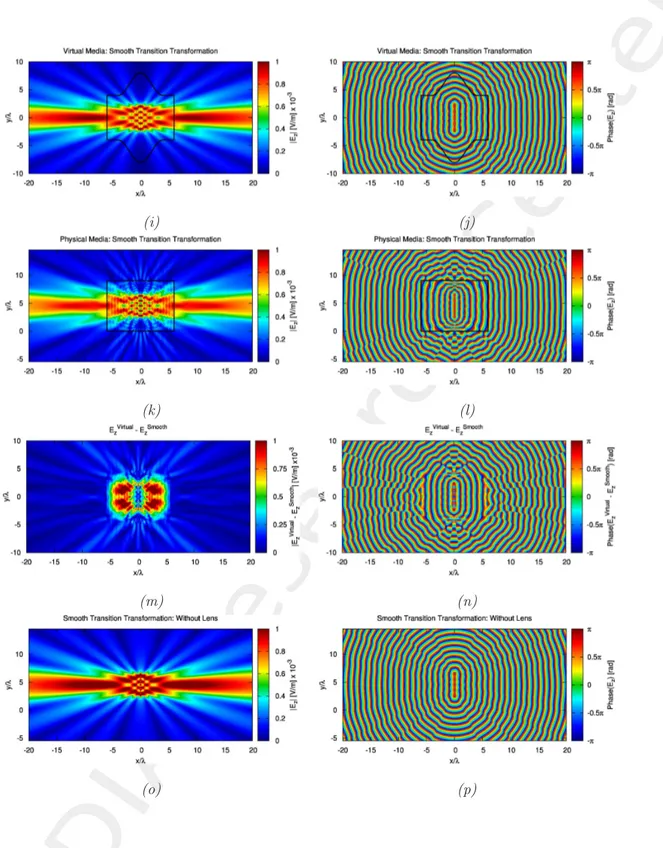
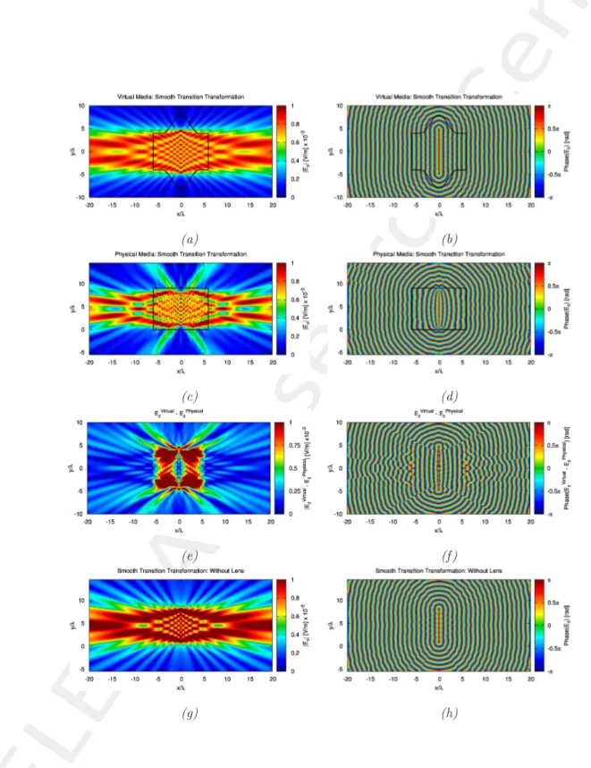
Simulation Results (a) (b) (c) (d) (e) (f ) (g) (h)(i) (j)
(k) (l)
(m) (n)
(o) (p)
Figure 7. Normal component of the electric field: (a), (b) Virtual half wavelength linear array with sharp corners; (c),(d) Transformed linear array with sharp corners; (e),(f) Difference between virtual and transformed array; (g),(h) Transformed linear array in the absence of the metamaterial lens (with sharp corner
transformation); (i), (j) Virtual half wavelength linear array with smooth transition transformation; (k),(l) Transformed linear array with smooth transition transformation; (m),(n) Difference between virtual and transformed array (smooth transition transformation); (o),(p) Transformed linear array in the absence of the
RESULTS
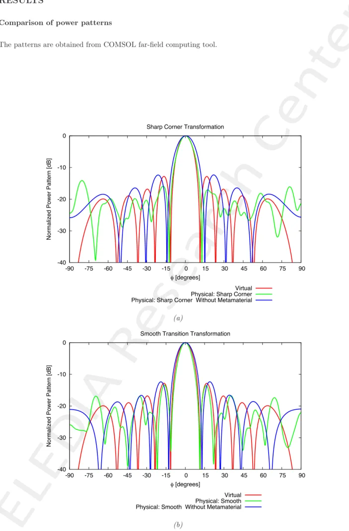
Comparison of power patterns
The patterns are obtained from COMSOL far-field computing tool.
-40 -30 -20 -10 0 -90 -75 -60 -45 -30 -15 0 15 30 45 60 75 90
Normalized Power Pattern [dB]
φ [degrees] Sharp Corner Transformation
Virtual Physical: Sharp Corner Physical: Sharp Corner Without Metamaterial
(a) -40 -30 -20 -10 0 -90 -75 -60 -45 -30 -15 0 15 30 45 60 75 90
Normalized Power Pattern [dB]
φ [degrees]
Smooth Transition Transformation
Virtual Physical: Smooth Physical: Smooth Without Metamaterial
(b)
Observations:
• Comparing Figure 7(e) and Figure 7(m), the transformation with smooth transition gives less error (better match with ideal).
• The patterns of the virtual array and the physical array have good agreement in a limited range ( −15 <
φ <15) Figure 8(a), Figure 8(b). The agreement is much better for the smooth transition transformation.
• The pattern are different outside that limited range. I think this is also because of the mismatch of the transformation region in the upper and lower directions.
RESULTS
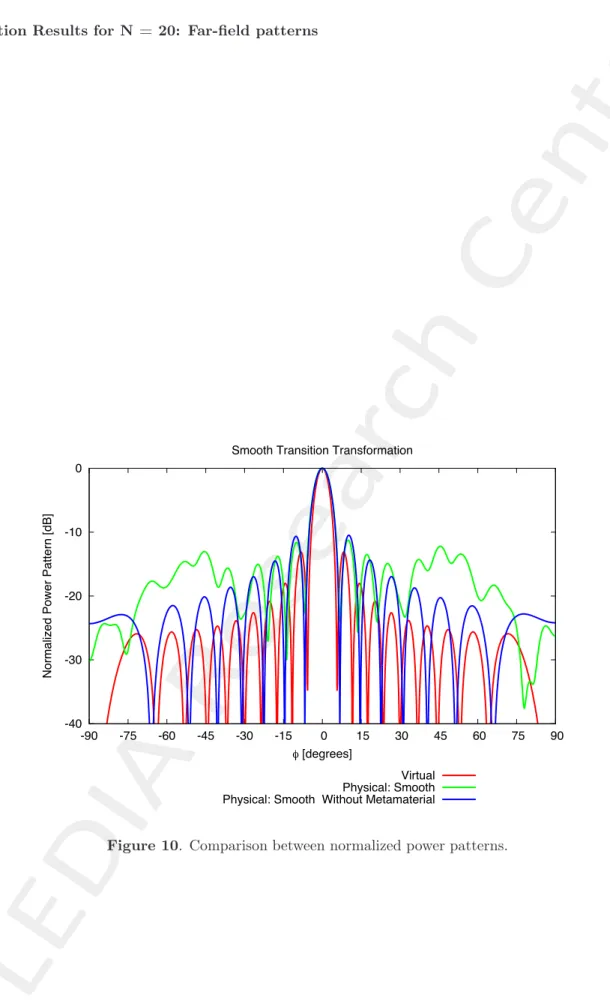
Simulation Results for N = 20
The simulations are repeated using the same transformation setup as in the previous case (transformation with smooth transition), except the number of radiating elements which in this case is N = 20. The simulations are done using smooth transition transformation only.
(a) (b)
(c) (d)
(e) (f )
(g) (h)
Figure 9. Normal component of the electric field: (a), (b) Virtual half wavelength linear array; (c),(d) Transformed linear array; (e),(f) Difference between virtual and transformed array; (g),(h) Transformed linear
RESULTS
Simulation Results for N = 20: Far-field patterns
-40 -30 -20 -10 0 -90 -75 -60 -45 -30 -15 0 15 30 45 60 75 90
Normalized Power Pattern [dB]
φ [degrees]
Smooth Transition Transformation
Virtual Physical: Smooth Physical: Smooth Without Metamaterial
RESULTS
Simulation Results for N = 30
The simulations are repeated using the same transformation setup as in the previous case (transformation with smooth transition), except the number of radiating elements which in this case is N = 30. The simulations are done using smooth transition transformation only.
(a) (b)
(c) (d)
(e) (f )
(g) (h)
Figure 11. Normal component of the electric field: (a), (b) Virtual half wavelength linear array; (c),(d) Transformed linear array; (e),(f) Difference between virtual and transformed array; (g),(h) Transformed linear
RESULTS
Simulation Results for N = 30: Far-field patterns
The patterns are obtained from COMSOL far-field computing tool.
-40 -30 -20 -10 0 -90 -75 -60 -45 -30 -15 0 15 30 45 60 75 90
Normalized Power Pattern [dB]
φ [degrees]
Smooth Transition Transformation
Virtual Physical: Smooth Physical: Smooth Without Metamaterial
Figure 12. Comparison between normalized power patterns.
Observations:
• The error plotted in Figure 11(e) (also in Figure 9(e), Figure 7(m) and Figure 7(e)), is greater in the upper and lower directions (±y direction) from the lens. This could be because the virtual object grid is not matched to the outside space in those directions.
3.2
Resume
N = 10 N = 20 N = 30
Array Type L [λ] BW [degree] L[λ] BW [degree] L[λ] BW [degree]
Virtual Array 4.50 10.27 9.50 5.23 14.50 3.42
Physical Array: Sharp Corner 3.49 9.91 - - -
-Physical Array: Smooth Transition 3.95 8.65 7.38 6.31 8.91 6.85
Without Metamaterial: Sharp Corner 3.49 13.33 -
-Without Metamaterial: Smooth Transition 3.95 11.71 7.38 6.31 8.91 4.86
Tab. I -Parameters of the arrays: Number of Elements (N ), Aperture Length (L), 3dB Beam Width (BW )
Observations:
• As the array size is increased, the matching between virtual and physical array far-field patterns reduces. (Figure 8(b), Figure 10 and Figure 12)
• The error in near-field is also increased when the array size is increased. (Figure 7(m), Figure 9(e) and Figure 11(e))
• The size of the lens has not been scaled in proportion to the array size, and this could be the reason behind the performance degradation.
Acknowledgment
This work has been developed within the EMERALD Project funded by Autonomous Province of Trento - Calls for proposal “Team 2011”.
References
[1] D.-H. Kwon, “Quasi-conformal transformation optics lenses for conformal arrays,” IEEE Antennas Wireless Propag. Lett., vol. 11, pp. 1125-1128, Sept. 2012.
[2] S. A. Cummer, N. Kundtz, and B.-I. Popa, “Electromagnetic surface and line sources under coordinate transformations,” Physical Review Letters A, 80 033820, pp. 033820 1-7, Sept. 2009.
[3] Y. Luo, J. Zhang, L. Ran, H. Chen, and J. A. Kong, “New concept conformal antennas utilizing metama-terial and transformation optics,” IEEE Antennas Wireless Propag. Lett., vol. 7, pp. 509-512, Jul. 2008.
[4] D. C. Ives and R. M. Zacharias, “Conformal mapping and orthogonal grid generation,” In
AIAA/SAE/ASME/ASEE 23rd Joint Propulsion Conference, San Diego, California, Paper number 87-2057, June 1989.
[5] W. Tang, C. Argyropoulos, E. Kallos, W. Song and Y. Hao, “Discrete coordinate transformation for de-signing all-dielectric flat antennas,” IEEE Trans. Antennas Propag., vol. 58, no. 12, pp. 3795-3804, Dec. 2010.
[6] C. A. Balanis, Antenna Theory: Analysis and Design (3rd Ed.). Wiley, 2005.
[7] P. Rocca, M. Benedetti, M. Donelli, D. Franceschini, and A. Massa, "Evolutionary optimization as applied to inverse problems," Inverse Problems - 25th Year Special Issue of Inverse Problems, Invited Topical Review, vol. 25, pp. 1-41, Dec. 2009.
[8] P. Rocca, G. Oliveri, and A. Massa, "Differential Evolution as applied to electromagnetics," IEEE Antennas and Propagation Magazine, vol. 53, no. 1, pp. 38-49, Feb. 2011.
[9] G. Oliveri and A. Massa, "GA-Enhanced ADS-based approach for array thinning," IET Microwaves, An-tennas & Propagation , vol. 5, no. 3, pp. 305-315, 2011.
[10] G. Oliveri, F. Caramanica, and A. Massa, "Hybrid ADS-based techniques for radio astronomy array design," IEEE Transactions on Antennas and Propagation - Special Issue on "Antennas for Next Generation Radio Telescopes," vol. 59, no. 6, pp. 1817-1827, Jun. 2011.
[11] L. Poli, P. Rocca, G. Oliveri, and A. Massa, "Harmonic beamforming in time-modulated linear arrays," IEEE Transactions on Antennas and Propagation, vol. 59, no. 7, pp. 2538-2545, Jul. 2011.
[12] L. Poli, P. Rocca, L. Manica, and A. Massa, "Handling sideband radiations in time-modulated arrays through particle swarm optimization," IEEE Transactions on Antennas and Propagation, vol. 58, no. 4, pp. 1408-1411, Apr. 2010.
[13] L. Poli, P. Rocca, L. Manica, and A. Massa, "Time modulated planar arrays - Analysis and optimization of the sideband radiations," IET Microwaves, Antennas & Propagation, vol. 4, no. 9, pp. 1165-1171, 2010. [14] L. Lizzi, F. Viani, R. Azaro, and A. Massa, "Optimization of a spline-shaped UWB antenna by PSO,"
IEEE Antennas and Wireless Propagation Letters, vol. 6, pp. 182-185, 2007.
[15] L. Lizzi, F. Viani, R. Azaro, and A. Massa, "A PSO-driven spline-based shaping approach for ultra-wideband (UWB) antenna synthesis," IEEE Transactions on Antennas and Propagation, vol. 56, no. 8, pp. 2613-2621, Aug. 2008.
[16] P. Rocca, L. Manica, and A. Massa, "An improved excitation matching method based on an ant colony optimization for suboptimal-free clustering in sum-difference compromise synthesis," IEEE Transactions on Antennas and Propagation, vol. 57, no. 8, pp. 2297-2306, Aug. 2009.
[17] P. Rocca, L. Manica, and A. Massa, "Ant colony based hybrid approach for optimal compromise sum-difference patterns synthesis," Microwave and Optical Technology Letters, vol. 52, no. 1, pp. 128-132, Jan. 2010.
[18] P. Rocca, L. Manica, F. Stringari, and A. Massa, "Ant colony optimization for tree-searching based synthesis of monopulse array antenna," Electronics Letters, vol. 44, no. 13, pp. 783-785, Jun. 19, 2008.
[19] G. Oliveri and L. Poli, "Optimal sub-arraying of compromise planar arrays through an innovative ACO-weighted procedure," Progress in Electromagnetic Research, vol. 109, pp. 27-299, 2010.
[20] G. Oliveri, "Improving the reliability of frequency domain simulators in the presence of homogeneous metamaterials - A preliminary numerical assessment," Progress In Electromagnetics Research, vol. 122, pp. 497-518, 2012.
[21] I. Martinez, A. H. Panaretos, D. Werner, G. Oliveri, and A. Massa "Ultra-thin reconfigurable electro-magnetic metasurface absorbers," 2013 European Conference on Antennas and Propagation (EUCAP), (Gothenburg, Sweden), 8-12 April 2013.
[22] G. Oliveri, P. Rocca, D. H. Werner, E. Bekele, M. Salucci, and A. Massa, "Design and synthesis of innovative metamaterial-enhanced arrays" 2013 IEEE Antennas and Propagation Society International Symposium, (Orlando, USA), July 7-13, 2013.
[23] E. Martini, G. M. Sardi, P. Rocca, G. Oliveri, A. Massa, and S. Maci "Optimization of metamaterial WAIM for planar arrays", 2013 USNC-URSI National Radio Science Meeting, (Orlando, USA), July 7-13, 2013.