A self-organizing map analysis of survey-based agents’
expectations before impending shocks for model selection: The
case of the 2008 financial crisis
Oscar Claveria¹*, Enric Monte², Salvador Torra³
¹ AQR-IREA, University of Barcelona (UB)
² Department of Signal Theory and Communications, Polytechnic University of Catalunya (UPC) ³ Riskcenter-IREA, Department of Econometrics and Statistics, University of Barcelona (UB)
Oscar Claveria
AQR-IREA (Institute of Applied Economics Research) University of Barcelona Diagonal, 690 08034 Barcelona Spain Tel.: +34-934021825 [email protected] Enric Monte
Department of Signal Theory and Communications Polytechnic University of Catalunya
Jordi Girona, 1-3 08034 Barcelona Spain Tel.: +34-934016435 [email protected] Salvador Torra Riskcenter-IREA University of Barcelona Diagonal, 690 08034 Barcelona Spain Tel.: +34-934024318 [email protected]
* Corresponding author. Tel.: +34-934021825; Fax.: +34-934021821. Department of Econometrics,
A self-organizing map analysis of survey-based agents’
expectations before impending shocks for model selection: The
case of the 2008 financial crisis
ABSTRACT
By means of Self-Organizing Maps we cluster fourteen European countries according to the most suitable way to model their agents’ expectations. Using the financial crisis of 2008 as a benchmark, we distinguish between those countries that show a progressive anticipation of the crisis and those where sudden changes in expectations occur. We compare the forecasting performance of Artificial Neural Networks to that of three different time series models and find that neural networks outperform time series models when there are brisk changes in expectations before impending shocks. Conversely, in countries where expectations show a smooth transition towards recession, ARIMA models outperform neural networks. This result demonstrates the usefulness of clustering techniques for selecting the most appropriate method to forecast expectations according to their behaviour.
Keywords: Business surveys; Self-Organizing Maps; Forecasting; Neural networks; Time series
models; Nonlinear models
1. Introduction
Economic expectations play a major role in modern macroeconomics and finance. While economic policy affects expectations (Bernanke et al., 2004), changes in expected future economic activity and their interaction with policy also contribute to fluctuations in macroeconomic aggregates (Leduc and Sill, 2013). Consequently, a large amount of research has been dedicated to investigating the relationship between changes in expectations and economic growth (Zanin, 2010; Claveria et al., 2007; Nolte and Pohlmeier, 2007), obtaining mixed results. Although it remains unclear how economic expectations are formed, anticipating agents’ expectations is of upmost importance in order to assess the current state of the economy, as they are increasingly used as explanatory variables in quantitative forecasting models (Guizzardi and Stacchini, 2015).
Tendency surveys provide detailed information about agents’ expectations. The fact that survey-based expectations are based on the knowledge of the respondents operating in the market and are rapidly available, makes them very valuable for forecasting purposes and decision-making. Survey results are presented as weighted percentages of respondents expecting a variable to go up, to go down or to remain unchanged. The qualitative nature of survey results has often lead to quantify agents’ responses making use of survey indicators, such as the balance statistic. See Lahiri and Zhao (2015) for an appraisal of alternative measures of economic expectations.
The aim of this study is to analyse the role of clustering techniques in order to select the most indicated method to model agents’ expectations according to their perceptions on the state of the economy before imminent shocks. By means of Self-Organizing Maps (SOMs) we map the evolution of economic experts’ expectations during the transition to the 2008 recession. This technique allows us to classify the fourteen European countries into two groups according to the changing perceptions of their economic experts during the pre and post-crisis quarters: those in which the shock is gradually anticipated, vis-à-vis those where a brisk change in expectations occurs.
With focus on the financial crisis of 2008, we then generate predictions of experts’ expectations for fourteen European countries during this transition period and compare the forecasting performance of Artificial Neural Networks (ANNs) to that of three different time series models: autoregressions (AR), autoregressive integrated moving average (ARIMA) and self-exciting threshold autoregressions (SETAR).
Finally, by overlapping the forecasting results with the two clusters obtained in the SOM analysis, we find that the most suitable way to model expectations in each country is connected to the behaviour of experts’ perceptions before the impending crisis.
SOMs use unsupervised training algorithms and belong to a general class of ANNs based on nonlinear regression techniques that can be trained to organize data so as to disclose unknown patterns or structures (Deboeck and Kohonen, 1988). SOMs have been used in order to make visual predictions of different phenomena, but only recently in economic studies (Sarlin and Peltonen, 2013; Resta, 2012; Lu and Wang, 2010; Marghescu et al., 2010; Arciniegas-Rueda and Arciniegas, 2009; Eklund et al., 2008). In this study we make use of SOMs to analyse experts’ expectations about the state of the economy in fourteen European countries before and after the financial crisis of 2008. SOMs allow us to cluster all countries according to the degree to which their experts’ anticipated the crisis and to analyse whether there are significant differences across countries regarding the behaviour of agents’ expectations.
To our knowledge, this is the first study to conduct a SOM analysis to expectations measured by survey indicators. We use the raw data from all the indicators of the three main variables of the World Economic Survey (WES) carried out quarterly by the Ifo Institute for Economic Research: the country’s general situation regarding overall economy, capital expenditures and private consumption. We focus on the question regarding the expected situation by the end of the next six months. The data set includes 18 quarterly indicators and 18 quarterly composite indicators (balance and weighted balance statistics) of each country for the period ranging from 1989 to 2008.
ANNs have powerful pattern classification capabilities (Sarlin and Marghescu, 2011), but are increasingly used with forecasting purposes (Claveria et al., 2014). ANNs have been applied in many fields (Bahmanyar and Karami, 2014; Kang and Cho, 2014; Kaushika et al., 2014), but never before for the short-run forecasting of Business Survey Indicators. As far as we know, only two previous studies have conducted forecast competitions for business survey indicators (Clar et al., 2007; Ghonghadze and Lux, 2009). Such an exercise allows to select the forecasting technique that shows the best forecasting performance (Hendry and Clements, 2003; Stock and Watson, 2003).
Expectations forecasts can then be used to predict business cycle turning points (Qi, 2001; Diebold and Rudebusch, 1989), to quantify business survey data (Lahiri and Zhao, 2015; Breitung, and Schmeling, 2013; Claveria et al., 2006; Mitchell, 2002; Mitchell et
Graff, 2010; Mitchell et al., 2005; Claveria et al., 2007, 2010; Parigi and Schlitzer, 1995; Biart and Praet, 1987). Recently, Dees et al. (2013) empirically assesses the link between the consumer sentiment indicator and consumer expenditures in the United States and the Euro Area.
Many authors have acknowledged the importance of applying new approaches to forecasting in order to improve the accuracy of the methods of analysis (Buchen and Wohlrabe, 2013; Robinzonov et al., 2012; Song and Li, 2008). Silva and Hassani (2015) evaluate the impact of the 2008 recession on US trade by means of Singular Spectrum Analysis (SSA). The availability of more advanced forecasting techniques has led to a growing interest Artificial Intelligence (AI) methods (Gharleghi et al., 2014; Cang, 2014; Pai et al., 2014; Celotto et al., 2012; Chen, 2011; Lin et al., 2011; Goh et al., 2008; Yu and Schwartz, 2006) to the detriment of time series models (Chu, 2008, 2011) and causal econometric models (Franses et al., 2011). Some of the most commonly used AI-based techniques in economics and finance are fuzzy time series models (Tsaur and Kuo, 2011), Support Vector Machines (SVMs) (Kao et al., 2013) and ANNs. Recent research has shown the suitability of ANNs for dealing with time series forecasting (Fioramanti, 2008; Sermpinis et al., 2012; Claveria and Torra, 2014).
ANNs can be classified into feed-forward networks and recurrent networks depending on the connecting patterns of the different layers of neurons. In feed-forward networks the information runs only in one direction, whilst in recurrent networks there are feedback connections from outer layers of neurons to lower layers of neurons. Feed-forward networks were the first ANNs devised. The Multi-layer perceptron (MLP) network is the most widely used feed-forward topology in time series forecasting (Lin et al., 2011, Palmer et al., 2006; Kon and Turner, 2005; Zhang and Qi, 2005; Tsaur et al., 2002). In this paper we use a MLP architecture to forecast the expectations of the WES. SOMs are feed-forward ANNs that use unsupervised training algorithms and belong to a general class of ANNs based on nonlinear regression techniques that allow to generate topological representations of the original data.
The structure of the paper is as follows. Section 2 presents our methodological approach and describes the forecasting models. The results of the forecasting competition are described in Section 3. In Section 4 we combine a SOM analysis of all the information and the forecasting results. Conclusions are given in Section 5.
2. Methodology
In this section we present the different AI-based techniques and the time series models used in the study. We use two types of ANNs in the analysis: MLP networks are used to generate forecasts of survey indicators, while SOMs allow us clustering
European countries according to the forecasting results and to their agents’ perceptions in order to find behavioural patterns of expectations.
2.1. Artificial Neural Networks
ANNs are an AI-based technique that consist of interconnected processing units called neurons. They have a parallel distribution information processing device that allows them to approximate the mapping between input and output by nonlinear functions. ANNs learn from experience and they are able to capture functional relationships when the underlying process is unknown, as it happens with the data generating process of economic expectations. These features have brought us to use SOMs in order to cluster European countries according to their experts’ expectations regarding the state of the economy during the crisis of 2008, which in turn allows us to test whether differences in expectations’ behavior have an effect on the modeling procedure used to generate forecasts from tendency survey indicators.
The fact that ANNs are able to identify related temporal patterns by learning from historical data explains the great interest that ANNs have aroused for economic forecasting (Feng and Zhang, 2014; Kock and Teräsvirta, 2011, 2014; Pérez-Rodríguez et al., 2005, 2009; Nakamura, 2005; Qi, 2001; Cybenko, 1989; Funahashi, 1989; Hornik, Stinchcombe and White 1989; Wasserman, 1989, Adya and Collopy, 1998; Swanson and White, 1997; Kaastra and Boyd, 1996; Hill, Marquez, O’Connor and Remus, 1994). In the present study we compare the forecasting performance of a MLP ANN to that of different time series models, and we select the most suitable methodology to model and forecasts expectations based on the behavior recorded.
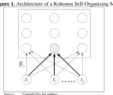
A SOM is a special type of feed-forward ANN model that uses an unsupervised learning algorithms based on the idea of the similarity between inputs and weights (Kohonen, 1982, 2001). SOMs may be considered a nonlinear generalization of Principal Components Analysis (PCA) that have many advantages over the conventional feature extraction methods (Liu and Weisberg, 2005). SOM models consist of a two-layer architecture: in the first layer (input layer) information is distributed, while in the second layer (output layer) the representation is made. The final output is usually represented in a two-dimensional map of neurons (see Figure 1). Therefore, SOMs can be regarded as representations of similitude relations in data.
Figure 1. Architecture of a Kohonen Self-Organizing Map
Source: Compiled by the authors.
Figure 1 represents the architecture of a Kohonen network, in which each column in the grid represents a neuron. Each neuron has as many weights as the input descriptors for the objects to be mapped into the network. The training phase in a SOM consists of adjusting the weights in a competitive iterative process. The winning neuron is that with the most similar weights to the input descriptors. The weights are then corrected so that they become more similar to the input descriptors (measured by the smallest distance metric). Then neurons are classified during the mapping phase according to the type of the objects that are mapped. This process allow SOMs for a nonlinear projection of a high-dimensional space (inputs) onto a discrete space (output) represented by the wining neurons. Therefore, SOM analysis can be regarded as method for exploratory data analysis that illustrates data structures in easily understandable forms.
The most widely used ANN in time series forecasting is the MLP, which is a supervised network. The MLP architecture is based on the original simple perceptron model, but with additional hidden layers of neurons between the input and output layers that increases the learning power of the network. The number of hidden neurons determines the network’s capacity to learn. Selecting the network which performs best with the least possible number of hidden neurons is most recommended (Bishop, 1995). In this work we used the MLP specification suggested by Kuan and White (1994):
β j q
q j p i φ φ φ x g β β f x j ij j ij t j q j t , , 1 , , , 1 , , , 1 , 0 1 1 0 (1)where f is the output function; g is the activation function; p is the number of inputs;
q is the number of neurons in the hidden layer;
x
t is the output;x
t1 is the input;β
j arethe weights connecting the output with the hidden layer and
φ
ij are the weights connectingthe input with the hidden layer.
Kock and Teräsvirta (2011) and Zhang et al. (1998) review the main ANN modelling issues. We use a MLP
1;3 architecture that allows us to represent the possible nonlinearrelationship between
x
t andx
t1. Once the topology of the neural network is decided, the parameters of the network are estimated by means of different algorithms based on gradient search. Following Ripley (1996), we divide the data into three sets: training, validation and test sets. This division seeks to improve the performance of the network with new cases. Based on these considerations, the period from 1989.I to 2001.IV is selected as the training set (66%), 2002.I to 2006.IV as the validation set (25%) and 2007.I to 2008.IV as the testing set (10%). We use Levenberg-Marquardt algorithm in order to calculate the weights in each of the iterations.2.2. Time series models
We use three different time series models to obtain forecasts for Business Surveys Indicators: autoregressions (AR), integrated moving-average models (ARIMA) and
self-exciting threshold autoregressions models (SETAR). In order to determine the number of lags that should be included in the model, we have selected the model with the lowest value of the Akaike Information Criteria (AIC) considering models with a minimum number of 1 lag up to a maximum of 8 quarters (including all the intermediate lags).
We first considered autoregressions. AR models explain the behaviour of the endogenous variable as a linear combination of its own past values:
t p t p t t t
x
x
x
x
1 1
2 2
...
(2) ARIMA models were first proposed by Box and Jenkins (1970). The general expression of an ARIMA model is the following:
D d t s s s s s t L L L L x (3)where s
Ls 1sLs 2sL2s ...QsLQs
is a seasonal moving averagepolynomial,
s
L
s
1
sL
s
2sL
2s
...
PsL
Ps
is a seasonal autoregressive polynomial,
L
L 2L2...qLq
1 1
1 is a regular moving average polynomial,
and
L
11L12L2...pLp
is a regular autoregressive polynomial, is thevalue of the Box-Cox (1964) transformation,
Ds is the seasonal difference operator, dis the regular difference operator, s is the periodicity of the considered time series (s = 4 for quarterly data), and
t is the innovation which is assumed to behave as a white noise.As Clements and Smith (1999) and Hansen (1997) stated, there seems to be a cyclical asymmetry in the behaviour of most economic variables. A Self-Excited Threshold Autoregressive model (SETAR) for the time series
x
t can be summarised as follows:t t
u
x
L
B
(
)·
ifx
tk
x
(4) t tv
s
L
)·
(
ifx
tk
x
(5)where
u
t andv
t are white noises, B( L) and ( L) are autoregressive polynomials, the value k is known as delay and the valuex
is known as threshold. This two-regime self-exciting threshold autoregressive process is estimated for each indicator and the Monte Carlo procedure is used to generate multi-step forecasts. The values of the threshold are given by the variation of the analysed variable.3. Self-Organizing Map Analysis of agents’ expectations
In the present study we use agent’s expectations from the World Economic Survey (WES) carried out quarterly by the Ifo Institute for Economic Research. The survey questionnaire focuses on qualitative information: assessments of a country’s general situation and expectations regarding important economic indicators. The survey results are published as aggregated data. The aggregation procedure is based on country classifications. Within each country group or region, the country results are weighted according to the share of the specific country’s exports and imports in total world trade (CESifo World Economic Survey, 2011). For a detailed analysis of WES data see Stangl (2008).
Survey results are presented as weighted percentages of respondents expecting a variable to go up, to go down or to remain unchanged. As a result, tendency surveys contain two pieces of independent information at time t, Rt and Ft, denoting the percentage of respondents at time t1 expecting an economic variable to rise or fall at time t. The information therefore refers to the direction of change but not to its magnitude. The qualitative nature of survey results has often lead to quantify them making use of business survey indicators. The most commonly used indicator to present survey results is the balance statistic:
F R
Bt t (6)
Assuming that the expected percentage change in a variable remains constant over time for agents reporting an increase and for those reporting a decrease, Anderson (1951) defined the balance statistic as a measure of the average changes expected in the variable. As the balance statistic (Bt) does not take into account the percentage of respondents expecting a variable to remain constant (Ct), Claveria (2010) proposed a nonlinear variation of the balance statistic (WBt, weighted balance) that accounts for this percentage of respondents: t t t t t t t C B F R F R WB 1 (7)
Weighting the balance statistic by the proportion of respondents expecting a variable to rise or fall allows discriminating between two equal values of the balance statistic depending on the percentage of respondents expecting a variable to remain constant.
A SOM network has the ability to learn and detect regularities and correlations in the inputs. SOMs learn to recognize groups of similar input vectors in such a way that neurons physically near each other in the neuron layer respond to similar input vectors. Their representations are based on the underlying distribution and topology of the input vectors they are trained on. Therefore a SOM can be regarded as method for exploratory data analysis that illustrates data structures in easily understandable forms.
In this study we make use of these features of SOMs to characterize the temporal evolution of the expectations before and during the beginning of the financial crisis of 2008. Our data set encompasses answers from year 1989 to year 2008. In order to assess the capacity of the network to model the behaviour of the expectations, we divide the database into a training database, which consists of the first 73 samples per country (from the first quarter of year 1989 to the fourth quarter of the year 2006), and 8 samples per country for testing (from the first quarter of 2007 to the fourth quarter of 2008). Therefore, the SOM is trained with data from all 14 countries in the aforementioned period.
SOMs cluster data, but also have the property of arranging the clusters by similarity on a plane. Therefore there is an interpolation aspect in the estimation of the centroids. In order to make use of this property, and to have enough granularity on the map, we take a 1010 topology, which yielded 100 centroids and approximately 10 samples per centroid. In order to capture well the topological property of neighbourhood of the centroids, we use an alpha that ranges from 0.05 to 0.0001 along 15000 iterations of the algorithm. The neighbourhood function is taken to be rectangular. We use Python and the 'Kohonen' package implemented in R (Wehrens and Buydens, 2007).
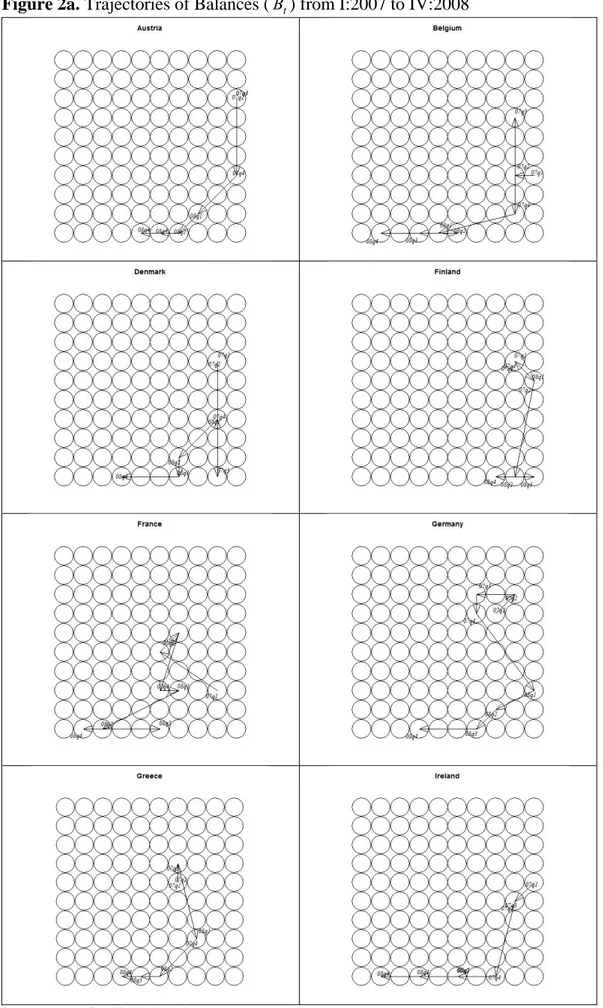
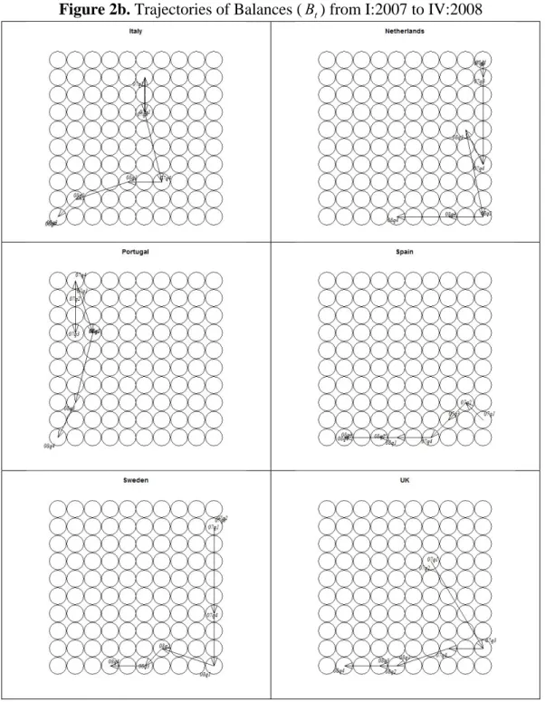
For the test database, we present the trajectories of each country along the nearest centroids for each sample (Figure 2a and 2b). This analysis is based on overlapping the temporal evolution of the agents' expectations on a map. Figures 2a and 2b show the evolution of expectations represented by the balance statistic at the beginning of the 2008 financial crisis in fourteen countries of the European Union (Austria, Belgium, Denmark, Finland, France, Germany, Greece, Ireland, Italy, the Netherlands, Portugal, Sweden and the United Kingdom). These maps allow us to determine different trajectories in order to discriminate between countries with respect of their agents’ perception of the imminent crisis. In most countries we find a tendency that gravitates towards the low right side of the map.
Figure 2a. Trajectories of Balances (Bt) from I:2007 to IV:2008
Figure 2b. Trajectories of Balances (Bt) from I:2007 to IV:2008
Source: Compiled by the authors.
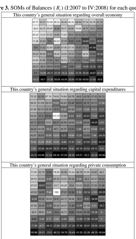
The SOMs in Figure 3 simultaneously map the information regarding the balances for each of the three questions and experts’ expectation. Each grid consists of 100 neurons of different sign. The positive signs indicate the prevalence of positive expectations with regard of negative expectations. The negative signs represent the reverse situation: there are more respondents expecting a decrease in the variable than respondents expecting an increase. The darker the cell, the higher the negative value of the neuron.
The maps in Figure 3 allow us to distinguish between zones of maximum consensus (balances are similar) and zones where expectations present a wider range of discrepancy. The black and white neurons, unlike the grey ones, indicate maximum consensus, regardless of the sign. Therefore, the darker areas represent the predominance of negative expectations. When analysing the distribution for each type of expectation, we find a similar pattern for each question regarding the location of the blackest zones, as most black cells are located on the low side of the map, and gravitate towards the right side.
Figure 3. SOMs of Balances (Bt) (I:2007 to IV:2008) for each question
This country’s general situation regarding overall economy
This country’s general situation regarding capital expenditures
This country’s general situation regarding private consumption
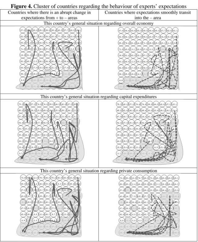
Finally, in Figure 4 we cross temporal information with the SOM analysis displayed in Figures 2 and 3. More specifically, we overlap the trajectories of the expectations for the next six months from the first quarter of 2007 to the last quarter of 2008 on a different map for each of the three questions. The grey zones capture the areas in which there is a predominance of negative expectations. The arrowheads coincide with the last period of analysis (IV:2008), once the perception of the crisis had definitely settled in all countries.
Figure 4. Cluster of countries regarding the behaviour of experts’ expectations
Countries where there is an abrupt change in expectations from + to – areas
Countries where expectations smoothly transit into the – area
This country’s general situation regarding overall economy
This country’s general situation regarding capital expenditures
This country’s general situation regarding private consumption
Using the financial crisis of 2008 as a benchmark, Figure 4 allows us to classify countries into two clusters: those that show a progressive anticipation of the imminent crisis, and those where expectations show a more erratic path prior to reaching a consensus on the entry into recession. The trajectories on the maps of the left side of Figure 4 show abrupt oscillations between the white area and the grey area, while the opposite is true for the trajectories on the three maps of the right side. On the one hand, we find that Italy, the Netherlands and Portugal systematically fall within the second category for all three questions (the country’s general situation regarding overall economy, capital expenditures and private consumption). This result may be indicating a bias toward optimism on the part of agents in some countries. On the other hand, Belgium, Denmark, France, Greece, Ireland, Spain and the United Kingdom present more stable expectations, showing a smooth transition from the period previous to the recession to the post-crisis quarters.
4. Survey Indicators Forecasts
The experiment is based on all the information available for the first three questions of the WES: the country’s general situation regarding overall economy, capital expenditures and private consumption. We use information from fourteen countries of the EU. In order to evaluate the relative forecasting accuracy of the different techniques, each model is estimated for all the indicators included up to 2007.IV and one quarter ahead forecasts are computed in a recursive way. To evaluate the forecasting performance of the different models we compute the Root Mean Square Error (RMSE).
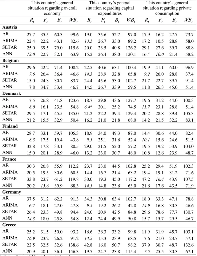
In Tables 1a and 1b we present the main results of the time series prediction experiment, using the last eight quarters for comparing the forecasting accuracy of the different techniques (AR, ARIMA, SETAR and ANN models). We find that ARIMA and ANN models clearly outperform SETAR and AR models. These results differ from those obtained by Clar et al. (2007), who find that the univariate autoregressions were not outperformed by other time series models for the Euro Area. The lowest RMSE values for the expectations regarding the overall economy and private consumption are obtained with ARIMA models in Spain. For the the expectations regarding capital expenditures, the lowest RMSE value is obtained with an ARIMA model for Denmark.
Table 1a. RMSE – Recursive forecasts from I:2007 to IV:2008
Expected situation by the end of the next 6 months This country’s general
situation regarding overall economy
This country’s general situation regarding capital
expenditures
This country’s general situation regarding private
consumption t R Ft Bt WBt Rt Ft Bt WBt Rt Ft Bt WBt Austria AR 27.7 35.5 60.3 99.6 19.0 35.6 52.7 97.0 17.9 16.2 27.7 73.7 ARIMA 22.4 22.2 43.1 82.6 13.5 26.7 33.0 89.2 17.2 10.5 28.8 58.0 SETAR 25.0 39.5 79.0 115.6 20.0 23.5 40.8 126.2 29.1 27.6 39.7 88.8 ANN 12.0 22.7 32.1 63.9 15.2 26.4 38.0 120.1 16.4 10.0 21.4 58.2 Belgium AR 29.6 42.2 71.4 108.2 22.5 40.6 63.1 100.4 19.9 41.1 60.0 96.9 ARIMA 7.6 26.4 36.4 46.6 14.3 28.9 32.8 65.8 9.2 26.0 28.8 37.4 SETAR 15.0 24.3 30.7 83.7 24.4 45.6 53.0 102.7 21.7 22.7 39.7 91.4 ANN 7.8 34.7 33.4 46.7 14.5 26.7 33.9 59.5 11.8 26.3 45.0 51.4 Denmark AR 17.5 26.8 41.8 123.6 18.7 29.8 43.6 127.7 19.6 31.2 44.0 100.3 ARIMA 8.0 16.1 23.5 54.8 6.4* 20.1 25.2 74.5 11.7 23.1 28.8 51.4 SETAR 29.5 17.1 45.5 135.0 21.2 22.2 39.4 129.4 20.2 28.8 39.4 105.3 ANN 21.2 15.5 32.9 50.4 16.2 21.0 21.8 68.0 14.2 21.5 32.2 83.1 Finland AR 28.7 33.1 59.7 105.3 18.9 34.0 49.3 87.0 14.4 30.6 44.0 82.4 ARIMA 8.3 17.5 19.4 43.8 9.3 25.1 31.6 52.4 10.1 15.6 24.6 51.5 SETAR 32.8 17.8 33.1 80.5 29.0 21.5 52.0 57.2 19.5 19.2 53.9 104.0 ANN 15.0 20.1 28.9 46.0 13.2 23.0 30.7 48.0 10.8 12.6 23.9 48.7 France AR 30.3 26.8 55.9 112.2 23.7 23.0 44.5 102.8 25.2 29.4 51.9 102.3 ARIMA 20.5 19.5 30.6 60.5 14.4 16.7 21.4 63.2 19.4 19.1 31.2 71.6 SETAR 33.8 23.7 61.2 119.8 30.0 19.3 45.0 117.2 47.2 16.4 43.9 107.5 ANN 20.2 15.6 39.9 68.3 14.3 14.8 23.6 63.0 21.6 17.6 43.5 71.9 Germany AR 37.5 31.2 62.2 91.3 34.3 30.8 63.4 102.7 18.0 33.3 47.1 78.8 ARIMA 16.7 18.1 27.0 47.8 9.5 19.2 26.2 42.8 14.9 16.8 30.3 46.6 SETAR 26.4 23.3 49.8 94.4 24.0 20.9 42.5 84.8 29.6 78.6 77.7 130.7 ANN 14.3 18.0 25.8 54.8 12.4 24.4 49.9 50.8 15.7 15.7 29.5 46.7 Greece AR 25.2 31.5 50.0 93.2 16.6 36.3 33.2 99.8 11.9 31.9 45.7 103.1 ARIMA 16.9 23.2 26.2 91.2 13.2 15.3 23.9 68.5 7.6 21.0 23.7 57.1 SETAR 22.5 32.5 32.6 138.6 42.8 16.0 50.7 98.2 37.9 30.7 48.7 132.6 ANN 20.9 40.1 36.1 156.3 19.7 24.7 23.8 115.4 7.5 25.5 30.3 67.1 Italics: Best model for each question in each country.
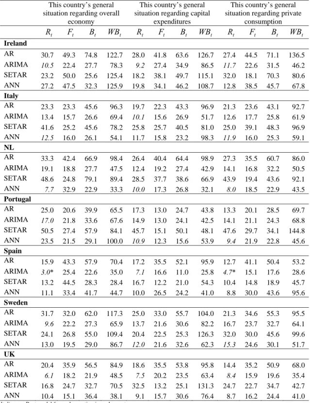
Table 1b. RMSE – Recursive forecasts from I:2007 to IV:2008
Expected situation by the end of the next 6 months This country’s general
situation regarding overall economy
This country’s general situation regarding capital
expenditures
This country’s general situation regarding private
consumption t R Ft Bt WBt Rt Ft Bt WBt Rt Ft Bt WBt Ireland AR 30.7 49.3 74.8 122.7 28.0 41.8 63.6 126.7 27.4 44.5 71.1 136.5 ARIMA 10.5 22.4 27.7 78.3 9.2 27.4 34.9 86.5 11.7 22.6 31.5 46.2 SETAR 23.2 50.0 25.6 125.4 18.2 38.1 49.7 115.1 32.0 18.1 70.3 80.6 ANN 27.2 47.5 32.3 125.9 19.8 34.1 46.2 108.7 12.8 38.5 45.7 67.8 Italy AR 23.3 23.3 45.6 96.3 19.7 22.3 43.3 96.9 21.3 23.6 43.1 92.7 ARIMA 13.4 15.7 26.6 69.4 10.1 15.6 26.9 51.7 12.6 17.7 25.8 61.9 SETAR 41.6 25.2 45.6 78.2 25.8 25.7 40.5 81.0 25.0 39.1 48.3 96.9 ANN 12.5 16.0 26.1 54.1 11.7 15.8 23.2 98.3 11.9 16.0 25.3 59.1 NL AR 33.3 42.4 66.9 98.4 26.4 40.4 64.4 98.9 27.3 35.5 60.7 86.0 ARIMA 19.1 18.8 27.7 47.5 12.4 19.2 27.4 42.9 14.1 16.8 32.2 50.5 SETAR 48.6 24.8 79.1 89.4 28.5 37.7 38.6 66.9 43.9 19.4 43.6 92.1 ANN 7.7 32.9 22.9 33.3 10.0 17.3 26.8 32.1 8.0 18.5 22.9 43.5 Portugal AR 25.0 20.6 39.9 65.5 17.3 13.0 24.7 43.8 13.3 20.1 28.5 69.7 ARIMA 17.0 21.8 33.6 67.6 14.9 13.0 24.1 42.5 14.1 21.1 24.3 68.8 SETAR 50.5 27.4 57.9 84.1 45.7 15.1 50.1 48.1 47.6 29.7 34.1 144.8 ANN 23.5 21.5 29.1 100.0 10.9 12.3 15.6 53.9 9.4 21.9 22.8 45.6 Spain AR 15.9 43.3 57.9 70.4 17.2 35.5 52.1 95.9 12.7 41.1 50.4 53.2 ARIMA 3.0* 25.4 22.6 35.0 7.1 16.6 11.0 25.8 4.7* 15.1 17.6 28.6 SETAR 13.2 44.5 28.3 28.4 16.7 12.2 21.0 54.3 10.4 14.8 18.9 45.7 ANN 11.1 33.4 41.7 44.7 10.0 26.5 24.2 41.0 8.8 30.0 43.6 95.6 Sweden AR 31.7 32.0 62.0 117.3 25.0 33.0 55.7 104.0 21.3 34.6 55.3 95.5 ARIMA 9.6 22.2 27.3 65.9 13.7 21.6 30.6 82.2 16.7 23.7 32.7 64.1 SETAR 24.1 26.8 55.0 109.4 20.4 22.5 25.3 126.3 32.0 30.0 45.6 99.6 ANN 13.0 19.5 29.0 86.7 12.0 21.6 32.6 62.3 15.3 24.6 30.1 51.7 UK AR 20.4 35.9 56.5 84.9 18.6 35.5 53.8 95.8 14.4 35.2 50.9 68.0 ARIMA 6.1 18.2 21.9 48.5 7.5 20.2 23.5 63.4 8.4 15.9 19.6 35.4 SETAR 16.8 24.7 32.7 70.5 32.5 13.2 25.1 131.3 24.7 22.7 34.7 42.7 ANN 10.4 15.1 36.4 38.1 9.1 15.7 30.6 76.4 8.7 16.2 24.4 41.0 Italics: Best model for each question in each country.
We also find that Tendency Survey Indicators (Rt, and Ft) display better forecasts than the aggregates (Bt and WBt). Clar et al. (2007) also find that indirect measures show the best forecasting performance. Specifically, the indicator with the percentage of respondents expecting the variable to rise (Rt) shows the best forecasting performance, for all questions and countries. Taking into account that Rt and Bt are usually highly correlated (Claveria et al., 2003), it might be appropriate to use this indicator as a proxy for agents’ expectations when used as explanatory variables in quantitative forecasts models.
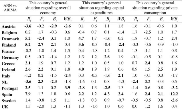
Finally, we apply the Diebold-Mariano test (Table 2) for significant differences between the two best forecasting models for each indicator and variable. When testing for significant differences between ANN and ARIMA models for each two competing series, we find that the differences between both models are more pronounced for the question regarding the overall economy.
Table 2. RMSE – Diebold-Mariano loss-differential test statistic for predictive accuracy ANN vs.
ARIMA
This country’s general situation regarding overall
economy
This country’s general situation regarding capital
expenditures
This country’s general situation regarding private
consumption t R Ft Bt WBt Rt Ft Bt WBt Rt Ft Bt WBt Austria -3.6 -0.2 -2.9 -2.6 0.1 0.6 1.1 1.8 1.6 -0.1 -0.6 1.0 Belgium 0.2 1.7 -0.3 0.6 -0.4 0.7 0.1 -1.4 1.7 -2.5 1.0 1.7 Denmark 5.2 -2.4 3.1 1.0 4.7 1.7 -1.6 0.2 1.8 -0.7 1.2 2.4 Finland 5.2 2.7 2.1 0.4 3.6 -0.3 -0.4 -2.4 -0.3 -0.6 -0.9 -1.0 France -0.2 -1.0 1.4 1.5 0.4 -1.8 1.2 0.4 1.3 -1.1 1.1 0.3 Germany 0.5 -0.3 -1.4 1.2 1.3 1.2 2.6 1.9 -0.1 -0.5 0.1 -0.8 Greece 2.1 1.9 0.7 1.2 1.2 1.0 0.5 1.0 0.7 2.4 0.8 1.6 Ireland 2.6 2.2 0.1 1.8 4.0 1.9 1.9 0.6 0.9 1.5 2.5 1.9 Italy -1.2 0.2 -1.5 -2.4 0.3 -0.3 -1.6 2.1 1.0 -0.1 0.3 -1.7 NL -3.6 2.3 -2.3 -1.8 -1.6 0.1 0.8 -1.3 -2.4 0.2 -0.3 0.5 Portugal 2.5 1.1 0.2 3.9 -2.8 1.3 -2.5 1.3 -1.4 0.6 0.8 -3.2 Spain 7.9 1.3 1.8 0.6 2.2 1.2 4.3 2.4 1.6 2.4 2.1 12.2 Sweden 1.4 -0.8 1.5 1.1 -1.3 0.3 0.9 -0.7 -0.5 -0.5 0.8 -2.6 UK 1.3 -2.0 1.3 -1.1 1.3 -1.6 1.0 0.6 0.0 1.2 1.6 0.4 Notes: Diebold-Mariano test statistic with NW estimator. Null hypothesis: the difference between the two competing series
is non-significant. A negative sign of the statistic implies that the second model has bigger forecasting errors. Bold: Significant at the 5% level.
The results in Table 2 also indicate that there are differences between countries, although these differences are not significant in many cases. ANNs show significantly lower forecasting errors than ARIMA models in Austria and the Netherlands. Conversely, in Denmark, Finland and Spain, ARIMA models significantly outperform ANNs in most cases. In order to shed some light on the differences across countries, we link the forecasting results (Table 1a and 1b) with the results derived from the SOM analysis (Figure 4).
The three maps on the left side of Figure 4 represent the trajectories of the expectations for the countries that display more abrupt changes in agents’ expectations, while the three maps on the right side present the trajectories for the countries in which agents’ expectations move smoothly. By combining both analysis we find that in countries that present a smooth transition towards the grey zone (area representing a predominance of negative expectations), time series models show a better forecasting performance than ANN. Conversely, in countries where agents’ expectations show a more erratic path, nonlinear models such as ANNs are preferable for modelling expectations.
5. Summary and Conclusions
Anticipating economic expectations has become essential to assess the current state of the economy. Nevertheless there is no consensus on the most appropriated method to forecast expectations. This study aims to determine how different patterns in the evolution of agents’ perceptions before impending shocks influence the type of model to forecast expectations. With this aim we cluster the fourteen European countries according to the evolution of their agents’ expectations at the beginning of the financial crisis of 2008 by means of a Self-Organizing Map (SOM) analysis. Then we generate predictions of survey expectations for the fourteen European countries and compare the forecasting accuracy of an Artificial Neural Network (ANN) model to that of three different time series models (AR, ARIMA and SETAR). Finally we combine the forecasting results with the SOM representations in order to analyse whether the different evolutions in the paths of agents’ expectations eventually determine the most suitable type of modelling.
Regarding the forecasting results, we find that survey indicators display better forecasts than aggregated indicators such as the Balance and the Weighted Balance statistics. With respect to the different forecasting methods, ANNs and ARIMA models outperform SETAR and AR models, but we find no significant differences between ANNs and ARIMA in most countries. While in France and Belgium ANNs always outperform ARIMA models when there is a significant difference between both models, the opposite happens in Spain.
In order to explain why nonlinear models such as ANNs present a better forecasting performance in some countries but not in others, the forecasting results are combined in with a SOM analysis that allows clustering the different countries according to the evolution of their agents’ expectations. By means of SOM representations of experts’ expectations derived from surveys during the period prior to the financial crisis of 2008 we find that in countries where agents’ expectations progressively anticipate the imminent crisis, time series models are more suitable for forecasting purposes. Conversely, in countries where expectations show a more erratic path prior to reaching a consensus on the entry into recession, ANNs are preferable for modelling expectations.
The contribution of this research to the economic literature is twofold. In the first place, it is the first study to apply Self-Organizing Maps to represent patterns of behavior in survey expectations. This technique allows us to visualize high-dimensional data and to cluster countries regarding the evolution of expectations before an impending shock. Secondly, this is the first study to make predictions of survey expectations by means of Artificial Neural Networks. By combining both types of analysis we find that more complex methods can attain a higher forecasting accuracy than time series models when expectations present a nonlinear behaviour. These result shed light on the best way to model expectations.
In spite of the fact that the formation process of expectations remains uncertain, the results of this study suggest that analyzing the evolution of survey-based expectations with new representation techniques such as Self-Organizing Maps, may be very useful both for policy-makers and forecasters. On the one hand, monitoring expectations may help designing economic policies that affect agent's expectations regarding the future evolution of target variables. On the other hand, these results may help forecasters with model selection when forecasting and modeling expectations.
In terms of future research, repeating the experiment using micro data would help to refine the results. By extending the analysis to the rest of the questions of the survey, we
could test whether these results apply to different variables. Applying the analysis to the rest of the countries of the World Economic Survey would also allow to examine differences among countries worldwide. Another question to be considered in further research is whether the implementation of alternative machine learning methods such as Support Vector regression or Gaussian process regression may improve the forecasting performance of AI-based economic forecasting.
Acknowledgements
We wish to thank Ann Stangl and Johanna Plenk at the Ifo Institute for Economic Research in Munich for providing us the data used in the study.
References
Adya, M. and Collopy, F. (1998) How effective are neural networks at forecasting and prediction? A review and evaluation. Journal of Forecasting 17: 481-495.
DOI:10.1002/(SICI)1099-131X(1998090)17:5/6<481::AID-FOR709>3.0.CO;2-Q
Anderson, O. (1951) Konjunkturtest und Statistik. Allgemeines Statistical Archives 35: 209-220. Arcienagas-Rueda, I. E. and Arcienagas, F. (2009) SOM-based data analysis of speculative
attacks’ real effects. Intelligent Data Anlysis 13: 261-300. DOI:10.3233/IDA-2009-0367 Bahmanyar, A.R. and Karami, A. (2014) Power system voltage stability monitoring using
artificial neural networks with a reduced set of inputs. Electrical Power and Energy Systems 58. 246-256.DOI:10.1016/j.ijepes.2014.01.019
Bernanke, B., Reinhart, V. and Sack, B. (2004) Monetary Policy Alternatives at the Zero Bound: An Empirical Assessment. Brooking Papers on Economic Activity 2: 1-100. DOI:10.1353/eca.2005.0002
Biart, M. and Praet, P. (1987) The contribution of opinion surveys in forecasting aggregate demand in the four main EC countries. Journal of Economic Psychology 8. 409-428. DOI:10.1016/0167-4870(87)90033-X
Bishop, C.M. (1995) Neural networks for pattern recognition. Oxford University Press, Oxford. Box, G. and Cox, D. (1964) An analysis of transformation. Journal of the Royal Statistical
Society, Series B: 211-64. DOI:10.1.1.321.3819
Box, G.E.P. and Jenkins, G.M. (1970) Time series analysis: Forecasting and control. Holden Day, San Francisco. DOI:10.2307/3008255
Breitung, J. and Schmeling, M. (2013) Quantifying survey expectations: What’s wrong with the probability approach? International Journal of Forecasting 29: 142–154.
DOI:10.1016/j.ijforecast.2012.07.005
Buchen, T. and Wohlrabe, K. (2013) Forecasting with many predictors: Is boosting a viable alternative? Economic Letters 113: 16–18. DOI:10.1016/j.econlet.2011.05.040
Cang, S. and Yu, H. (2014) A Combination Selection Algorithm on Forecasting. European
Journal of Operational Research 234: 127-139. DOI:10.1016/j.ejor.2013.08.045
Celotto, E., Ellero, A., Ferretti, P. (2012) Short-medium Term Tourist Services Demand Forecasting with Rough Set Theory. Procedia Economics and Finance 3: 62-67. DOI:10.1016/S2212-5671(12)00121-9
CESifo World Economic Survey (2011), Volume 10, No. 2, May 2011.
Chen, K. (2011) Combining Linear and Nonlinear Model in Forecasting Tourism Demand.
Chu, F. (2008) A Fractionally Integrated Autoregressive Moving Average Approach to Forecasting Tourism Demand. Tourism Management 29: 79-88.
DOI:10.1016/j.tourman.2007.04.003
Chu, F. 2011. A Piecewise Linear Approach to Modeling and Forecasting Demand for Macau Tourism. Tourism Management 32: 1414-1420. DOI:10.1016/j.tourman.2011.01.018 Clar, M., Duque, J.C. and Moreno, R. (2007) Forecasting business and consumer surveys
indicators – a time-series models competition. Applied Economics 39: 2565-2580. DOI:10.1080/00036840600690272
Claveria, O. (2010) Qualitative survey data on expectations. Is there an alternative to the balance statistic?. In A. T. Molnar (ed.) Economic Forecasting (pp. 181-190). Nova Science Publishers, Hauppauge NY.
Claveria, O., Pons, E. and Ramos, R. (2007) Business and consumer expectations and macroeconomic forecasts. International Journal of Forecasting 23: 47-69. DOI:10.1016/j.ijforecast.2006.04.004
Claveria, O., Pons, E. and Suriñach, J. (2003) Las encuestas de opinión empresarial como instrumento de control y predicción de los precios industriales. Cuadernos Aragoneses de
Economía 13: 517-530.
Claveria, O., Pons, E. and Suriñach, J. (2006) Quantification of expectations. Are they useful for forecasting?. Economic Issues 11: 19-38.
Claveria, O. and Torra, S. (2014) Forecasting Tourism Demand to Catalonia: Neural Networks vs. Time Series Models. Economic Modelling 36: 220-228.
DOI:10.1016/j.econmod.2013.09.024
Clements, M.P. and Smith, J. (1999) A Monte Carlo study of the forecasting performance of empirical SETAR models. Journal of Applied Econometrics 14: 123-141.
DOI:10.1002/(SICI)1099-1255(199903/04)14:2<123::AID-JAE493>3.0.CO;2-K Cybenko G. (1989) Approximation by superpositions of a sigmoidal function. Mathematical
Control, Signal and Systems 2: 303-314. DOI:10.1007/BF02551274
Deboeck, G. and Kohonen, T. (1998) Visual Explorations in Finance with Self-Organizing
Maps. Springer, London.
Dees, S. and Brinca, P.S. (2013) Consumer confidence as a predictor of consumption spending: Evidence for the United States and the Euro area. International Economics 134: 1-14. DOI:10.1016/j.inteco.2013.05.001
Diebold, F.X. and Mariano, R. (1995) Comparing predictive accuracy. Journal of Business and
Economic Statistics 13, 253-263. DOI:10.1198/073500102753410444
Diebold, F.X. and Rudebusch, G.D. (1989) Scoring the leading indicators. Journal of Business 62: 369-391. http://www.jstor.org/stable/2353352
Eklund, T., Back, B., Vanharanta, H. and Visa, A. (2008) Evaluating a SOM-based financial benchmarking tool. Journal of Emerging Technologies in Accounting 5: 109-127.
Feng, L. and Zhang, J. (2014) Application of artificial neural networks in tendency forecasting of economic growth. Economic Modelling 40: 76-80. DOI:10.1016/j.econmod.2014.03.024 Fioramanti, M. (2008) Predicting sovereign debt crises using artificial neural networks: a
comparative approach. Journal of Financial Stability 4: 149-164. DOI:10.1016/j.jfs.2008.01.001
Franses, P.H., Kranendonk, H.C. and Lanser, D. (2011) One model and various experts: Evaluating Dutch macroeconomic forecasts. International Journal of Forecasting 27: 482-495. DOI:10.1016/j.ijforecast.2010.05.015
Funahashi, K. (1989) On the approximate realization of continuous mappings by neural networks. Neural Networks 2: 183-192. DOI:10.1016/0893-6080(89)90003-8
Gharleghi, B., Shaari, A.H. and Shafighi, N. (2014) Predicting exchange rates using a novel “cointegration based neuro-fuzzy system”. International Economics 137: 88-103. DOI:10.1016/j.inteco.2013.12.001
Ghonghadze, J. and Lux, T. (2009) Modelling the dynamics of EU economic sentiment indicators: An inter-action based approach. Kiel Working Paper, 1487. Institut für Weltwirtschaft, Kiel. DOI:10.1080/00036846.2011.570716
Goh, C., Law, R., Mok, H.M. (2008) Analyzing and Forecasting Tourism Demand: A Rough Sets Approach. Journal of Travel Research 46: 327-338. DOI: 10.1177/0047287506304047 Graff, M. (2010) Does a multi-sectoral design improve indicator-based forecasts of the GDP
growth rate? Evidence from Switzerland. Applied Economics 42: 2759-2781. DOI:10.1080/00036840801964641
Guizzardi, A. and Stacchini, A. (2015) Real-time Forecasting Regional Tourism with Business Sentiment Surveys. Tourism Management 47: 213-223.
DOI:10.1016/j.tourman.2014.09.022
Hansen, B. (1997) Inference in TAR models. Studies in Nonlinear Dynamics and Econometrics 2: 1-14. DOI:10.2202/1558-3708.1024,
Hendry, D.F. and Clements, M.P. (2003) Economic forecasting: some lessons from recent research. Economic Modellig 20: 301-329. DOI:10.1016/S0264-9993(02)00055-X
Hill, T., Marquez, L., O’Connor, M. and Remus, W. (1994) Artificial neural network models for forecasting and decision making. International Journal of Forecasting 10: 5-15.
DOI:10.1016/0169-2070(94)90045-0
Hornik, K., Stinchcombe, M. and White, H. (1989) Multilayer feedforward networks are universal approximations. Neural Networks 2: 359-366. DOI:10.1016/0893-6080(89)90020-8
Kaastra, I. and Boyd, M. (1996) Designing a neural network for forecasting financial and economic time series. Neurocomputing 10: 215-236. DOI:10.1016/0925-2312(95)00039-9 Kang, S. and Cho, S. (2014) Approximating support vector machine with artificial neural
network for fast prediction. Experts Systems with Applications 41: 4989-4995. DOI:10.1016/j.eswa.2014.02.025
Kao L.J., Chiu C.C., Lu, C.J. and Chang, C.H. (2013) A hybrid approach by integrating
wavelet-based feature extraction with MARS and SVR for stock index forecasting. Decision
Support Systems 54: 1228-1244. DOI:10.1016/j.dss.2012.11.012
Kaushika, N.D., Tomar, R.K and Kaushik, S.C. (2014) Artificial neural network model based on interrelationship of direct, diffuse and global solar radiations. Solar Energy 103: 327-342. DOI:10.1016/j.solener.2014.02.015
Kock, A.B. and Teräsvirta, T. (2011) Forecasting with nonlinear time series models in M.P. Clements and D.F. Hendry (eds.) Oxford Handbook of Economic Forecasting (pp. 61-87). Oxford University Press, Oxford.
Kock, A.B. and Teräsvirta, T. (2014) Forecasting performances of three automated modelling techniques during the economic crisis 2007–2009. International Journal of Forecasting In Press. DOI:10.1016/j.ijforecast.2013.01.003
Kohonen, T. (1982) Self-Organized Formation of Topologically Correct Feature Maps.
Biological Cybernetics 43: 59-69. DOI: 10.1007/BF00337288
Kohonen, T. (2001) Self-Organizing Maps. Springer, Berlin.
Kon, S., and Turner, L.L. (2005) Neural Network Forecasting of Tourism Demand. Tourism
Economics 11: 301-328. DOI:10.5367/000000005774353006
Kuan C. and White, H. (1994) Artificial neural networks: an econometric perspective.
Econometric Reviews 13: 1-91. DOI:10.1080/07474939408800273
Lahiri, K. and Zhao, Y. (2015) Quantifying Survey Expectations: A Critical Review and Generalization of the Carlson-Parkin method. International Journal of Forecasting 31: 51-62. DOI:10.1016/j.ijforecast.2014.06.003
Leduc, S. and Sill, K. (2013) Expectations and Economic Fluctuations: An Analysis Using Survey Data. The Review of Economic and Statistics 95: 1352-1367.
DOI:10.1162/REST_a_00374
Lin, C., Chen, H., Lee, T. (2011) Forecasting Tourism Demand Using Time Series, Artificial Neural Networks and Multivariate Adaptive Regression Splines: Evidence from Taiwan.
International Journal of Business Administration 2: 14-24. DOI: 10.5430/ijba.v2n2p14
Liu, Y. and Weisberg, R. H. (2005) Patterns of Ocean Current Variability on the West Florida Shelf Using the Self-organizing Map, Journal of Geophysical Research 110: 1-12. DOI:10.1029/2004JC002786
Lu, C-J. and Wang, Y. W. (2010) Combining independent component analysis and growing hierarchical self-organizing maps with support vector regression in product demand forecasting. International Journal of Production Economics 128: 603-613.
DOI:10.1016/j.ijpe.2010.07.004
Lui, S., Mitchell, J. and Weale, M. (2011) The utility of expectational data: firm-level evidence using matched qualitative-quantitative UK surveys. International Journal of Forecasting 27: 1128-1146. DOI:10.1016/j.ijforecast.2010.10.003
Marghescu, D., Sarlin, P., Liu, P. (2010) Early-warning analysis for currency crises in emerging markets: a revisit with fuzzyclustering. Intelligent Systems in Accounting, Finance and
Management 17: 143-165. DOI:10.1002/isaf.317
Mitchell, J. (2002) The use of non-normal distributions in quantifying qualitative survey data on expectations. Economics Letters 76: 101-107. DOI:10.1016/S0165-1765(02)00024-1 Mitchell, J., Smith, R. and Weale, M. (2002) Quantification of qualitative firm-level survey
data. Economic Journal 112: 117-135.
Mitchell, J., Smith, R. and Weale, M. (2005) Forecasting manufacturing output growth using firm-level survey data. The Manchester School 73: 479-499. DOI:10.1111/j.1467-9957.2005.00455.x
Nakamura E. (2005) Inflation forecasting using a neural network. Economics Letters 86: 373-378. DOI:10.1016/j.econlet.2004.09.003
Nolte, I. and Pohlmeier, W. (2007) Using Forecasts of Forecasters to Forecast. International
Journal of Forecasting 23: 15-28. DOI:10.1016/j.ijforecast.2006.05.001
Pai, P., Hung, K. and Lin K. (2014) Tourism demand forecasting using novel hybrid system.
Expert Systems with Applications 41: 3691-3702. DOI:10.1016/j.eswa.2013.12.007
Palmer, A., Montaño, J.J. and Sesé, A. (2006) Designing an artificial neural network for forecasting tourism time-series. Tourism Management 27: 781-790.
DOI:10.1016/j.tourman.2005.05.006
Parigi, G. and Schlitzer, G. (1995) Quarterly forecasts of the Italian business-cycle by means of monthly economic indicators. Journal of Forecasting 14: 117-141.
DOI:10.1002/for.3980140205
Pérez-Rodríguez, J.V., Ledesma-Rodríguez, F. and Torra-Porras, S. (2009). Purchasing power parity and nonlinear adjustment. Applied Economics Letters 16: 35-38.
DOI:10.1080/13504850701719645
Pérez-Rodríguez, J.V., Torra-Porras, S. and Andrada-Félix, J. (2005) STAR and ANN models: Forecasting performance on the Spanish IBEX35 stock index. Journal of Empirical Finance 12: 490-509. DOI:10.1016/j.jempfin.2004.03.001
Qi, M. (2001) Predicting US recessions with leading indicators via neural network models.
International Journal of Forecasting 17: 383-401. DOI:10.1016/S0169-2070(01)00092-9
Resta, M. (2012) Graph mining based SOM: a tool to analyze economic stability. In: Johnsson, M. (Ed.), Applications of Self-Organizing Maps (pp. 1-25). InTech Open, Croatia.
Ripley, B. D. (1996) Pattern recognition and neural networks. Cambridge University Press, Cambridge.
Sarlin, P. and Peltonen, T. A. (2013) Mapping the state of financial stability. Journal of
International Financial Markets, Institutions & Money 26: 46-76.
DOI:10.1016/j.intfin.2013.05.002
Robinzonov, N., Tutz, G. and Hothorn, T. (2012) Boosting techniques for nonlinear time series models. AStA Advances in Statistical Analysis 96: 99-122. DOI:10.1007/s10182-011-0163-4 Sarlin, P. and Marghescu, D. (2011) Visual predictions of currency crises using self-organizing
maps. Intelligent Systems in Accounting, Finance and Management 18: 15-38. DOI:10.1002/isaf.321
Sermpinis, G., Dunis, C., Laws, J. And Stasinakis, C. (2012) Forecasting and trading the EUR/USD exchange rate with stochastic Neural Network combination and time-varying leverage. Decision Support Systems 54: 316-329. DOI:10.1016/j.dss.2012.05.039
Silva, E.S. and Hassani, H. (2015) On the use of singular spectrum analysis for forecasting U.S. trade before, during and after the 2008 recession. International Economics 141: 34-49. DOI:10.1016/j.inteco.2014.11.003
Song, H. and Li, G. (2008) Tourism demand modelling and forecasting – a review of recent research. Tourism Management 29: 203-220. DOI:10.1016/j.tourman.2007.07.016 Stangl, A. (2008) Essays on the measurement of economic expectations. Dissertation.
Universität München, Munich.
https://www.deutsche-digitale-bibliothek.de/binary/SFVU6NHAEZ6UGRZJY2G4KN5NMX7BSL6F/full/1.pdf
Stock, J. H. and Watson, M.W. (2003) Forecasting output and inflation: the role of asset prices.
Journal of Economic Literature 41: 788-829. DOI:10.3386/w8180
Swanson, N. R. and White, H. (1997) Forecasting economic time series using flexible versus fixed specification and linear versus nonlinear econometric models. International Journal of
Forecasting 13: 439-461. DOI:10.1016/S0169-2070(97)00030-7
Tsaur, S., Chiu, Y. and Huang C. (2002) Determinants of Guest Loyalty to International Tourist Hotels: A Neural Network Approach. Tourism Management 23: 397-405.
DOI:10.1016/S0261-5177(01)00097-8
Tsaur, R. and Kuo, T. (2011) The Adaptive Fuzzy Time Series Model with an Application to Taiwan’s Tourism Demand. Expert Systems with Applications 38: 9164-9171.
DOI:10.1016/j.eswa.2011.01.059
Wehrens, R. and Buydens, L. M. C. (2007) Self-and super-organizing maps in R: the Kohonen package. Journal of Statistical Software 21: 1-19. http://www.jstatsoft.org/v21/i05
Wasserman, P. D. (1989) Neural computing: Theory and practice. Van Nostrand Reinhold, New York.
Yu, G., Schwartz, Z. (2006) Forecasting Short Time-Series Tourism Demand with Artificial Intelligence Models. Journal of Travel Research 45: 194-203.
DOI:10.1177/0047287506291594
Zanin, L. (2010) The Relationship between Changes in the Economic Sentiment Indicator and Real GDP growth: a Time-varying Coefficient Approach. Economics Bulletin 30: 837-846. http://www.accessecon.com/Pubs/EB/2010/Volume30/EB-10-V30-I1-P78.pdf
Zhang, G.P., Patuwo, B.E. and Hu, M.Y. (1998) Forecasting with artificial neural networks: the state of the art. International Journal of Forecasting 14: 35-62. DOI:10.1016/S0169-2070(97)00044-7
Zhang, G.P. and Qi, M. (2005) Neural network forecasting for seasonal and trend time series.