UNIVERSITA' DEGLI STUDI DI TRENTO - DIPARTIMENTO DI ECONOMIA _____________________________________________________________________________
THE DESIRABLE ORGANIZATIONAL
STRUCTURE FOR EVOLUTIONARY
FIRMS IN STATIC LANDSCAPES
Nicolás Garrido
_________________________________________________________
The Discussion Paper series provides a means for circulating preliminary research results by staff of or visitors to the Department. Its purpose is to stimulate discussion prior to the publication of papers.
Requests for copies of Discussion Papers and address changes should be sent to:
Prof. Andrea Leonardi Dipartimento di Economia Università degli Studi Via Inama 5
38100 TRENTO ITALY
INSERIRE IL TESTO
The Desirable Organizational Structure for
Evolutionary Firms in Static Landscapes.
Nicolás Garrido
∗August 2003
Abstract
In addition to the common analysis of the Kauffman N K model where the value of K and the structure of interaction is given, the aim of this paper is to study what would be the values of these two parameters if they were endogenized. Thus, a model is proposed where firms and business schools coordinate to search for high peaks in their respective landscapes using evolutionary algorithms. The main result coming out from the anal-ysis of the model is that agents, using evolutionary algorithms, attempt to simplify the problems of coordination and this, over time, produces the existence in the economy of agents using many different strategies. (JEL-code: C61, C63, D21, D23)
Keywords: Computational Complexity, Landscapes, Genetic Algo-rithm.
∗Department of Economics, University of Trento, e-mail: [email protected]. I
gratefully acknowledge valuable help and comments from prof. Velupillai. Needless to say any errors are my own responsability. This paper is forthcoming in Metroeconomica 2003.
INTRODUCTION
Coming from biology and physics, during the last years, the theory of land-scapes has been used as a complement to study features of evolutionary and adaptive systems1. The basic idea is that given a set of hypothesis about the evolutive mechanisms of agents, landscape theory provides a means to cre-ate plausible representations of realities with desirable properties2 to test the behavior of those mechanisms under different conditions.
Reality is artificially represented using landscapes and agents go through it, searching for high peaks. Landscape theory has developed tools that allows the design of realities with different features. One of the key feature of a landscape is how much information about the highest peak gives to an agent that is in a specific position. If the landscape is smooth an agent can easily distinguish where the highest peak is, whereas in rough landscapes the information about the peaks is not easily obtained and agents have to develop search strategies to reach it. The evolutionary skills required to find the highest peak will, of course, be a function, so to speak, of the topography of the landscape.
Thus, given a landscape together with the specification of the evolutionary characteristic of an agent it is possible to study the performance of either a single or a population of agents. Moreover it is possible to explore the same characteristics on landscapes with different level of roughness. On the other 1At times the systems is an agent with a complex structure evolving on the landscape or
a population of agents that interact through any evolutionay process.
2Desirable properties about; autocorrelation between solutions, number of local optimas
hand, there is nothing that prevents the search to go the other way around; given evolutionary characteristics, what is the level of roughness selected. In-deed this opposite way is the one to be followed in this work.
Complementary to the analysis of the computational efficiency of an insti-tution to solve a well defined economic problem, see Scarf (1990) [(7)] or Holm (2003), the concern in this paper is how an institution selects the complexity of the problem. In order to attain this, some parsimony is required in the model of the institution and the problem.
On one hand, the institution is represented by two evolutionary algorithm, i.e. genetic algorithm, that coordinate the search in the configurational space defined by the problem and on the other hand, the N K landscape introduced by Kauffman, [(2), (3)] is an appropiate object to represent a problem, since using one parameter it is possible to adjust its level of roughness. The roughness of the landscape is used as a proxy of the complexity of the problem.
Levinthal [(4)] uses N K models to show that organizations with a high level of interaction within their departments are more likely to show persistence of organizational structure because in such a landscape, i.e. rugged landscapes, there are many local peaks and firms will see these peaks as illusionary traps. Moreover a high level of interaction within departments, i.e. rugged land-scapes, produces in the industry the presence of many organizational models distributed thorough multiple local peaks.
Departing from the idea of representing human organization as biological entities Rivkin and Siggelkow [(5)] show that the main features of hierarchical human organizations (delegation, interdependencies and different local
incen-tives) may very well come to rest at a "sticking point" that is not a local optimum on the fitness landscape of the overall organization.
The number and nature of the interaction among the departments settle how complicated is for an organization to search for the highest peak. In all the previous cases both parameters are exogenously given. The aim of this paper is to study how these features are selected in the case in which firms use a basic set of evolutionary operators to search through the landscapes.
In the model there are external consultancy agencies, let us call them ‘schools’, in analogy with ‘business schools acting as consultants’, that make recommen-dations about the network of links among departments in a firm. A simple ex-ample of these links could be, for instance, the recommendation says whether the department of marketing before of making decisions have to organize a meeting with the departments of production, finance and human resources, i.e. there are three links. Firms using the recommendation of the schools, search in the reality that is represented by landscapes, the highest fitness peaks on a landscape. Firms that obtain low fitness are periodically replaced by new entrants that select new and alternative recommendations to explore reality. In turn, the success of the firm is the success of the school. In other words schools whose recommendations produce low fitness will be also replaced by new schools that will make new recommendations. As consequence of this evo-lutionary process a set of school with optimal recommendations remain always in the industry3. Thus, the goal of this paper is translated into the study of
3
Notice that there is no direct interaction between the firms, so that is possible to focus just in the searching features of the school recomendation.
the main features of the recommendations coming from the optimal schools. All the mechanisms of exploration that schools and firms have are evolutive in the sense that they use three operators; mutations, selection and recombi-nation to search for the highest peak in the reality, represented by the relevant landscape.
The paper is developed as follows; in section 2 the model will be presented showing in detail the time-line of the simulation together with the landscape of the firms and schools. In section 3, some results about the time complexity of the N K landscape model are presented. Next, in section 4, the simulations will be presented together with the results obtained and, finally, some concluding notes are pieced together in section 5.
MODEL
There is a set of schools Σ that produce recommendations about how the departments within a firm have to be organized. For every school σ ∈ Σ, there is a set of firms Sσthat adopt the model of organization that the school
recom-mends. Firms using the recommendation of the school σ, search in the reality, i.e., landscapes, in order to obtain high peaks. The school recommendations constrains the search capacities of the firms.
Reality is represented with a landscape with random peaks where the agents4, i.e. firms and schools, have to search for high values. It is assumed that there are no interfirm interactions even when different firms may be using identical recommendations from the same schools nor between firms using
dations of different schools. All of them search independently for the highest peak in the same representation of reality.
Periodically firms using recommendations that produce low fitness are re-moved together with the respective school. Schools are replaced by a new one that produce a new set of recommendations, to a new set of firms, which over time will use them to explore the postulated representation of reality.
At the end of this iterative process it is expected that a kind of stability will be achieved in that there will remin an ’unremoved’ set of schools that would have survived the evolutionary winnowing process. They constitute the top schools whose recommendations represent the best model of organization.
Simulation time-line
The basic time-line of this sequential system is the following,
1. The unique Contribution Table Ω to create the landscape that represents the Reality during the simulation is created.
2. The initial population of schools Σ, of size |Σ| , is created.
3. For every school σ ⊂ Σ a population of |S| firms is created to use the recommendation of the school. In the simulation at this step there are |Σ| |S| firms.
4. Firms using the recommendation coming from their respective schools evolve during τ periods in the landscape according to the specification that will be explained below.
5. Schools according to the results obtained by the firms using their recom-mendation in step 4 evolve applying the same genetic operators as the firms.
6. Repeat steps 3, 4 and 5 during T periods.
At the end of these 6 steps there is a set of schools Σ∗, i.e. the recommen-dations of the schools, that survived the whole evolutionary process.
The properties of this well fitted set of schools |Σ∗| give information about the characteristics of the recommendation that are preferred by the firms.
In order to explain in greater detail the evolutionary processes running in steps 4 and 5 the definition of a landscape will, now, be introduced together with the particular instance of the landscapes of firms and schools.
According to Reidys and Stadler [(6)] a landscape Λ is defined by the triple (X, χ, f ) where;
X is the configurations space
χ represents a notion of nearness, distance or accessibility on X; and f is a fitness function f : X → R.
In what follows all these objects will be described for firms and schools.
Firms’ Landscape
A firm is composed by a set of N departments, for instance Marketing, Finance, Production, etc... In this extremely simple version of the behav-ior of firms, it is assumed that every department has two available strategies r = {0, 1}. Thus, a firm will be represented by a string of N bits that specify
the strategy that every department has adopted. This implies that the config-uration space XS, that represents the set of possible combination of strategies
that firms can adopt has size |XS| = 2N.
According to the combination of strategies adopted by the department of the firms, every firm obtains a fitness which is computed averaging the contribution that every department make to the whole firm.
The contribution that a department i makes is a function of the strategy selected by the department itself, the recommendation σi ⊂ σ ∈ Σ that the
firm is using and the strategies selected by the departments to which i is linked according to the recommendation σi.
A recommendation of a school σ is a set of specification given to every department in a firm describing the links among all the departments.
Thus, in a sense, it is possible to represent one recommendation as a binary matrix of size N × N where every row represent the interrelationship between the department in the row and the others.
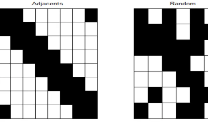
For the sake of exposition, suppose that firms have N = 8 departments and that there exist two schools, the Adjacent and the Random schools. Each school has its characteristic recommendation, the Adjacent school recommends that departments have to be linked with the departments that are adjacent, i.e. every firm link to 2 other departments, whereas the random school rec-ommends that departments have to be randomly linked to each other without any specification about the number of departments to which they are being connected.
Fig. 1. Example of school recomendations
For instance, considering that a black cell means ’to be linked with’, the rec-ommendation to the department number one from the Adjacent school is to link with department 2 and 85. On the other hand, the recommendation to the department number one coming from the Random school is to be link with department 3 and 5.
Thus, given the set of the strategies adopted by every department, {1, 0}, and the school recommendation that firms adopt, it is possible to compute the contribution of every department i to the firm.
Formally the fitness for a firm which adopts the recommendation σ and strategy s is given by f (σ, s) = 1 N N X i=1 c (σi, s) 5
where σi is the recommendation that the school σ gives to the department
i, s is the set of strategies that the all the departments within a firm made and c represents the contribution to the fitness that every department provides according to the recommendation σi.
The contribution table Ω is a list of 2N pseudo-random numbers uniformly distributed in (0, 1) . Thus, given the strategy selected by the departments and the set of links specified by the recommendation, the index p is computed with 1 < p < 2N. The function c uses the index to collect the corresponding pseudo-random number from the list Ω.
For the sake of exposition an example is developed. Suppose that a firm has N = 8 departments which have the strategies {1, 0, 0, 1, 0, 1, 0, 1} and that the firm adopt the recommendation σ. Moreover suppose that the recommendation for the department 2 is the following σ2 = {1, 2, 3}6. The index p in this case is
the decimal number that can be computed according to the current strategies of the departments 1, 2 and 3. This is p = (100)b = 4, where the notation
(.)b has been used to express that the number inside the brackets is binary. Thus the contribution of the department 2 is the pseudo-random number in the position 4 in the list Ω.
Up to now the configurational space XS and the fitness function fS have
been explained for the landscape of the firms, ΛS. Now it has to be explained
how firms move through the configurational space. In other words, according to the definition of landscape adopted, it is necessary to explain χs:
6Notice that this is the recomendation that the school Adjancents gives in figure 1, and
The set χs is composed by three evolutionary operators; selection, recombi-nation and mutation7.
Thus, the evolution explained in step 4 of the time-line simulations run as follows;
1. For every recommendation σ of a school, a fixed population of |S| firms with N departments is created. Besides, every department selects, ini-tially, a random strategy.
2. The fitness value of every firm in the |Σ| groups is computed according to the recommendation and the strategies adopted by the departments. 3. The operator of selection is applied to every population of firms,
obtain-ing |Σ| subsets of firms which have higher fitnesses within every popula-tion of firms.
4. In any population of firms, using the selected population of firms, the crossover operator is applied in order to obtain again the populations of |S| firms.
5. Over this new population the mutation operator is applied giving place to the new set of firms.
6. Go back to step 2 for τ periods.
Thus, for every school a firms using this genetic algorithm evolves through the configurational space.
7
Schools Landscape
During the description of the landscape of the firms ΛS, the school
recom-mendation has been explained.
Thus, we are able now to explain the configuration space in the schools landscape. Indeed assuming that firms have N departments and that schools have to produce recommendations about the link that every department has to have, the size of one school recommendation is N2.
Given that a recommendation specifies just whether one department is con-nected or not with the other departments, it is necessary that just 10s and 00s to specify this. Thus, the size of the space configuration XΣ for the school is 2N
2 . Notice that the configuration space for schools is bigger than the configuration space of the firms.
The fitness that one school σ obtains is computed as the mean of the fitness that firms that have been using its recommendations obtained. In other words,
f = 1 |S| |S| X j=1 Cj (1)
where |S| is the number of firms and Cj is the fitness that firm j obtains.
The schools move through the configuration space applying also the same evolutionary operators than firms use; selection, recombination and mutation. For the sake of clarity the sequence in the application of the operators is shown;
1. The initial population of |Σ| schools is created with their recommenda-tions randomly generated.
2. Firms evolve in their landscape and according to this, the fitness value of the schools is computed using 1.
3. Applying the operator of selection a proportion p of the best schools is obtained from the current Σ population.
4. Using the subpopulation obtained in step 3 and applying the operator of recombination the population of size |Σ| is recovered.
5. Over the new population of schools the mutation operator is applied. 6. Repeat step 2 to 5 during T periods.
COMPUTATIONAL COMPLEXITY
Given the specification of both landscapes ΛS and ΛΣ it is possible to be
more precise about the concept of complexity used in the paper.
Every recommendation produces a variation of the N K-Models proposed by Kauffman (2) in the landscape of firms, ΛS. Indeed in the case of the Adjacent
schools of figure 1, firms adopting its recommendation are searching through the N K model with adjacencies where N = 8 and K = 3.
As described by Kauffman (3), recommendations where K is low, i.e. few interrelationship among the departments, produce smooth landscapes that gave to firms greater chances of reaching the highest peak. On the other hand, when the value of K is close to N meaning that there is high interdependency among the departments and the change in one of them will impact all the other departments, the complexity of the space in which firms are searching for the
highest peak is greater.
The N K model has been studied using different configurations, (see (2), (3) and (6) for more details). Keeping the value of K fixed two main variation have been proposed; the adjacent and the random configurations. In the adjacent model the interrelationship of one department is with its K closer neighbors whereas in the random model one department is linked to K other departments randomly picked. Rugged landscapes will make the work of the optimizer harder.
The complexity in this paper is determined by the level of difficulties that firms have in finding out the optimal values in reality. The level of difficulty that a firm has in order to find out optimal values is given by the school recommendations. Notice that, as previously explained, a recommendation specifies the value of K for every department and the specific interrelationships between the departments.
It is possible to use some guides coming from the literature that give insights about the computational complexity of a reduced set of N K landscapes.
A landscape is assigned to the N P (nondeterministic polynomial time) class if it is verifiable in polynomial time by a nondeterministic Turing machine8.A P -problem, whose solution time is bounded by a polynomial, is always also N P . If a problem is known to be N P , and a solution to the problem is somehow known, then demonstrating the correctness of the solution can always 8A nondeterministc Turing machine is a parallel Turing machine which can take many
computational paths simultaneously, with the restriction that the parallel Turing machines cannot communicate.
be reduced to a single P (polynomial time) verification. If P and N P are not equivalent, then the solution of N P -problems requires (in the worst case) an exhaustive search. The P = N P , or, alternatively, P 6= NP , problem remains one of the great open problems in theoretical computer science.
The computational complexity of finding the optimum solution, i.e. the peak, in an N K landscape has been analyzed in the literature by (?) and (8). In any case the proofs developed depends on the structure of interrelation-ships. The main results can be summarized in the following four theorems,
Theorem 1 (Weinberger). The NK optimization problem with adjacent
neigh-borhoods is solvable in O¡2KN¢steps, and is thus in P .
Theorem 2 (Weinberger). The NK optimization problem with random
neigh-borhoods is N P complete for K ≥ 3.
Theorem 3 (Thompson and Wright). The NK optimization problem with
random K = 1 neighborhoods is solvable in polynomial time.
Theorem 4 (Thompson and Wright). The NK optimization problem with
random K = 2 is N P complete. Moreover, for a generalized K = 1 map with no requirement that mii = 19 for all i the N K optimization problem is N P
complete.
Under the hypothesis that system try to simplify the level of complexity, in order to obtain optimal values with less resources, the expected results as 9This requirement is equivalent to ask that department of firms includ themselve when
consequences of the model, is that the selected schools in Σ∗ will be the ones that recommend structures with adjacent neighborhoods. The idea is that N K landscapes with an adjacent structure produce P problems, which are simple to solve.
SIMULATIONS
The iterative model proposed is explored through computer simulations10. Every simulation has the following parameters; the populations are |Σ| = N and |S| = 2N.
Once a firm has a recommendation it applies the evolutive operators during τ = 200 periods in the search for optimal values in the reality Ω. On the other hand schools apply their evolutive operators during T = 100 periods.
The parameters of the genetic operators are the same for firms and schools11. The mutation rate is 0.001 and in every period 30% of the population is selected applying the roulette algorithm.
Monte Carlo experiments were ran for N = {10, 12, 14, 16, 18, 20}. For each value of N, 3 different realities Ω were generated, and keeping the same reality 10 simulations were run.
1 0
The code is in Matlab and the code of the program is available by request.
1 1
This parameters are the values where the evolutionary operators applied to N K models produce the best search.
Analysis
The focus of the analysis is the set of recommendations Σ∗ that remain at the end of the whole evolutionary process. Thus, in order to analyze this set for every recommendation σ ∈ Σ∗ three indexes are computed.
1. The mean level of links K that represent how tight are the departments between them. This index is computed according to
K = 1 N N X i=1 |σi|
where |σi| represent the number of links from i to other departments
that the recommendation σ proposes. The minimum number that |σi|
can assume is 1 because every department is linked to itself. On the other hand N is the maximum number of departments in a firm. Thus this index varies in the range 1 ≤ K ≤ N.
2. In order to capture how important is the variation within a recommen-dation for every department the coefficient of variation is computed as
v = v u u t1 N N X i=1 ¡ K − |σi| ¢2 K
3. The index of adjacency ϕ related to every recommendation gives infor-mation about the level of adjacency among the departments in every recommendation and it is computed as follows. Given that the recom-mendation σi to a department i is represented as a binary string, any
department included i, can have zero, one or two adjacent departments. Thus, the maximum number of adjacencies that can be present in a rec-ommendation σi is given by Ji∗ = ⎧ ⎨ ⎩ 2 (eσid − 1) if eσid < N 2 eσid if eσid = N
where eσid represents the number of ones that the recommendation to
the department i has. Thus, the mean index of adjacency of the recom-mendation σ is computed as12 ϕ = 1 N N X i=1 Ji J∗ i
where Ji∗ is the maximum number of adjacencies and Ji is the actual
number of adjacencies in σi.
For the sake of exposition the index of adjacency will be partially computed for one department. Suppose that the recommendation of the department 4 is σ4 = {1, 0, 1, 1, 0}, where N = 5. In this case J4∗ = 4 and J4 = 2. Notice that
department 1 does not have adjacencies. Department 3 and 4 have one each.
Simulation Results
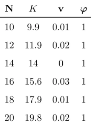
The mean of each of the three indexes over the 30 simulations are shown in Table 1 for every value of N.
The results obtained from the Monte Carlo experiments show two character-istics; first the result reinforce the prediction made about the complexity that
1 2
N K v ϕ 10 9.9 0.01 1 12 11.9 0.02 1 14 14 0 1 16 15.6 0.03 1 18 17.9 0.01 1 20 19.8 0.02 1
Table 1. Mean results of the simulations
the schools in Σ∗would recommend to the firms. Indeed the index of adjacency
shows that in any case the model selected is the adjacent one which represents a P problem. However, on the other hand, schools that succeed recommend to the firms the maximum degree of freedom that they could propose, which means that the level of interaction within a firm is maximum. This means that the schools recommend to the firms the most rugged landscape.
In other word, schools that survive are the one that leave the firms to do what they want to do. Indeed given that both algorithms have the same abilities to search, the coordination problem between schools and firms seems to introduce unnecessary noise in the search process. Thus, the best strategy that emerge is the one in which one of the algorithms becomes inactive and the other does its best.
CONCLUSIONS
The aim of this paper is to use a simple framework where problems with different levels of complexity can be selected to test which of this levels is chosen by agents using evolutionary features.
The simple framework is the Kauffman N K model; the level of complexity is given by the selection of the value of K and the structure of adjacency and the agents are represented by firms that select different recommendations, i.e. level of complexity, from schools. Firms and schools use evolutionary operators to search in their representation of reality.
The main result coming from the simulations shows that given that a search process is carried on by two algorithms with the same abilities to search, the coordination problem between both algorithms introduces unnecessary noise in the search process. Thus, the best strategy is that one of the algorithms become inactive such that the other can make its best.
On the other hand, this strategy of coordination between firms and school produces, in the framework of N K models the selection of rugged landscapes. This in turn, gives place to the existence of many firms using different strategies in the economy, because rugged landscape have many local optima, and firms will cluster around these local optima in their search for the highest peak.
REFERENCES
[1] Holm H. (2003). "Rights and Decentralized Computation". Metroeconomica, 2003.
[2] Kauffman, S. and S. Levin (1987). "Toward a General Theory of Adaptive Walks on Rugged Landscapes", Journal of Theoretical Biology, 128, 11-45, 1987.
[3] Kauffman, S. (1993). The Origin of Order, Oxford University Press, New York, 1993.
[4] Levinthal, Daniel (1997). "Adaptation on Rugged Landscapes". Management Science. Vol 43 No. 7, July 1997
[5] Rivkin J. and Siggelkow N., (2002). "Organizational Sticking Points on NK Landscapes". Complexity, Vol. 7, Nro. 5, 2002.
[6] Reidys, Christian and Stadler Peter (2002). "Combinatorial Landscapes". SIAM Review. Vol. 44 No. 1 pp 3-54.
[7] Scarf H. (1990). "Mathematical Programming and Economic Theory". Opera-tions Research, 38, pp 377-385.
[8] Thompson, R. and Wright. (1996). "Additively decomposable fitness functions". Technical Report. http://www.cs.umt.edu/CS/FAC/WRIGHT/pubs.htm [9] Weinberger E. "NP Completeness of Kauffman’s N-k Model, a Tuneably Rugged
Elenco dei papers del Dipartimento di Economia
1989. 1. Knowledge and Prediction of Economic Behaviour: Towards
A Constructivist Approach. by Roberto Tamborini.
1989. 2. Export Stabilization and Optimal Currency Baskets: the
Case of Latin American Countries. by Renzo G.Avesani Giampiero
M. Gallo and Peter Pauly.
1989. 3. Quali garanzie per i sottoscrittori di titoli di Stato? Una
rilettura del rapporto della Commissione Economica dell'Assemblea Costituente di Franco Spinelli e Danilo Vismara.
(What Guarantees to the Treasury Bill Holders? The Report of the
Assemblea Costituente Economic Commission Reconsidered by
Franco Spinelli and Danilo Vismara.)
1989. 4. L'intervento pubblico nell'economia della "Venezia
Tridentina" durante l'immediato dopoguerra di Angelo Moioli.
(The Public Intervention in "Venezia Tridentina" Economy in the
First War Aftermath by Angelo Moioli.)
1989. 5. L'economia lombarda verso la maturità dell'equilibrio
agricolo-commerciale durante l'età delle riforme di Angelo Moioli.
(The Lombard Economy Towards the Agriculture-Trade Equilibrium
in the Reform Age by Angelo Moioli.)
1989. 6. L'identificazione delle allocazioni dei fattori produttivi con il
duale. di Quirino Paris e di Luciano Pilati.
(Identification of Factor Allocations Through the Dual Approach by Quirino Paris and Luciano Pilati.)
1990. 1. Le scelte organizzative e localizzative dell'amministrazione
postale: un modello intrpretativo.di Gianfranco Cerea.
(The Post Service's Organizational and Locational Choices: An
Interpretative Model by Gianfranco Cerea.)
1990. 2. Towards a Consistent Characterization of the Financial
Economy. by Roberto Tamborini.
1990. 3. Nuova macroeconomia classica ed equilibrio economico
generale: considerazioni sulla pretesa matrice walrasiana della N.M.C. di Giuseppe Chirichiello.
(New Classical Macroeconomics and General Equilibrium: Some
Notes on the Alleged Walrasian Matrix of the N.C.M.by Giuseppe
Chirichiello.)
1990. 4. Exchange Rate Changes and Price Determination in
Polypolistic Markets. by Roberto Tamborini.
1990. 5. Congestione urbana e politiche del traffico. Un'analisi
economica di Giuseppe Folloni e Gianluigi Gorla.
(Urban Congestion and Traffic Policy. An Economic Analysis by Giuseppe Folloni and Gianluigi Gorla.)
1990. 6. Il ruolo della qualità nella domanda di servizi pubblici. Un
metodo di analisi empirica di Luigi Mittone.
(The Role of Quality in the Demand for Public Services. A
Methodology for Empirical Analysis by Luigi Mittone.)
1991. 1. Consumer Behaviour under Conditions of Incomplete
Information on Quality: a Note by Pilati Luciano and Giuseppe
Ricci.
1991. 2. Current Account and Budget Deficit in an Interdependent
World by Luigi Bosco.
1991. 3. Scelte di consumo, qualità incerta e razionalità limitata di Luigi Mittone e Roberto Tamborini.
(Consumer Choice, Unknown Quality and Bounded Rationality by Luigi Mittone and Roberto Tamborini.)
1991. 4. Jumping in the Band: Undeclared Intervention Thresholds in
a Target Zone by Renzo G. Avesani and Giampiero M. Gallo.
1991. 5 The World Tranfer Problem. Capital Flows and the
Adjustment of Payments by Roberto Tamborini.
1992.1 Can People Learn Rational Expectations? An Ecological
Approach by Pier Luigi Sacco.
1992.2 On Cash Dividends as a Social Institution by Luca Beltrametti.
(Pricing and Information Policy in the Supply of Public Services by Luigi Mittone.)
1992.4 Technological Change, Technological Systems, Factors of
Production by Gilberto Antonelli and Giovanni Pegoretti.
1992.5 Note in tema di progresso tecnico di Geremia Gios e Claudio Miglierina.
(Notes on Technical Progress, by Geremia Gios and Claudio Miglierina).
1992.6 Deflation in Input Output Tables by Giuseppe Folloni and Claudio Miglierina.
1992.7 Riduzione della complessità decisionale: politiche normative e
produzione di informazione di Luigi Mittone
(Reduction in decision complexity: normative policies and
information production by Luigi Mittone)
1992.8 Single Market Emu and Widening. Responses to Three
Institutional Shocks in the European Community by Pier Carlo
Padoan and Marcello Pericoli
1993.1 La tutela dei soggetti "privi di mezzi": Criteri e procedure per
la valutazione della condizione economica di Gianfranco Cerea
(Public policies for the poor: criteria and procedures for a novel means
test by Gianfranco Cerea )
1993.2 La tutela dei soggetti "privi di mezzi": un modello matematico
per la rappresentazione della condizione economica di Wolfgang J.
Irler
(Public policies for the poor: a mathematical model for a novel means
test by Wolfgang J.Irler)
1993.3 Quasi-markets and Uncertainty: the Case of General Proctice
Service by Luigi Mittone
1993.4 Aggregation of Individual Demand Functions and
Convergence to Walrasian Equilibria by Dario Paternoster
1993.5 A Learning Experiment with Classifier System: the
1993.6 Alcune considerazioni sui paesi a sviluppo recente di Silvio Goglio
(Latecomer Countries: Evidence and Comments by Silvio Goglio) 1993.7 Italia ed Europa: note sulla crisi dello SME di Luigi Bosco
( Italy and Europe: Notes on the Crisis of the EMS by Luigi Bosco) 1993.8 Un contributo all'analisi del mutamento strutturale nei
modelli input-output di Gabriella Berloffa
(Measuring Structural Change in Input-Output Models: a
Contribution by Gabriella Berloffa)
1993.9 On Competing Theories of Economic Growth: a Cross-country
Evidence by Maurizio Pugno
1993.10 Le obbligazioni comunali di Carlo Buratti (Municipal
Bonds by Carlo Buratti)
1993.11 Due saggi sull'organizzazione e il finanziamento della scuola
statale di Carlo Buratti
(Two Essays on the Organization and Financing of Italian State
Schools by Carlo Buratti
1994.1 Un'interpretazione della crescita regionale: leaders, attività
indotte e conseguenze di policy di Giuseppe Folloni e Silvio Giove.
(A Hypothesis about regional Growth: Leaders, induced Activities
and Policy by Giuseppe Folloni and Silvio Giove).
1994.2 Tax evasion and moral constraints: some experimental
evidence by Luigi Bosco and Luigi Mittone.
1995.1 A Kaldorian Model of Economic Growth with Shortage of
Labour and Innovations by Maurizio Pugno.
1995.2 A che punto è la storia d'impresa? Una riflessione
storiografica e due ricerche sul campo a cura di Luigi Trezzi.
1995.3 Il futuro dell'impresa cooperativa: tra sistemi, reti ed
ibridazioni di Luciano Pilati.
1995.4 Sulla possibile indeterminatezza di un sistema pensionistico in
perfetto equilibrio finanziario di Luca Beltrametti e Luigi Bonatti.
(On the indeterminacy of a perfectly balanced social security system by Luca Beltrametti and Luigi Bonatti).
1995.5 Two Goodwinian Models of Economic Growth for East Asian
NICs by Maurizio Pugno.
1995.6 Increasing Returns and Externalities: Introducing Spatial
Diffusion into Krugman's Economic Geography by Giuseppe
Folloni and Gianluigi Gorla.
1995.7 Benefit of Economic Policy Cooperation in a Model with
Current Account Dynamics and Budget Deficit by Luigi Bosco.
1995.8 Coalition and Cooperation in Interdependent Economies by Luigi Bosco.
1995.9 La finanza pubblica italiana e l'ingresso nell'unione monetaria
europea di Ferdinando Targetti.
(Italian Public Finance and the Entry in the EMU by Ferdinando Targetti)
1996.1 Employment, Growth and Income Inequality: some open
Questions by Annamaria Simonazzi and Paola Villa.
1996.2 Keynes' Idea of Uncertainty: a Proposal for its Quantification by Guido Fioretti.
1996.3 The Persistence of a "Low-Skill, Bad-Job Trap" in a Dynamic
Model of a Dual Labor Market by Luigi Bonatti.
1996.4 Lebanon: from Development to Civil War by Silvio Goglio.
1996.5 A Mediterranean Perspective on the Break-Down of the
Relationship between Participation and Fertility by Francesca Bettio
and Paola Villa.
1996.6 Is there any persistence in innovative activities? by Elena Cefis.
1997.1 Imprenditorialità nelle alpi fra età moderna e contemporanea a cura di Luigi Trezzi.
1997.2 Il costo del denaro è uno strumento anti-inflazionistico? di Roberto Tamborini.
(Is the Interest Rate an Anti-Inflationary Tool? by Roberto Tamborini).
1997.3 A Stability Pact for the EMU? by Roberto Tamborini.
1997.4 Mr Keynes and the Moderns by Axel Leijonhufvud.
1997.5 The Wicksellian Heritage by Axel Leijonhufvud. 1997.6 On pension policies in open economies by Luca Beltrametti and Luigi Bonatti.
1997.7 The Multi-Stakeholders Versus the Nonprofit Organisation by Carlo Borzaga and Luigi Mittone.
1997.8 How can the Choice of a Tme-Consistent Monetary Policy
have Systematic Real Effects? by Luigi Bonatti.
1997.9 Negative Externalities as the Cause of Growth in a
Neoclassical Model by Stefano Bartolini and Luigi Bonatti.
1997.10 Externalities and Growth in an Evolutionary Game by Angelo Antoci and Stefano Bartolini.
1997.11 An Investigation into the New Keynesian Macroeconomics of
Imperfect Capital Markets by Roberto Tamborini.
1998.1 Assessing Accuracy in Transition Probability Matrices by Elena Cefis and Giuseppe Espa.
1998.2 Microfoundations: Adaptative or Optimizing? by Axel Leijonhufvud.
1998.3 Clower’s intellectual voyage: the ‘Ariadne’s thread’ of
1998.4 The Persistence of Innovative Activities. A Cross-Countries
and Cross-Sectors Comparative Analysis by Elena Cefis and Luigi
Orsenigo
1998.5 Growth as a Coordination Failure by Stefano Bartolini and Luigi Bonatti
1998.6 Monetary Theory and Central Banking by Axel Leijonhufvud
1998.7 Monetary policy, credit and aggregate supply: the evidence
from Italy by Riccardo Fiorentini and Roberto Tamborini
1998.8 Stability and multiple equilibria in a model of talent, rent
seeking, and growth by Maurizio Pugno
1998.9 Two types of crisis by Axel Leijonhufvud
1998.10 Trade and labour markets: vertical and regional
differentiation in Italy by Giuseppe Celi e Maria Luigia Segnana
1998.11 Utilizzo della rete neurale nella costruzione di un trading
system by Giulio Pettenuzzo
1998.12 The impact of social security tax on the size of the informal
economy by Luigi Bonatti
1999.1 L’economia della montagna interna italiana: un approccio
storiografico, a cura di Andrea Leonardi e Andrea Bonoldi.
1999.2 Unemployment risk, labour force participation and savings, by Gabriella Berloffa e Peter Simmons
1999.3 Economia sommersa, disoccupazione e crescita, by Maurizio Pugno
1999.4 The nationalisation of the British Railways in Uruguay, by Giorgio Fodor
1999.5 Elements for the history of the standard commodity, by Giorgio Fodor
1999.6 Financial Market Imperfections, Heterogeneity and growth, by Edoardo Gaffeo
1999.7 Growth, real interest, employment and wage determination, by Luigi Bonatti
2000.1 A two-sector model of the effects of wage compression on
unemployment and industry distribution of employment, by Luigi
Bonatti
2000.2 From Kuwait to Kosovo: What have we learned? Reflections
on globalization and peace, by Roberto Tamborini
2000.3 Metodo e valutazione in economia. Dall’apriorismo a
Friedman , by Matteo Motterlini
2000.4 Under tertiarisation and unemployment. by Maurizio Pugno
2001.1 Growth and Monetary Rules in a Model with Competitive
Labor Markets, by Luigi Bonatti.
2001.2 Profit Versus Non-Profit Firms in the Service Sector: an
Analysis of the Employment and Welfare Implications, by Luigi
Bonatti, Carlo Borzaga and Luigi Mittone.
2001.3 Statistical Economic Approach to Mixed Stock-Flows
Dynamic Models in Macroeconomics, by Bernardo Maggi and
Giuseppe Espa.
2001.4 The monetary transmission mechanism in Italy: The credit
channel and a missing ring, by Riccardo Fiorentini and Roberto
Tamborini.
2001.5 Vat evasion: an experimental approach, by Luigi Mittone 2001.6 Decomposability and Modularity of Economic Interactions, by Luigi Marengo, Corrado Pasquali and Marco Valente.
2001.7 Unbalanced Growth and Women’s Homework, by Maurizio Pugno
2002.1 The Underground Economy and the Underdevelopment Trap, by Maria Rosaria Carillo and Maurizio Pugno.
2002.2 Interregional Income Redistribution and Convergence in a
Model with Perfect Capital Mobility and Unionized Labor Markets,
by Luigi Bonatti.
2002.3 Firms’ bankruptcy and turnover in a macroeconomy, by Marco Bee, Giuseppe Espa and Roberto Tamborini.
2002.4 One “monetary giant” with many “fiscal dwarfs”: the
efficiency of macroeconomic stabilization policies in the European Monetary Union, by Roberto Tamborini.
2002.5 The Boom that never was? Latin American Loans in London
1822-1825, by Giorgio Fodor.
2002.6 L’economia senza banditore di Axel Leijonhufvud: le ‘forze
oscure del tempo e dell’ignoranza’ e la complessità del coordinamento,
by Elisabetta De Antoni.
2002.7 Why is Trade between the European Union and the Transition Economies Vertical?, by Hubert Gabrisch and Maria
Luigia Segnana.
2003.1 The service paradox and endogenous economic gorwth, by Maurizio Pugno.
2003.2 Mappe di probabilità di sito archeologico: un passo avanti, di Giuseppe Espa, Roberto Benedetti, Anna De Meo e Salvatore Espa.
(Probability maps of archaeological site location: one step beyond, by Giuseppe Espa, Roberto Benedetti, Anna De Meo and Salvatore Espa).
2003.3 The Long Swings in Economic Understianding, by Axel Leijonhufvud.
2003.4 Dinamica strutturale e occupazione nei servizi, di Giulia Felice.