ScienceDirect
Available online at www.sciencedirect.com
Procedia Structural Integrity 24 (2019) 28–39
2452-3216 © 2019 The Authors. Published by Elsevier B.V.
This is an open access article under the CC BY-NC-ND license (http://creativecommons.org/licenses/by-nc-nd/4.0/) Peer-review under responsibility of the AIAS2019 organizers
10.1016/j.prostr.2020.02.003
10.1016/j.prostr.2020.02.003 2452-3216
© 2019 The Authors. Published by Elsevier B.V.
This is an open access article under the CC BY-NC-ND license (http://creativecommons.org/licenses/by-nc-nd/4.0/) Peer-review under responsibility of the AIAS2019 organizers
ScienceDirect
StructuralIntegrity Procedia 00 (2019) 000–000
www.elsevier.com/locate/procedia
2452-3216© 2019 The Authors. Published by Elsevier B.V.
This is an open access article under the CC BY-NC-ND license (http://creativecommons.org/licenses/by-nc-nd/4.0/) Peer-review under responsibility of the AIAS2019 organizers
AIAS 2019 International Conference on Stress Analysis
Two-Dimensional Discrete Model for Buckling of Helical Springs
Francesco De Crescenzo
a*, Pietro Salvini
aaDepartment of Enterpirese Engineering, University of Rome "Tor Vergata", via del Politecnico, 1 00133, Rome, Italy
Abstract
The classical theory of helical spring instability is based on the buckling of an equivalent column. Alternatively, more advanced methods are found in literature, involving the numerical solution of the displacement field of the helical wire. Those approaches turn challenging when the helix is non-uniform or there is the need to take into account contact between coils. In this work, the buckling behaviour of uniform helix springs is investigated using a 2D model with lumped stiffness, so that it can be compared to the previous modelling techniques. The aim is, after validation, to adopt the proposed technique to non-uniform springs. The spring is modelled as a planar structure made of rigid rods connected by nonlinear elastic hinges. Each rod thus represents half a coil, and each hinge lumps the stiffness of the adjacent two-quarters of a coil. Because of nonlinearity, the equilibrium is solved for incremental loads. At each step, the stability of the spring is evaluated from the eigenvalues of the tangent stiffness (geometric end elastic contributions).
© 2019 The Authors. Published by Elsevier B.V.
This is an open access article under the CC BY-NC-ND license (http://creativecommons.org/licenses/by-nc-nd/4.0/) Peer-review under responsibility of the AIAS2019 organizers
Keywords: Helical Springs; Nonlinear Buckling, Discrete modeling
* Corresponding author. Tel.: +39.06.7259.7140; fax: +39.06.7259.7140.
E-mail address: [email protected]
2 Francesco De Crescenzo and Pietro Salvini / StructuralIntegrity Procedia 00 (2019) 000–000
1. Introduction
1.1. Applications
The functionality of many mechanical systems depends on the capability of helical springs to absorb, store and release elastic energy. Just mentioning few examples, helical springs are key components in combustion engine distribution systems, vehicle suspensions, vibration insulating platforms, and in the actuation of safety mechanisms.
In all previous situations, helical springs are mostly loaded with an axial compressive force along their centreline, which may induce buckling if the spring is not properly designed. Moreover, axial loads lower the frequencies of lateral vibration modes, which may evidence unexpected resonances. In both cases, the spring may not operate at the design conditions anymore and this may compromise the performance, or even the integrity, of the whole system. The two phenomena, static instability and lowering of frequencies, are related and have often been studied together Kobelev (2014), Yildrim (2009).
Nomenclature
E Young's modulus of elasticity, N/m2 G shear modulus, N/m2
I moment of inertia of wire cross-section, m4 J polar moment of inertia of wire cross-section, m4 n number of coils
x generalized degree of freedom α helix angle, rad
ν Poisson's ratio 1.2. Haringx's model
The classical solution to the buckling of helical springs is that of Haringx (1948). He derived a simple model to predict instability, based on the buckling of an equivalent shearable column. The spring is modelled as an elastic column whose section properties depend on the deformed length in such a way that axial, bending, and shearing characteristics of the whole column are constant during compression. With this assumption, Haringx obtained a closed formula for buckling prediction, where the critical deflection of the spring is a function of spring slenderness only. This solution is very useful in early design stages and in good agreement with experimental results, especially when the number of coils is large, helix pitch is small and the wire is thin with respect to the coil radius. Haringx also showed the range of validity of his results giving an approximated solution of the elastica of the wire. He found the “auxiliary” helix that represents the deformed spring: this accounts for the effects of bending and torsion induced in the wire by the axial load. Finally, he considered small displacements and small rotations around the compressed state to check for instability.
1.3. Models based on helical wire elastica
In the following fifty years the problem was investigated by several authors, with the aim to obtain a better solution valid for springs not covered by Haringx model. The common approach recalls Haringx’s auxiliary helix and accounts of the differential equations governing the dynamics of the deformed wire. A numerical method is used for the search of eigenfrequencies, corresponding to a given axial load. Furthermore, the buckling condition (static response) corresponds to the load at 0 frequency, where the stiffness vanishes. The works differ for both the equation adopted (rotary inertia, shear deformation, prestress terms, …) and for the numerical method used to solve the system, which turns out to be made of 12 differential equations in 12 unknowns. Pearson (1982), Becker et al. (1992), Chassie et al. (1996) and Yildrim (2009) used Transfer Matrix Method (TMM); Mottershead (1982) also developed a helical Finite Element (FE).
Francesco De Crescenzo et al. / Procedia Structural Integrity 24 (2019) 28–39 29
ScienceDirect
StructuralIntegrity Procedia 00 (2019) 000–000
www.elsevier.com/locate/procedia
2452-3216© 2019 The Authors. Published by Elsevier B.V.
This is an open access article under the CC BY-NC-ND license (http://creativecommons.org/licenses/by-nc-nd/4.0/) Peer-review under responsibility of the AIAS2019 organizers
AIAS 2019 International Conference on Stress Analysis
Two-Dimensional Discrete Model for Buckling of Helical Springs
Francesco De Crescenzo
a*, Pietro Salvini
aaDepartment of Enterpirese Engineering, University of Rome "Tor Vergata", via del Politecnico, 1 00133, Rome, Italy
Abstract
The classical theory of helical spring instability is based on the buckling of an equivalent column. Alternatively, more advanced methods are found in literature, involving the numerical solution of the displacement field of the helical wire. Those approaches turn challenging when the helix is non-uniform or there is the need to take into account contact between coils. In this work, the buckling behaviour of uniform helix springs is investigated using a 2D model with lumped stiffness, so that it can be compared to the previous modelling techniques. The aim is, after validation, to adopt the proposed technique to non-uniform springs. The spring is modelled as a planar structure made of rigid rods connected by nonlinear elastic hinges. Each rod thus represents half a coil, and each hinge lumps the stiffness of the adjacent two-quarters of a coil. Because of nonlinearity, the equilibrium is solved for incremental loads. At each step, the stability of the spring is evaluated from the eigenvalues of the tangent stiffness (geometric end elastic contributions).
© 2019 The Authors. Published by Elsevier B.V.
This is an open access article under the CC BY-NC-ND license (http://creativecommons.org/licenses/by-nc-nd/4.0/) Peer-review under responsibility of the AIAS2019 organizers
Keywords: Helical Springs; Nonlinear Buckling, Discrete modeling
* Corresponding author. Tel.: +39.06.7259.7140; fax: +39.06.7259.7140.
E-mail address: [email protected]
2 Francesco De Crescenzo and Pietro Salvini / StructuralIntegrity Procedia 00 (2019) 000–000
1. Introduction
1.1. Applications
The functionality of many mechanical systems depends on the capability of helical springs to absorb, store and release elastic energy. Just mentioning few examples, helical springs are key components in combustion engine distribution systems, vehicle suspensions, vibration insulating platforms, and in the actuation of safety mechanisms.
In all previous situations, helical springs are mostly loaded with an axial compressive force along their centreline, which may induce buckling if the spring is not properly designed. Moreover, axial loads lower the frequencies of lateral vibration modes, which may evidence unexpected resonances. In both cases, the spring may not operate at the design conditions anymore and this may compromise the performance, or even the integrity, of the whole system. The two phenomena, static instability and lowering of frequencies, are related and have often been studied together Kobelev (2014), Yildrim (2009).
Nomenclature
E Young's modulus of elasticity, N/m2 G shear modulus, N/m2
I moment of inertia of wire cross-section, m4 J polar moment of inertia of wire cross-section, m4 n number of coils
x generalized degree of freedom α helix angle, rad
ν Poisson's ratio 1.2. Haringx's model
The classical solution to the buckling of helical springs is that of Haringx (1948). He derived a simple model to predict instability, based on the buckling of an equivalent shearable column. The spring is modelled as an elastic column whose section properties depend on the deformed length in such a way that axial, bending, and shearing characteristics of the whole column are constant during compression. With this assumption, Haringx obtained a closed formula for buckling prediction, where the critical deflection of the spring is a function of spring slenderness only. This solution is very useful in early design stages and in good agreement with experimental results, especially when the number of coils is large, helix pitch is small and the wire is thin with respect to the coil radius. Haringx also showed the range of validity of his results giving an approximated solution of the elastica of the wire. He found the “auxiliary” helix that represents the deformed spring: this accounts for the effects of bending and torsion induced in the wire by the axial load. Finally, he considered small displacements and small rotations around the compressed state to check for instability.
1.3. Models based on helical wire elastica
In the following fifty years the problem was investigated by several authors, with the aim to obtain a better solution valid for springs not covered by Haringx model. The common approach recalls Haringx’s auxiliary helix and accounts of the differential equations governing the dynamics of the deformed wire. A numerical method is used for the search of eigenfrequencies, corresponding to a given axial load. Furthermore, the buckling condition (static response) corresponds to the load at 0 frequency, where the stiffness vanishes. The works differ for both the equation adopted (rotary inertia, shear deformation, prestress terms, …) and for the numerical method used to solve the system, which turns out to be made of 12 differential equations in 12 unknowns. Pearson (1982), Becker et al. (1992), Chassie et al. (1996) and Yildrim (2009) used Transfer Matrix Method (TMM); Mottershead (1982) also developed a helical Finite Element (FE).
Both approaches are really effective. In particular, TMM gives the exact solution for a uniform helix at a very low computational cost. Mottershead's FE performs well and requires much coarser mesh than a standard FE analysis with beam elements. However, the effectiveness of those methods reduces when the helix is non-uniform since a more advanced formulation or a finer mesh is needed, Yildrim (1997). Furthermore, if coils clash and friction between the coils is to be taken into account, Wu et al. (1998), the implementation of TMM and helical FE methods becomes challenging. For this reason, the authors developed a 2D lumped model for helical springs buckling prediction, intending to extend it to non-uniform helices and to account possible coil contacts.
2. Model geometry and governing equations
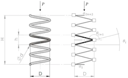
The proposed model is a planar structure made of rigid rods coupled by elastic hinges (Fig. 1).The rods are rigid and the stiffness of the hinges is deformation-dependent. Each elastic hinge lumps the stiffness of the adjacent two-quarter of a coil. The lumped model must have the same nonlinear axial load-deflection curve of the real spring. Moreover, to account for coil shearing, a linear spring is placed between the ends of adjacent rods, oriented along the bisector of the corresponding angle. Thus, each square in Fig.1 reacts with a torque to variation in relative angle between the rods, and with a sliding force against relative translations along angle bisector. First rod (link 1) and the last one (link 2𝑛𝑛 + 2) are dummy but needed to represent the clamped condition at helix ends.
Fig. 1. General representation of helical spring and its corresponding 2D discrete model.
The configuration of the links is given by the vector of rotations 𝜽𝜽 = {𝜃𝜃1, 𝜃𝜃2, … , 𝜃𝜃2𝑛𝑛+2}𝑇𝑇 and the vector of
translations 𝒖𝒖 = {𝑢𝑢1, 𝑢𝑢2, … , 𝑢𝑢2𝑛𝑛+1}𝑇𝑇, where 𝑛𝑛 is the number of coils. The total number of degrees of freedom is thus
4𝑛𝑛 + 3. 𝜃𝜃𝑖𝑖 represents the angle of rod 𝑖𝑖 with respect to the horizontal line, 𝑢𝑢𝑖𝑖 represents the translation of rod 𝑖𝑖 +
1 with respect to rod 𝑖𝑖. It follows that the total height of the spring is: 𝐻𝐻 = ∑ 𝑎𝑎𝑖𝑖sin 𝜃𝜃𝑖𝑖 2𝑛𝑛+2 𝑖𝑖=1 + ∑ 𝑢𝑢𝑘𝑘sin 𝑏𝑏𝑘𝑘 2𝑛𝑛+1 𝑘𝑘=1 (1) where 𝑎𝑎𝑖𝑖 is the length of the rod and 𝑏𝑏𝑘𝑘is the angle of the bisector with respect to the horizontal line:
𝑏𝑏𝑘𝑘=𝜃𝜃𝑖𝑖+ 𝜃𝜃2 𝑖𝑖+1−𝜋𝜋2 (2)
The potential of the load 𝑃𝑃 compressing the spring is:
𝑉𝑉𝑃𝑃= 𝑃𝑃𝑃𝑃 = 𝑃𝑃 ( ∑ 𝑎𝑎𝑖𝑖sin 𝜃𝜃𝑖𝑖 2𝑛𝑛+2 𝑖𝑖=1 + ∑ 𝑢𝑢𝑘𝑘sin 𝑏𝑏𝑘𝑘 2𝑛𝑛+1 𝑘𝑘=1 ) (3) At any equilibrium point 𝐱𝐱𝟎𝟎= {𝜽𝜽𝟎𝟎, 𝒖𝒖𝟎𝟎}𝑇𝑇 the sum of elastic and load potential is stationary; thus, 𝑔𝑔𝑔𝑔𝑎𝑎𝑔𝑔(𝑉𝑉𝐸𝐸+
𝑉𝑉𝑃𝑃) = 𝟎𝟎. This leads to the 2𝑛𝑛 + 2 equations describing the rotational equilibrium of the 𝑖𝑖𝑡𝑡ℎ rods and to 2𝑛𝑛 + 1
equations for the shearing of 𝑘𝑘𝑡𝑡ℎ linear spring:
𝜕𝜕𝑉𝑉𝐸𝐸 𝜕𝜕𝜃𝜃𝑖𝑖+ 𝜕𝜕𝑉𝑉𝑃𝑃 𝜕𝜕𝜃𝜃𝑖𝑖 = 0 𝑖𝑖 = 1, . . . ,2𝑛𝑛 + 2 (4) 𝜕𝜕𝑉𝑉𝐸𝐸 𝜕𝜕𝑢𝑢𝑘𝑘+ 𝜕𝜕𝑉𝑉𝑃𝑃 𝜕𝜕𝑢𝑢𝑘𝑘= 0 𝑘𝑘 = 1, . . . ,2𝑛𝑛 + 1 (5)
If an incremental load Δ𝑃𝑃 is applied to the structure, the gradient of corresponding potential 𝑉𝑉𝑃𝑃+Δ𝑃𝑃 will not be
balanced by the elastic forces anymore, however it is still reasonable to look for equilibrium point near 𝒙𝒙𝟎𝟎
expanding terms in the previous equations: 𝜕𝜕𝑉𝑉𝐸𝐸 𝜕𝜕𝑥𝑥𝑖𝑖 |𝒙𝒙=𝒙𝒙𝟎𝟎+ ∑ 𝜕𝜕2𝑉𝑉 𝐸𝐸 𝜕𝜕𝑥𝑥𝑗𝑗𝜕𝜕𝑥𝑥𝑖𝑖|𝒙𝒙=𝒙𝒙𝟎𝟎Δ𝑥𝑥𝑗𝑗 4𝑛𝑛+3 𝑗𝑗=1 +𝜕𝜕𝑉𝑉𝜕𝜕𝑥𝑥𝑃𝑃 𝑖𝑖 |𝒙𝒙=𝒙𝒙𝟎𝟎 + ∑ 𝜕𝜕𝑥𝑥𝜕𝜕2𝑉𝑉𝑃𝑃 𝑗𝑗𝜕𝜕𝑥𝑥𝑖𝑖|𝒙𝒙=𝒙𝒙𝟎𝟎Δ𝑥𝑥𝑗𝑗 4𝑛𝑛+3 𝑗𝑗=1 +𝜕𝜕𝑉𝑉𝜕𝜕𝑥𝑥Δ𝑃𝑃 𝑖𝑖 |𝒙𝒙=𝒙𝒙𝟎𝟎 = 0 𝑖𝑖 = 1,2, . . .4𝑛𝑛 + 3 (6) On the assumption that 𝒙𝒙𝟎𝟎was an equilibrium point associated to load 𝑃𝑃, it gives:
∑ 𝜕𝜕2𝑉𝑉𝐸𝐸 𝜕𝜕𝑥𝑥𝑗𝑗𝜕𝜕𝑥𝑥𝑖𝑖Δ𝑥𝑥𝑗𝑗 4𝑛𝑛+3 𝑗𝑗=1 + ∑ 𝜕𝜕2𝑉𝑉𝑃𝑃 𝜕𝜕𝑥𝑥𝑗𝑗𝜕𝜕𝑥𝑥𝑖𝑖Δ𝑥𝑥𝑗𝑗 4𝑛𝑛+3 𝑗𝑗=1 +𝜕𝜕𝑉𝑉Δ𝑃𝑃 𝜕𝜕𝑥𝑥𝑖𝑖 = 0 𝑖𝑖 = 1,2, . . .4𝑛𝑛 + 3 (7)
Eq.(7) can be written in matrix form as:
(𝑲𝑲𝑒𝑒+ 𝑲𝑲𝑔𝑔)𝚫𝚫𝒙𝒙 = 𝚫𝚫𝑭𝑭 (8)
where the sum (𝑲𝑲𝑒𝑒+ 𝑲𝑲𝑔𝑔) is the tangent stiffness, considering elastic and geometric contributions, 𝚫𝚫𝑭𝑭 is the vector
of external loads increment and 𝚫𝚫𝒙𝒙 is the corresponding incremental displacement. Since eq.(8) is only a linear approximation of the incremental equilibrium, an iterative procedure must be implemented in order to find a solution within a prescribed tolerance.
3. Derivation of stiffness parameters
3.1. Load potential and geometric stiffness matrix
Geometric stiffness terms are obtained performing the second partial derivative of load potential in eq.(3). For easiness of writing, in the following the numbering of the degrees of freedom starts from 0 , (𝑏𝑏0, 𝑢𝑢0, 𝑏𝑏2𝑛𝑛+2, 𝑢𝑢2𝑛𝑛+2) ≡
0; thus avoiding the need of explicitly writing the expressions involving first and last rods. It is useful to separate the contribution of pure rotation, pure shearing and rotation-shearing coupling terms.
Derivation of terms in the rotation-to-rotation geometric stiffness block 𝜃𝜃𝜃𝜃𝐾𝐾
𝑔𝑔𝑖𝑖𝑖𝑖 is straightforward. Starting from the potential, the calculation of the second derivatives gives:
𝜃𝜃𝜃𝜃𝐾𝐾 𝑔𝑔𝑖𝑖𝑖𝑖= 𝜕𝜕2𝑉𝑉 𝑃𝑃 𝜕𝜕𝜃𝜃𝑗𝑗𝜕𝜕𝜃𝜃𝑖𝑖= 𝑃𝑃 (−𝑎𝑎𝑖𝑖sin 𝜃𝜃𝑗𝑗− 1 4𝑢𝑢𝑖𝑖−1sin 𝑏𝑏𝑗𝑗−1− 1 4𝑢𝑢𝑖𝑖sin 𝑏𝑏𝑗𝑗) 𝛿𝛿𝑖𝑖𝑗𝑗 (9)
Both approaches are really effective. In particular, TMM gives the exact solution for a uniform helix at a very low computational cost. Mottershead's FE performs well and requires much coarser mesh than a standard FE analysis with beam elements. However, the effectiveness of those methods reduces when the helix is non-uniform since a more advanced formulation or a finer mesh is needed, Yildrim (1997). Furthermore, if coils clash and friction between the coils is to be taken into account, Wu et al. (1998), the implementation of TMM and helical FE methods becomes challenging. For this reason, the authors developed a 2D lumped model for helical springs buckling prediction, intending to extend it to non-uniform helices and to account possible coil contacts.
2. Model geometry and governing equations
The proposed model is a planar structure made of rigid rods coupled by elastic hinges (Fig. 1).The rods are rigid and the stiffness of the hinges is deformation-dependent. Each elastic hinge lumps the stiffness of the adjacent two-quarter of a coil. The lumped model must have the same nonlinear axial load-deflection curve of the real spring. Moreover, to account for coil shearing, a linear spring is placed between the ends of adjacent rods, oriented along the bisector of the corresponding angle. Thus, each square in Fig.1 reacts with a torque to variation in relative angle between the rods, and with a sliding force against relative translations along angle bisector. First rod (link 1) and the last one (link 2𝑛𝑛 + 2) are dummy but needed to represent the clamped condition at helix ends.
Fig. 1. General representation of helical spring and its corresponding 2D discrete model.
The configuration of the links is given by the vector of rotations 𝜽𝜽 = {𝜃𝜃1, 𝜃𝜃2, … , 𝜃𝜃2𝑛𝑛+2}𝑇𝑇 and the vector of
translations 𝒖𝒖 = {𝑢𝑢1, 𝑢𝑢2, … , 𝑢𝑢2𝑛𝑛+1}𝑇𝑇, where 𝑛𝑛 is the number of coils. The total number of degrees of freedom is thus
4𝑛𝑛 + 3. 𝜃𝜃𝑖𝑖 represents the angle of rod 𝑖𝑖 with respect to the horizontal line, 𝑢𝑢𝑖𝑖 represents the translation of rod 𝑖𝑖 +
1 with respect to rod 𝑖𝑖. It follows that the total height of the spring is: 𝐻𝐻 = ∑ 𝑎𝑎𝑖𝑖sin 𝜃𝜃𝑖𝑖 2𝑛𝑛+2 𝑖𝑖=1 + ∑ 𝑢𝑢𝑘𝑘sin 𝑏𝑏𝑘𝑘 2𝑛𝑛+1 𝑘𝑘=1 (1) where 𝑎𝑎𝑖𝑖 is the length of the rod and 𝑏𝑏𝑘𝑘is the angle of the bisector with respect to the horizontal line:
𝑏𝑏𝑘𝑘 =𝜃𝜃𝑖𝑖+ 𝜃𝜃2 𝑖𝑖+1−𝜋𝜋2 (2)
The potential of the load 𝑃𝑃 compressing the spring is:
𝑉𝑉𝑃𝑃= 𝑃𝑃𝑃𝑃 = 𝑃𝑃 ( ∑ 𝑎𝑎𝑖𝑖sin 𝜃𝜃𝑖𝑖 2𝑛𝑛+2 𝑖𝑖=1 + ∑ 𝑢𝑢𝑘𝑘sin 𝑏𝑏𝑘𝑘 2𝑛𝑛+1 𝑘𝑘=1 ) (3) At any equilibrium point 𝐱𝐱𝟎𝟎= {𝜽𝜽𝟎𝟎, 𝒖𝒖𝟎𝟎}𝑇𝑇 the sum of elastic and load potential is stationary; thus, 𝑔𝑔𝑔𝑔𝑎𝑎𝑔𝑔(𝑉𝑉𝐸𝐸+
𝑉𝑉𝑃𝑃) = 𝟎𝟎. This leads to the 2𝑛𝑛 + 2 equations describing the rotational equilibrium of the 𝑖𝑖𝑡𝑡ℎ rods and to 2𝑛𝑛 + 1
equations for the shearing of 𝑘𝑘𝑡𝑡ℎ linear spring:
𝜕𝜕𝑉𝑉𝐸𝐸 𝜕𝜕𝜃𝜃𝑖𝑖 + 𝜕𝜕𝑉𝑉𝑃𝑃 𝜕𝜕𝜃𝜃𝑖𝑖 = 0 𝑖𝑖 = 1, . . . ,2𝑛𝑛 + 2 (4) 𝜕𝜕𝑉𝑉𝐸𝐸 𝜕𝜕𝑢𝑢𝑘𝑘+ 𝜕𝜕𝑉𝑉𝑃𝑃 𝜕𝜕𝑢𝑢𝑘𝑘 = 0 𝑘𝑘 = 1, . . . ,2𝑛𝑛 + 1 (5)
If an incremental load Δ𝑃𝑃 is applied to the structure, the gradient of corresponding potential 𝑉𝑉𝑃𝑃+Δ𝑃𝑃 will not be
balanced by the elastic forces anymore, however it is still reasonable to look for equilibrium point near 𝒙𝒙𝟎𝟎
expanding terms in the previous equations: 𝜕𝜕𝑉𝑉𝐸𝐸 𝜕𝜕𝑥𝑥𝑖𝑖 |𝒙𝒙=𝒙𝒙𝟎𝟎+ ∑ 𝜕𝜕2𝑉𝑉 𝐸𝐸 𝜕𝜕𝑥𝑥𝑗𝑗𝜕𝜕𝑥𝑥𝑖𝑖|𝒙𝒙=𝒙𝒙𝟎𝟎Δ𝑥𝑥𝑗𝑗 4𝑛𝑛+3 𝑗𝑗=1 +𝜕𝜕𝑉𝑉𝜕𝜕𝑥𝑥𝑃𝑃 𝑖𝑖 |𝒙𝒙=𝒙𝒙𝟎𝟎 + ∑ 𝜕𝜕𝑥𝑥𝜕𝜕2𝑉𝑉𝑃𝑃 𝑗𝑗𝜕𝜕𝑥𝑥𝑖𝑖|𝒙𝒙=𝒙𝒙𝟎𝟎Δ𝑥𝑥𝑗𝑗 4𝑛𝑛+3 𝑗𝑗=1 +𝜕𝜕𝑉𝑉𝜕𝜕𝑥𝑥Δ𝑃𝑃 𝑖𝑖 |𝒙𝒙=𝒙𝒙𝟎𝟎 = 0 𝑖𝑖 = 1,2, . . .4𝑛𝑛 + 3 (6) On the assumption that 𝒙𝒙𝟎𝟎was an equilibrium point associated to load 𝑃𝑃, it gives:
∑ 𝜕𝜕2𝑉𝑉𝐸𝐸 𝜕𝜕𝑥𝑥𝑗𝑗𝜕𝜕𝑥𝑥𝑖𝑖Δ𝑥𝑥𝑗𝑗 4𝑛𝑛+3 𝑗𝑗=1 + ∑ 𝜕𝜕2𝑉𝑉𝑃𝑃 𝜕𝜕𝑥𝑥𝑗𝑗𝜕𝜕𝑥𝑥𝑖𝑖Δ𝑥𝑥𝑗𝑗 4𝑛𝑛+3 𝑗𝑗=1 +𝜕𝜕𝑉𝑉Δ𝑃𝑃 𝜕𝜕𝑥𝑥𝑖𝑖 = 0 𝑖𝑖 = 1,2, . . .4𝑛𝑛 + 3 (7)
Eq.(7) can be written in matrix form as:
(𝑲𝑲𝑒𝑒+ 𝑲𝑲𝑔𝑔)𝚫𝚫𝒙𝒙 = 𝚫𝚫𝑭𝑭 (8)
where the sum (𝑲𝑲𝑒𝑒+ 𝑲𝑲𝑔𝑔) is the tangent stiffness, considering elastic and geometric contributions, 𝚫𝚫𝑭𝑭 is the vector
of external loads increment and 𝚫𝚫𝒙𝒙 is the corresponding incremental displacement. Since eq.(8) is only a linear approximation of the incremental equilibrium, an iterative procedure must be implemented in order to find a solution within a prescribed tolerance.
3. Derivation of stiffness parameters
3.1. Load potential and geometric stiffness matrix
Geometric stiffness terms are obtained performing the second partial derivative of load potential in eq.(3). For easiness of writing, in the following the numbering of the degrees of freedom starts from 0 , (𝑏𝑏0, 𝑢𝑢0, 𝑏𝑏2𝑛𝑛+2, 𝑢𝑢2𝑛𝑛+2) ≡
0; thus avoiding the need of explicitly writing the expressions involving first and last rods. It is useful to separate the contribution of pure rotation, pure shearing and rotation-shearing coupling terms.
Derivation of terms in the rotation-to-rotation geometric stiffness block 𝜃𝜃𝜃𝜃𝐾𝐾
𝑔𝑔𝑖𝑖𝑖𝑖 is straightforward. Starting from the potential, the calculation of the second derivatives gives:
𝜃𝜃𝜃𝜃𝐾𝐾 𝑔𝑔𝑖𝑖𝑖𝑖= 𝜕𝜕2𝑉𝑉 𝑃𝑃 𝜕𝜕𝜃𝜃𝑗𝑗𝜕𝜕𝜃𝜃𝑖𝑖= 𝑃𝑃 (−𝑎𝑎𝑖𝑖sin 𝜃𝜃𝑗𝑗− 1 4𝑢𝑢𝑖𝑖−1sin 𝑏𝑏𝑗𝑗−1− 1 4𝑢𝑢𝑖𝑖sin 𝑏𝑏𝑗𝑗) 𝛿𝛿𝑖𝑖𝑗𝑗 (9)
where 𝛿𝛿𝑖𝑖𝑖𝑖 is the Kronecker delta, thus 𝜃𝜃𝜃𝜃𝐾𝐾𝑔𝑔𝑖𝑖𝑖𝑖is a diagonal matrix.
Rotation and shearing are coupled, in fact the shearing effect of the load depends on the bisectors, which are a function of the angles of adjacent rods. Non-zero terms are of the rotation-to-shearing block are:
𝜃𝜃𝜃𝜃𝐾𝐾 𝑔𝑔𝑖𝑖𝑖𝑖 = 𝜕𝜕2𝑉𝑉 𝑃𝑃 𝜕𝜕𝑢𝑢𝑘𝑘𝜕𝜕𝜃𝜃𝑖𝑖= 1 2 𝑃𝑃 cos 𝑏𝑏𝑘𝑘= 𝜃𝜃𝜃𝜃𝐾𝐾𝑔𝑔𝑖𝑖𝑖𝑖 (10) with 𝑘𝑘 = 𝑖𝑖 − 1 𝑎𝑎𝑎𝑎𝑎𝑎 𝑖𝑖, considering 𝑘𝑘 ≠ 0.
As the load is vertical, there is no pure shearing geometric effect:
𝜃𝜃𝜃𝜃𝐾𝐾 𝑔𝑔𝑖𝑖𝑖𝑖 = 𝜕𝜕2𝑉𝑉 𝑃𝑃+Δ𝑃𝑃 𝜕𝜕𝑢𝑢𝑖𝑖𝜕𝜕𝑢𝑢𝑘𝑘 = 0 (11) for all 𝑘𝑘, 𝑗𝑗.
Ordering the degrees of freedom the complete geometric stiffness is obtained: 𝑲𝑲𝒈𝒈= [
𝜽𝜽𝜽𝜽𝑲𝑲
𝒈𝒈 𝜽𝜽𝜽𝜽𝑲𝑲𝒈𝒈 𝜽𝜽𝜽𝜽𝑲𝑲
𝒈𝒈 𝜽𝜽𝜽𝜽𝑲𝑲𝒈𝒈 ] (12)
3.2. Elastic deformation energy
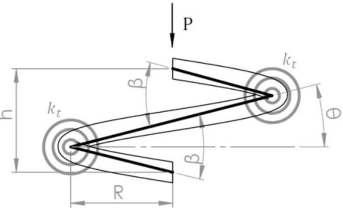
Elastic stiffness can be computed from the increment of elastic energy in a single coil under compression, as shown in Fig. 2. The fundamental assumptions are the followings:
each hinge lumps the stiffness of a two-quarters of a coil
two-quarter-coil compression is related to the angle between adjacent links
When the compression increases of an infinitesimal 𝑎𝑎ℎ, the corresponding increment of elastic energy is Δ𝐸𝐸𝐻𝐻=12𝐾𝐾𝐻𝐻𝑎𝑎ℎ2 (13)
where 𝐾𝐾𝐻𝐻 is the tangent stiffness of the coil, and will be derived in the next section. In the 2D lumped coil, the
elastic energy is stored by the two torsion springs 𝑘𝑘𝑡𝑡 subjected to angular deflection 𝑎𝑎β:
Δ𝐸𝐸𝑡𝑡= 212𝑘𝑘𝑡𝑡𝑎𝑎𝛽𝛽2 (14)
The kinematic constraint is:
𝑎𝑎ℎ = 2𝑎𝑎 cos 𝜃𝜃 𝑎𝑎𝜃𝜃 (15) where 𝑎𝑎𝜃𝜃 is the variation in rod slope and 𝑎𝑎𝛽𝛽 = 2𝑎𝑎𝜃𝜃 for symmetry. The value of 𝐾𝐾𝑡𝑡 is found by equating the energy
of the 2D model to that of the coil:
Δ𝐸𝐸𝐻𝐻=12 𝐾𝐾𝐻𝐻(2𝑎𝑎 cos 𝜃𝜃 𝑎𝑎𝜃𝜃)2= 𝑘𝑘𝑡𝑡(2𝑎𝑎𝜃𝜃)2= Δ𝐸𝐸𝑡𝑡 (16)
Fig. 2. Two springs, each one lumping two-quarters of a coil.
which gives:
𝑘𝑘𝑡𝑡=12𝐾𝐾𝐻𝐻𝑎𝑎2cos 𝜃𝜃2 (17)
3.3. Load-deflection characteristics of single coil
Axial force/deflection characteristics are derived following Wahl (1963). Shear and axial deformability of the wires are neglected, thus variation in radius and pitch can be related to wire curvature and torsion. Curvature and torsion of a cylindrical helix with radius 𝑅𝑅 and angle 𝛼𝛼 are:
𝜅𝜅 =cos𝑅𝑅 (18)2𝛼𝛼 𝜏𝜏 =cos 𝛼𝛼 sin 𝛼𝛼𝑅𝑅 (19)
For large spring index (𝐶𝐶 =𝐷𝐷𝑑𝑑≫ 1) bending and torsional moments can be related to the change in curvature and torsion Wahl (1963): 𝑀𝑀𝑏𝑏 = 𝐸𝐸𝐸𝐸 (cos 2𝛼𝛼 𝑅𝑅 − cos2𝛼𝛼 0 𝑅𝑅0 ) (20)
𝑀𝑀𝑡𝑡= 𝐺𝐺𝐺𝐺 (cos 𝛼𝛼 sin 𝛼𝛼𝑅𝑅 −cos 𝛼𝛼𝑅𝑅0sin 𝛼𝛼0
0 ) (21)
Bending and torsion moments due to an axial load acting along helix centreline are:
𝑀𝑀𝑏𝑏= 𝑃𝑃𝑅𝑅 sin 𝛼𝛼 (22)
𝑀𝑀𝑡𝑡= 𝑃𝑃𝑅𝑅 cos 𝛼𝛼 (23)
Furthermore, the wire is inextensible and total length is preserved: 𝑛𝑛cos 𝛼𝛼 = 𝑛𝑛2𝜋𝜋𝑅𝑅 0cos 𝛼𝛼2𝜋𝜋𝑅𝑅0
where 𝛿𝛿𝑖𝑖𝑖𝑖 is the Kronecker delta, thus 𝜃𝜃𝜃𝜃𝐾𝐾𝑔𝑔𝑖𝑖𝑖𝑖is a diagonal matrix.
Rotation and shearing are coupled, in fact the shearing effect of the load depends on the bisectors, which are a function of the angles of adjacent rods. Non-zero terms are of the rotation-to-shearing block are:
𝜃𝜃𝜃𝜃𝐾𝐾 𝑔𝑔𝑖𝑖𝑖𝑖= 𝜕𝜕2𝑉𝑉 𝑃𝑃 𝜕𝜕𝑢𝑢𝑘𝑘𝜕𝜕𝜃𝜃𝑖𝑖= 1 2 𝑃𝑃 cos 𝑏𝑏𝑘𝑘 = 𝜃𝜃𝜃𝜃𝐾𝐾𝑔𝑔𝑖𝑖𝑖𝑖 (10) with 𝑘𝑘 = 𝑖𝑖 − 1 𝑎𝑎𝑎𝑎𝑎𝑎 𝑖𝑖, considering 𝑘𝑘 ≠ 0.
As the load is vertical, there is no pure shearing geometric effect:
𝜃𝜃𝜃𝜃𝐾𝐾 𝑔𝑔𝑖𝑖𝑖𝑖= 𝜕𝜕2𝑉𝑉 𝑃𝑃+Δ𝑃𝑃 𝜕𝜕𝑢𝑢𝑖𝑖𝜕𝜕𝑢𝑢𝑘𝑘 = 0 (11) for all 𝑘𝑘, 𝑗𝑗.
Ordering the degrees of freedom the complete geometric stiffness is obtained: 𝑲𝑲𝒈𝒈= [
𝜽𝜽𝜽𝜽𝑲𝑲
𝒈𝒈 𝜽𝜽𝜽𝜽𝑲𝑲𝒈𝒈 𝜽𝜽𝜽𝜽𝑲𝑲
𝒈𝒈 𝜽𝜽𝜽𝜽𝑲𝑲𝒈𝒈 ] (12)
3.2. Elastic deformation energy
Elastic stiffness can be computed from the increment of elastic energy in a single coil under compression, as shown in Fig. 2. The fundamental assumptions are the followings:
each hinge lumps the stiffness of a two-quarters of a coil
two-quarter-coil compression is related to the angle between adjacent links
When the compression increases of an infinitesimal 𝑎𝑎ℎ, the corresponding increment of elastic energy is Δ𝐸𝐸𝐻𝐻 =12𝐾𝐾𝐻𝐻𝑎𝑎ℎ2 (13)
where 𝐾𝐾𝐻𝐻 is the tangent stiffness of the coil, and will be derived in the next section. In the 2D lumped coil, the
elastic energy is stored by the two torsion springs 𝑘𝑘𝑡𝑡 subjected to angular deflection 𝑎𝑎β:
Δ𝐸𝐸𝑡𝑡= 212𝑘𝑘𝑡𝑡𝑎𝑎𝛽𝛽2 (14)
The kinematic constraint is:
𝑎𝑎ℎ = 2𝑎𝑎 cos 𝜃𝜃 𝑎𝑎𝜃𝜃 (15) where 𝑎𝑎𝜃𝜃 is the variation in rod slope and 𝑎𝑎𝛽𝛽 = 2𝑎𝑎𝜃𝜃 for symmetry. The value of 𝐾𝐾𝑡𝑡 is found by equating the energy
of the 2D model to that of the coil:
Δ𝐸𝐸𝐻𝐻=12 𝐾𝐾𝐻𝐻(2𝑎𝑎 cos 𝜃𝜃 𝑎𝑎𝜃𝜃)2= 𝑘𝑘𝑡𝑡(2𝑎𝑎𝜃𝜃)2= Δ𝐸𝐸𝑡𝑡 (16)
Fig. 2. Two springs, each one lumping two-quarters of a coil.
which gives:
𝑘𝑘𝑡𝑡=12𝐾𝐾𝐻𝐻𝑎𝑎2cos 𝜃𝜃2 (17)
3.3. Load-deflection characteristics of single coil
Axial force/deflection characteristics are derived following Wahl (1963). Shear and axial deformability of the wires are neglected, thus variation in radius and pitch can be related to wire curvature and torsion. Curvature and torsion of a cylindrical helix with radius 𝑅𝑅 and angle 𝛼𝛼 are:
𝜅𝜅 =cos𝑅𝑅 (18)2𝛼𝛼 𝜏𝜏 =cos 𝛼𝛼 sin 𝛼𝛼𝑅𝑅 (19)
For large spring index (𝐶𝐶 =𝐷𝐷𝑑𝑑≫ 1) bending and torsional moments can be related to the change in curvature and torsion Wahl (1963): 𝑀𝑀𝑏𝑏= 𝐸𝐸𝐸𝐸 (cos 2𝛼𝛼 𝑅𝑅 − cos2𝛼𝛼 0 𝑅𝑅0 ) (20)
𝑀𝑀𝑡𝑡= 𝐺𝐺𝐺𝐺 (cos 𝛼𝛼 sin 𝛼𝛼𝑅𝑅 −cos 𝛼𝛼𝑅𝑅0sin 𝛼𝛼0
0 ) (21)
Bending and torsion moments due to an axial load acting along helix centreline are:
𝑀𝑀𝑏𝑏 = 𝑃𝑃𝑅𝑅 sin 𝛼𝛼 (22)
𝑀𝑀𝑡𝑡= 𝑃𝑃𝑅𝑅 cos 𝛼𝛼 (23)
Furthermore, the wire is inextensible and total length is preserved: 𝑛𝑛cos 𝛼𝛼2𝜋𝜋𝑅𝑅 = 𝑛𝑛0cos 𝛼𝛼2𝜋𝜋𝑅𝑅0
It is convenient to assign a value to the helix angle and then to compute the corresponding radius and load. By this way, it is possible to table loads against deflection and to compute the tangent characteristic of the coil using central difference
𝑅𝑅 = 𝑅𝑅0[cos12𝛼𝛼 (sin 𝛼𝛼0cos 𝛼𝛼0tan 𝛼𝛼 +2𝐺𝐺 cos𝐸𝐸 2𝛼𝛼0) (2𝐺𝐺 + tan𝐸𝐸 2𝛼𝛼)] (25)
𝑃𝑃 =𝑅𝑅 cos 𝛼𝛼𝐺𝐺𝐺𝐺 (sin 𝛼𝛼 cos 𝛼𝛼𝑅𝑅 −sin 𝛼𝛼0𝑅𝑅cos 𝛼𝛼0
0 ) (26)
𝛿𝛿 = −2𝜋𝜋𝑅𝑅0𝑛𝑛0
cos 𝛼𝛼0 (sin 𝛼𝛼 − sin 𝛼𝛼0) (27)
Finally, tangent stiffness of the spring is given by:
𝐾𝐾ℎ =𝜕𝜕𝑃𝑃𝜕𝜕𝛿𝛿 (28)
3.4. Coil shearing characteristics
In the 2D discrete model, shearing of coils is lumped in two springs for each coil. In Fig.3a this is obtained with a full spring ks that lumps two-quarters of coil and with two half-springs 2ks, that lump a quarter of coil each. The
simplest model of coil shearing is the one used by Haringx in his work on spring buckling (Fig. 3b). The coil is projected on a plane perpendicular to helical axis, resulting in an open ring. One end of the ring is clumped and a radial force 𝑄𝑄 is applied to the other. A bending moment 𝑀𝑀′ is here also applied to the free end, in order to hold it
against rotation.
The bending moment along the wire and deformation energy are then:
𝑀𝑀 = 𝑀𝑀′+ 𝑄𝑄𝑅𝑅 sin 𝜙𝜙 (29) 𝑈𝑈 =12∫ 𝑀𝑀𝐸𝐸𝐸𝐸 𝑑𝑑𝑑𝑑2 2𝜋𝜋𝜋𝜋 0 =12∫ 𝑀𝑀𝐸𝐸𝐸𝐸 𝑅𝑅𝑑𝑑𝜙𝜙2 2𝜋𝜋 0 (30) and the integration gives:
𝑈𝑈 =𝑀𝑀′2𝐸𝐸𝐸𝐸 +𝑅𝑅𝜋𝜋 𝑄𝑄2𝐸𝐸𝐸𝐸 (31)2𝑅𝑅3𝜋𝜋 where it is evident that the force 𝑄𝑄 is not inducing any rotation of the free end so that 𝑀𝑀′= 0. The radial
displacement is found applying Castigliano's theorem:
𝑞𝑞 =𝜕𝜕𝑈𝑈𝜕𝜕𝑄𝑄=𝑄𝑄𝑅𝑅𝐸𝐸𝐸𝐸 (32)3𝜋𝜋 Shearing stiffness of the coil is then:
𝐾𝐾𝑄𝑄=𝑄𝑄𝑥𝑥=𝑅𝑅𝐸𝐸𝐸𝐸3𝜋𝜋 (33)
(a) (b)
Fig. 3. Shearing of a coil: a) 2D lumped model and b) simple model for stiffness estimation
and for a wire of solid circle cross-section it is: 𝐾𝐾𝑄𝑄 =𝑑𝑑
4𝐸𝐸
8𝐷𝐷3 (34)
Finally, in the 2D model, the shearing of a coil is obtained by the elongation of a total of two linear springs, whose stiffness must be thus two times that of the entire coil:
𝑘𝑘𝑠𝑠=𝑑𝑑 4𝐸𝐸
4𝐷𝐷3 (35)
3.5. Elastic stiffness matrix
In the same way as for the geometric stiffness, elastic stiffness matrix can be also divided into four blocks, depending on the degrees of freedom coupled by the terms: rotation-to-rotation, rotation-to-shearing, shearing-to-rotation and shearing to shearing.
Rotation-to-rotation block is easily obtained considering the forces needed to slightly rotate each rod while holding the others. When the 𝑖𝑖𝑡𝑡ℎ-link rotates of a quantity 𝑑𝑑𝜃𝜃𝑖𝑖, a reaction torque will arise also on previous and
following links. The elastic stiffness matrix is then tridiagonal with diagonal terms equal to the sum of the hinge stiffnesses at rod ends, and off-diagonal terms equal to minus the stiffness of previous and following hinge, respectively: 𝜽𝜽𝜽𝜽𝑲𝑲 𝒆𝒆= ( 2𝐾𝐾𝑡𝑡 −2𝐾𝐾𝑡𝑡 0 0 0 0 0 0 2𝐾𝐾𝑡𝑡+ 𝐾𝐾𝑡𝑡 −𝐾𝐾𝑡𝑡 0 0 0 0 0 𝐾𝐾𝑡𝑡+ 𝐾𝐾𝑡𝑡 −𝐾𝐾𝑡𝑡 0 0 0 0 ⋱ −𝐾𝐾𝑡𝑡 0 0 0 𝐾𝐾𝑡𝑡+ 𝐾𝐾𝑡𝑡 −𝐾𝐾𝑡𝑡 0 0 𝑆𝑆𝑆𝑆𝑆𝑆 ⋱ −𝐾𝐾𝑡𝑡 0 𝐾𝐾𝑡𝑡+ 2𝐾𝐾𝑡𝑡 −2𝐾𝐾𝑡𝑡 2𝐾𝐾𝑡𝑡 ) (36)
The stiffness of first and last hinges is twice that of middle hinges, because they are lumping one quarter of coil. The sharing-to-shearing block is diagonal, because the translational dofs already represents the relative shearing
It is convenient to assign a value to the helix angle and then to compute the corresponding radius and load. By this way, it is possible to table loads against deflection and to compute the tangent characteristic of the coil using central difference
𝑅𝑅 = 𝑅𝑅0[cos12𝛼𝛼 (sin 𝛼𝛼0cos 𝛼𝛼0tan 𝛼𝛼 +2𝐺𝐺 cos𝐸𝐸 2𝛼𝛼0) (2𝐺𝐺 + tan𝐸𝐸 2𝛼𝛼)] (25)
𝑃𝑃 =𝑅𝑅 cos 𝛼𝛼𝐺𝐺𝐺𝐺 (sin 𝛼𝛼 cos 𝛼𝛼𝑅𝑅 −sin 𝛼𝛼0𝑅𝑅cos 𝛼𝛼0
0 ) (26)
𝛿𝛿 = −2𝜋𝜋𝑅𝑅0𝑛𝑛0
cos 𝛼𝛼0 (sin 𝛼𝛼 − sin 𝛼𝛼0) (27)
Finally, tangent stiffness of the spring is given by:
𝐾𝐾ℎ =𝜕𝜕𝑃𝑃𝜕𝜕𝛿𝛿 (28)
3.4. Coil shearing characteristics
In the 2D discrete model, shearing of coils is lumped in two springs for each coil. In Fig.3a this is obtained with a full spring ks that lumps two-quarters of coil and with two half-springs 2ks, that lump a quarter of coil each. The
simplest model of coil shearing is the one used by Haringx in his work on spring buckling (Fig. 3b). The coil is projected on a plane perpendicular to helical axis, resulting in an open ring. One end of the ring is clumped and a radial force 𝑄𝑄 is applied to the other. A bending moment 𝑀𝑀′ is here also applied to the free end, in order to hold it
against rotation.
The bending moment along the wire and deformation energy are then:
𝑀𝑀 = 𝑀𝑀′+ 𝑄𝑄𝑅𝑅 sin 𝜙𝜙 (29) 𝑈𝑈 =12∫ 𝑀𝑀𝐸𝐸𝐸𝐸2𝑑𝑑𝑑𝑑 2𝜋𝜋𝜋𝜋 0 =12∫ 𝑀𝑀𝐸𝐸𝐸𝐸2𝑅𝑅𝑑𝑑𝜙𝜙 2𝜋𝜋 0 (30) and the integration gives:
𝑈𝑈 =𝑀𝑀′2𝐸𝐸𝐸𝐸 +𝑅𝑅𝜋𝜋 𝑄𝑄2𝐸𝐸𝐸𝐸 (31)2𝑅𝑅3𝜋𝜋 where it is evident that the force 𝑄𝑄 is not inducing any rotation of the free end so that 𝑀𝑀′= 0. The radial
displacement is found applying Castigliano's theorem:
𝑞𝑞 =𝜕𝜕𝑈𝑈𝜕𝜕𝑄𝑄=𝑄𝑄𝑅𝑅𝐸𝐸𝐸𝐸3𝜋𝜋 (32) Shearing stiffness of the coil is then:
𝐾𝐾𝑄𝑄 =𝑄𝑄𝑥𝑥 =𝑅𝑅𝐸𝐸𝐸𝐸3𝜋𝜋 (33)
(a) (b)
Fig. 3. Shearing of a coil: a) 2D lumped model and b) simple model for stiffness estimation
and for a wire of solid circle cross-section it is: 𝐾𝐾𝑄𝑄 =𝑑𝑑
4𝐸𝐸
8𝐷𝐷3 (34)
Finally, in the 2D model, the shearing of a coil is obtained by the elongation of a total of two linear springs, whose stiffness must be thus two times that of the entire coil:
𝑘𝑘𝑠𝑠=𝑑𝑑 4𝐸𝐸
4𝐷𝐷3 (35)
3.5. Elastic stiffness matrix
In the same way as for the geometric stiffness, elastic stiffness matrix can be also divided into four blocks, depending on the degrees of freedom coupled by the terms: rotation-to-rotation, rotation-to-shearing, shearing-to-rotation and shearing to shearing.
Rotation-to-rotation block is easily obtained considering the forces needed to slightly rotate each rod while holding the others. When the 𝑖𝑖𝑡𝑡ℎ-link rotates of a quantity 𝑑𝑑𝜃𝜃𝑖𝑖, a reaction torque will arise also on previous and
following links. The elastic stiffness matrix is then tridiagonal with diagonal terms equal to the sum of the hinge stiffnesses at rod ends, and off-diagonal terms equal to minus the stiffness of previous and following hinge, respectively: 𝜽𝜽𝜽𝜽𝑲𝑲 𝒆𝒆= ( 2𝐾𝐾𝑡𝑡 −2𝐾𝐾𝑡𝑡 0 0 0 0 0 0 2𝐾𝐾𝑡𝑡+ 𝐾𝐾𝑡𝑡 −𝐾𝐾𝑡𝑡 0 0 0 0 0 𝐾𝐾𝑡𝑡+ 𝐾𝐾𝑡𝑡 −𝐾𝐾𝑡𝑡 0 0 0 0 ⋱ −𝐾𝐾𝑡𝑡 0 0 0 𝐾𝐾𝑡𝑡+ 𝐾𝐾𝑡𝑡 −𝐾𝐾𝑡𝑡 0 0 𝑆𝑆𝑆𝑆𝑆𝑆 ⋱ −𝐾𝐾𝑡𝑡 0 𝐾𝐾𝑡𝑡+ 2𝐾𝐾𝑡𝑡 −2𝐾𝐾𝑡𝑡 2𝐾𝐾𝑡𝑡 ) (36)
The stiffness of first and last hinges is twice that of middle hinges, because they are lumping one quarter of coil. The sharing-to-shearing block is diagonal, because the translational dofs already represents the relative shearing
at every hinge: 𝒖𝒖𝒖𝒖𝑲𝑲 𝒆𝒆= ( 2𝐾𝐾𝑠𝑠 0 0 0 0 0 𝐾𝐾𝑠𝑠 ⋯ 0 0 0 ⋮ ⋱ ⋮ 0 0 0 ⋯ 𝐾𝐾𝑠𝑠 0 0 0 0 0 2𝐾𝐾𝑠𝑠) (37)
Rotational and translational degrees of freedom are elastically decoupled, thus off-diagonal blocks of the complete elastic matrix are null. The global elastic stiffness matrix writes then:
𝑲𝑲𝒆𝒆= [ 𝜽𝜽𝜽𝜽𝑲𝑲
𝒆𝒆 𝟎𝟎
𝟎𝟎 𝒖𝒖𝒖𝒖𝑲𝑲
𝒆𝒆] (38)
For clamped-clamped ends rotations of first and last rods are locked and the corresponding rows and columns are deleted.
4. Equilibrium and stability check
The solution procedure is similar to that of TMM: first, the equilibrium configuration corresponding to the "auxiliary helix" is found (only elastic stiffness used in the iterations), then the stability is checked using tangent stiffness (geometric and elastic terms). Buckling of the spring is evaluated from the behaviour of the eigenvalue of the corresponding buckling mode. In this study, the attention is focused on the second mode, according to the clamped-clamped boundary conditions.
Assuming that the solution is starting from an equilibrium configuration (which may be also the unloaded/undeformed state) and that the stiffness matrices are already computed, the steps of the solution are:
1. apply the incremental load 𝚫𝚫𝑭𝑭𝒆𝒆𝒆𝒆𝒆𝒆= 𝚫𝚫𝑷𝑷 and find the incremental displacement:𝚫𝚫𝒆𝒆𝒆𝒆= 𝑲𝑲𝒆𝒆\𝚫𝚫𝑭𝑭𝒆𝒆
2. update the displacements and the elastic stiffness matrix
3. compute the external and internal forces in the new configuration 4. compute the residuals 𝒓𝒓𝒆𝒆𝒓𝒓 = 𝑭𝑭𝒆𝒆𝒆𝒆𝒆𝒆− 𝑭𝑭𝒊𝒊𝒊𝒊𝒆𝒆
5. if convergence criterion is not met 𝚫𝚫𝒆𝒆𝒆𝒆= 𝚫𝚫𝒆𝒆𝒆𝒆+ 𝑲𝑲 𝒆𝒆\𝐫𝐫𝐫𝐫𝐫𝐫
6. iterate from step 2 until convergence is met 7. update elastic and geometric stiffness matrices 8. find the eigenvalues of (𝑲𝑲𝒈𝒈+ 𝑲𝑲𝒆𝒆)
9. iterate from step 1 until the external load is fully applied
In case of a uniform helix, the auxiliary helix corresponding to a given axial load is known. Thus, it would be easier to avoid the equilibrium iterations and directly assemble the tangent stiffness matrix. However, since the aim of the model is to deal with non-uniform helix and coil contact, the iterative incremental procedure, being more generic, was preferred.
Table 1. Geometry of springs.
The stability of the 2D model is assessed looking at the eigenvalue corresponding to the second buckling mode,
Spring no. (m) d (m) D (-) n (m) H (-) C (-) 𝝃𝝃 1 0.005 0.025 10 0.200 5 8 2 0.001 0.010 20 0.200 10 20 3 0.001 0.010 10 0.060 10 6 4 0.001 0.010 5 0.060 10 6 5 0.001 0.010 20 0.060 10 6 6 0.001 0.0075 10 0.080 7.5 10.7
which is the one with clamped ends. The behaviour of eigenvalues and the shape of the buckling modes for spring no.5 are shown in Fig. 4a and Fig. 4b. The static buckling condition occurs when the eigenvalue crosses the zero value.
(a) (b)
Fig. 4. (a) Eigenvalues and (b) mode shapes of first and second buckling modes of spring no. 5.
Fig. 5. Comparison of studied springs: spring 1 on top, spring 6 at bottom.
5. Results and discussion
5.1. Study cases
According to Haringx's theory, critical relative deflection at buckling is a function of spring slenderness only, defined se the ratio between spring height and coil diameter. Moreover, the role of coil shearing decreases with the slenderness and becomes almost negligible for slenderness ratio greater than 10. Keeping the slenderness constant, according to Haringx model, the number of coils should not affect the critical deflection. Nevertheless, both TMM results, as well as FE results, show a dependency with the number of coils. Six cases have been chosen in order to span a significant range of possibilities: slander to thick springs, with low to a large number of coils. All springs are made of steel and the following material properties were assumed: 𝐸𝐸 = 210 𝐺𝐺𝐺𝐺𝐺𝐺, 𝜈𝜈 = 0.3.
Spring 1 is moderately slender 𝜉𝜉 = 8 and is characterized by a thick wire, resulting in a low coil to wire diameter ratio, 𝐶𝐶 = 5. Spring 2 to 5 have the same wire diameter and index 𝐶𝐶 = 10, so that shear deformation of the wire is negligible. Spring 2 is very slender 𝜉𝜉 = 20, while the others are thick 𝜉𝜉 = 6 (for Haringx theory, slenderness limit to instability, that is to say, no instability occurs, for clamped-clamped when 𝜉𝜉 < 5.24). Springs 3,4 and 5 differ for the number of coils. Finally, spring 6 is moderately slender and has a smaller index than springs 3,4,5.
5.2. Comparison of the proposed model with respect to other methods
The results of the proposed method are compared with those obtained using Haringx classical theory, Transfer Matrix Method (TMM) and Finite Elements (FE) analysis on commercial software.
TMM is applied as described in Yildrim (2009), but the exponential matrix is computed using built-in function expm() and the compressed helix is computed neglecting shear and axial compression of the wire (same equations as those used for the coil characteristics in §3.3). Frequency terms are of course put to 0.
FE analysis is performed on a commercial code. The structure has been modelled with iso-parametric beams with two nodes (120 elements each coil). Both ends are fully clamped, one is displaced parallel to spring axis towards the other. This means that there is some boundary effect in the FE element model, since the end coils cannot adjust their pitch to the "auxiliary helix". The constrained pitch behaves as an imperfection that triggers instability during the nonlinear static analysis in large displacements. However, this introduces a difference between FE element and other models, where the helix is "perfect", as can be seen in Spring no.4, characterized by the lowest number of coils, where FE buckling is less evident and it occurs much earlier than foreseen by the other methods.
Critical loads are listed in Tabel (2) and, with the former exception, are all within the 10% around the TMM solution, which may be considered the reference one. As a general trend, Haringx theory predicts greater critical loads than other methods, while the 2D model underestimating them. Fig. 6 shows the relative critical deflection versus springs slenderness ratio: all critical points are placed along the theoretical Haringx curve. For springs no.3,4,5 (the grouped values corresponding to slenderness 6 in the picture) it can be seen how the points move from the theoretical curve as the number of coils changes. It is interesting to highlight that the proposed 2D model is able to evidence the effect of the number of coils, regardless of slenderness invariance.
Table 2. Critical loads.
Spring no. Critical Load
(N) Haringx TMM FEM 2D 1 1604 1559 1500 1410 2 2.87 2.76 2.74 2.56 3 25.3 25.0 23.9 23.0 4 50.5 49.6 39.2 47.8 5 12.6 12.6 12.5 11.5 6 20.1 19.2 18.8 17.8 6. Conclusions
A 2D discrete model with lumped stiffness is proposed to predict buckling of helical springs. The 2D model is made of rigid rods, elastic hinges lumping the axial and bending stiffness of the coils, and linear springs that account for coil shearing. This last plays an important role in the buckling of thick springs. Model parameters are identified using analytical models of coil deformation. The load is incrementally applied to the structure and the equilibrium is found iteratively.
The stability is checked at each load step from the eigenvalues of the tangent stiffness. The vanishing of the second eigenvalue (clamped-clamped ends) gives the critical load. The results are coherent with Haringx classical theory and with solutions of helix elastica by Transfer Matrix Method and Finite Element analysis. The 2D model shows a certain underestimate of the critical loads, but this may be corrected with parameters identification. In future works, the 2D-model will be usefully applied to non-uniform helices considering also the consequence of coil contacts. It is evident that in those scenarios a discrete lumped model may be a valid alternative to expansive FE analysis or complex semi-analytical methods.
Fig. 6. Relative deflection at buckling against spring slenderness ratio.
References
Becker, L. E., & Cleghorn, W. L., 1992. On the buckling of helical compression springs. International Journal of Mechanical Sciences , Vol. 34, No. 4, pp.275-282.
Chassie, G. G., Becker, L. E., & Cleghorn, W. L., 1996. On the buckling of helcial springs under combined compression and torsion.
International Journal of Mechanical Sciences , Vol. 39, No. 6, pp. 697-704.
Haringx, J. A., 1948. On highly compressible helical springs and rubber rods, and their application fo vibration-free mountings, part I. In Philips
Research Reports (pp. 401-449). Eindhoven.
Kobelev, V., 2014. Effect of static axial compression on the natural frequencies of helical springs. Multidiscipline Modeling in Materials and
Structures , Vol. 10, No. 3, pp. 379-398.
Mottershead, J. E.,1982. The large displacements and dynamic stability of springs using helical finite elements. International Journal of
Mechanical Sciences , Vol. 24, No. 9, pp. 547-558.
Pearson, D., 1982. The transfer matrix method for the vibration of comrpessed helical springs. Journal of mechanical engineering Sciences , Vol.24, pp.163-171.
Wahl, A. M., 1963. Mechanical springs. New York: McGraw-Hill.
Wu, M. H., & Hsu, W. Y., 1998. Modelling the static and dynamic nehavior of a conical spring by considering the coil close and damping effect.
Journal of Sound and Vibration , 17-28.
Yildrim, V., 1997. Natural frequencies of helical springs of arbitrary shape. Journal of Sound and Vibration , Vol. 204, No. 2, pp. 311-329. Yildrim, V., 2009. Numerical buckling analysis of cylindrical helical coil springs in a dynamic manner. International Journal of Engineering and