2016
Publication Year
2020-06-29T09:44:06Z
Acceptance in OA@INAF
The ALMA Spectroscopic Survey in the Hubble Ultra Deep Field: Continuum
Number Counts, Resolved 1.2 mm Extragalactic Background, and Properties of the
Faintest Dusty Star-forming Galaxies
Title
Aravena, M.; DECARLI, ROBERTO; Walter, F.; Da Cunha, E.; Bauer, F. E.; et al.
Authors
10.3847/1538-4357/833/1/68
DOI
http://hdl.handle.net/20.500.12386/26257
Handle
THE ASTROPHYSICAL JOURNAL
Journal
833
THE ALMA SPECTROSCOPIC SURVEY IN THE HUBBLE ULTRA DEEP FIELD: CONTINUUM
NUMBER COUNTS, RESOLVED 1.2 mm EXTRAGALACTIC BACKGROUND, AND PROPERTIES OF
THE FAINTEST DUSTY STAR-FORMING GALAXIES
M. Aravena1, R. Decarli2, F. Walter2,3,4, E. Da Cunha5, F. E. Bauer6,7,8, C. L. Carilli4,9, E. Daddi10, D. Elbaz10, R. J. Ivison11,12, D. A. Riechers13, I. Smail14,15, A. M. Swinbank14,15, A. Weiss16, T. Anguita7,17, R. J. Assef1, E. Bell18, F. Bertoldi19, R. Bacon20, R. Bouwens21,22, P. Cortes4,23, P. Cox23, J. GÓnzalez-LÓpez6, J. Hodge21, E. Ibar24, H. Inami20, L. Infante6, A. Karim19, O. Le Le Fèvre25, B. Magnelli19, K. Ota26,27, G. Popping11,
K. Sheth28, P. van der Werf20, and J. Wagg29
1
Núcleo de Astronomía, Facultad de Ingeniería, Universidad Diego Portales, Av. Ejército 441, Santiago, Chile;[email protected]
2
Max-Planck Institut für Astronomie, Königstuhl 17, D-69117, Heidelberg, Germany
3
Astronomy Department, California Institute of Technology, MC105-24, Pasadena, CA 91125, USA
4
NRAO, Pete V. Domenici Array Science Center, P.O. Box O, Socorro, NM 87801, USA
5
Centre for Astrophysics and Supercomputing, Swinburne University of Technology, Hawthorn, Victoria 3122, Australia
6Instituto de Astrofísica, Facultad de Física, Pontificia Universidad Católica de Chile Av. Vicuña Mackenna 4860, 782-0436 Macul, Santiago, Chile 7
Millennium Institute of Astrophysics, Chile
8
Space Science Institute, 4750 Walnut Street, Suite 205, Boulder, CO 80301, USA
9
Astrophysics Group, Cavendish Laboratory, J. J. Thomson Avenue, Cambridge CB3 0HE, UK
10Laboratoire AIM, CEA/DSM-CNRS-Universite Paris Diderot, Irfu/Service d’Astrophysique, CEA Saclay,
Orme des Merisiers, F-91191 Gif-sur-Yvette cedex, France
11
European Southern Observatory, Karl-Schwarzschild Strasse 2, D-85748 Garching bei München, Germany
12
Institute for Astronomy, University of Edinburgh, Blackford Hill, Edinburgh EH9 3HJ, UK
13
Cornell University, 220 Space Sciences Building, Ithaca, NY 14853, USA
14
Centre for Extragalactic Astronomy, Department of Physics, Durham University, South Road, Durham DH1 3LE, UK
15
Institute for Computational Cosmology, Durham University, South Road, Durham DH1 3LE, UK
16
Max-Planck-Institut für Radioastronomie, Auf dem Hügel 69, D-53121 Bonn, Germany
17
Departamento de Ciencias Físicas, Universidad Andres Bello, Fernandez Concha 700, Las Condes, Santiago, Chile
18Department of Astronomy, University of Michigan, 500 Church Street, Ann Arbor, MI 48109, USA 19
Argelander Institute for Astronomy, University of Bonn, Auf dem Hügel 71, D-53121 Bonn, Germany
20
Université Lyon 1, 9 Avenue Charles André, F-69561 Saint Genis Laval, France
21
Leiden Observatory, Leiden University, NL-2300 RA Leiden, The Netherlands
22
UCO/Lick Observatory, University of Califronia, Santa Cruz, CA 95064, USA
23
Joint ALMA Observatory—ESO, Av. Alonso de Córdova, 3104, Santiago, Chile
24
Instituto de Física y Astronomía, Universidad de Valparaiso, Avda. Gran Bretaña 1111, Valparaiso, Chile
25
Aix Marseille Université, CNRS, LAM(Laboratoire d’Astrophysique de Marseille) UMR 7326, F-13388, Marseille, France
26
Kavli Institute for Cosmology, University of Cambridge, Madingley Road, Cambridge CB3 0HA, UK
27
Cavendish Laboratory, University of Cambridge, 19 J.J. Thomson Avenue, Cambridge CB3 0HE, UK
28
Science Mission Directorate, NASA Headquarters, Washington, DC 20546-0001, USA
29SKA Organization, Lower Withington Macclesfield, Cheshire SK11 9DL, UK
Received 2016 May 6; revised 2016 September 6; accepted 2016 September 6; published 2016 December 8 ABSTRACT
We present an analysis of a deep(1σ=13 μJy) cosmological 1.2 mm continuum map based on ASPECS, the ALMA Spectroscopic Survey in the Hubble Ultra Deep Field. In the 1 arcmin2covered by ASPECS we detect nine sources at
s
>3.5 significance at 1.2 mm. Our ALMA-selected sample has a median redshift of =z 1.60.4, with only one galaxy detected at z>2 within the survey area. This value is significantly lower than that found in millimeter samples selected at a higherflux density cutoff and similar frequencies. Most galaxies have specific star formation rates (SFRs) similar to that of main-sequence galaxies at the same epoch, and wefind median values of stellar mass and SFRs of
☉
´ M
4.0 1010 and
☉
~40M yr−1, respectively. Using the dust emission as a tracer for the interstellar medium(ISM) mass, we derive depletion times that are typically longer than 300 Myr, and wefind molecular gas fractions ranging from∼0.1 to 1.0. As noted by previous studies, these values are lower than those using CO-based ISM estimates by a factor of ∼2. The 1 mm number counts (corrected for fidelity and completeness) are in agreement with previous studies that were typically restricted to brighter sources. With our individual detections only, we recover 55%±4% of the extragalactic background light(EBL) at 1.2 mm measured by the Planck satellite, and we recover 80% ±7% of this EBL if we include the bright end of the number counts and additional detections from stacking. The stacked contribution is dominated by galaxies atz~1 2, with stellar masses of– (1–3)×1010M. For thefirst time, we are
able to characterize the population of galaxies that dominate the EBL at 1.2 mm.
Key words: galaxies: evolution– galaxies: ISM – galaxies: star formation – galaxies: statistics – instrumentation: interferometers– submillimeter: galaxies
1. INTRODUCTION
One of the most fundamental discoveries with regard to the cosmic evolution of galaxies has been the determination that a substantial fraction of the integrated extragalactic background
light (EBL) arises at infrared to millimeter wavelengths: the cosmic infrared background (CIB). Quantitative observations of the CIB began with the Cosmic Background Explorer (COBE). At a low angular resolution (0°.7), COBE provided the
first large-scale measurement of the spectral energy distribution (SED) of the EBL from the far-infrared to the (sub)millimeter (Puget et al.1996; Fixsen et al.1998). The CIB consists of the
combined flux of all extragalactic sources and contains much information about the history and formation of galaxies and the large-scale structure of the universe.
The observation that the cosmic density of star formation was an order of magnitude higher at cosmological redshifts,
– ~
z 2 4(e.g., Lilly et al.1996; Madau et al.1996), opened the
possibility that most of the CIB arose from dust-reprocessed UV light from distant galaxies. These studies used the Lyman dropout technique to identify normal galaxies at high redshift, being mostly insensitive to dust-obscured star formation. Later, sensitive maps obtained with submillimeter/millimeter bol-ometer arrays were thus able to directly detect and identify luminous dusty star-forming galaxies (DSFGs), which were soon found to contribute a fraction to the EBL at these wavelengths(e.g., Smail et al. 1997).
Since then, a number of groups have conducted (sub) millimeter surveys of the sky, currently yielding up to hundreds of sources in contiguous areas of the sky (e.g., Barger et al.
1998; Hughes et al. 1998; Bertoldi et al. 2000; Eales et al.
2000; Cowie et al.2002; Scott et al. 2002; Voss et al. 2006; Bertoldi et al.2007; Greve et al.2008; Scott et al.2008; Weiß et al. 2009; Austermann et al. 2010; Vieira et al. 2010; Aretxaga et al.2011; Hatsukade et al.2011; Scott et al.2012; Mocanu et al. 2013). These blank-field bolometer (sub)
millimeter surveys discovered a population of luminous DSFGs at high redshift that were not accounted for in optical studies. These galaxies—also called “submillimeter galaxies” (SMGs) due to the region of the electromagnetic spectrum in which they were first discovered—have been characterized as massive starburst galaxies with typical stellar and molecular gas masses of ~1011M☉, typically located at z=1 3– (e.g., Chapman
et al.2005) with a tail out to ~z 6(Riechers et al.2013; Weiß et al.2013), and most likely driven by relatively bright mergers
(Engel et al.2010). As such, these galaxies are found to be gas/
dust rich, with gas fractions typically exceeding 0.2 (e.g., Daddi et al. 2010a; Tacconi et al. 2010; Magdis et al. 2012; Bothwell et al. 2013; Tacconi et al.2013). Despite their large
SFRs implied by the large IR luminosities( – ☉
>1012.0 12.5L ) and
significant abundance at high redshift, these galaxies (e.g., –
>
S1.2 mm 2 3mJy) were found to contribute only a minor
fraction of the EBL at submillimeter wavelengths(Barger et al.
1999; Eales et al.1999; Smail et al.2002; Coppin et al.2006; Knudsen et al.2008; Weiß et al.2009; Scott et al.2012; Chen et al. 2013). Hence, questions about the properties of the
population of galaxies that dominate this EBL remain. To locate and characterize the population of faint DSFGs that make up most of the EBL at(sub)millimeter wavelengths, we must overcome several observational limitations. First, the poor resolution of (sub)millimeter bolometer maps taken with single-dish telescopes, typically with beam sizes between
–
10 30 , makes the identification of an optical counterpart difficult and thus limits the characterization of submillimeter sources. In addition, this affects the number counts, since the brightest sources are seen to split into multiple components in high-resolution (sub)millimeter images (Younger et al. 2007; Wang et al. 2011; Smolcic et al. 2012; Hodge et al. 2013; Karim et al. 2013; Miettinen et al. 2015). Second, the
sensitivity of single-dish bolometer maps, typically down to –
0.5 1.0 mJy, along with confusion at the faint levels, limits our
view to the most luminous sources. An important approach to reach fainter galaxies has been the use of gravitational lensing enabled by massive galaxy clusters (e.g., Smail et al. 1997, 2002; Sheth et al. 2004; Knudsen et al. 2008; Johansson et al. 2012; Noble et al. 2012; Chen et al. 2013).
However, these surveys suffer severely from cosmic variance, due to the small areas covered in the source plane, source confusion, and the need for accurate lens models and magnification maps. A parallel approach has been to perform stacking of the submillimeter emission using preselected samples of optical/infrared galaxies. This approach has successfully resolved significant amounts of the EBL at (sub) millimeter wavelengths, reaching down to sources with
>
S1.2 mm 0.1mJy (Webb et al. 2004; Knudsen et al. 2005; Greve et al.2010; Decarli et al.2014). The major limitation of
this approach is that it yields average properties over a population of galaxies that must be assumed to have similar (sub)millimeter properties.
The advent of the Atacama Large Millimeter/submillimeter Array(ALMA) is opening up a new window for the study of the faint DSFG population. Its significantly higher angular resolution compared to single-dish telescopes (< 3 ) and the unparalleled sensitivity allow us to reachflux density levels in (sub)millimeter continuum maps even deeper than those achieved by studies of galaxy cluster fields or based on stacking analysis. Several recent studies have individually pinpointed (sub)millimeter sources down to 0.1 mJy in the 1 mm band(Hatsukade et al.2013; Ono et al.2014; Carniani et al.2015; Oteo et al. 2016; Dunlop et al. 2016; Hatsukade et al. 2016). Some of these surveys have used clever
approaches by taking advantage of archival data (Ono et al. 2014; Carniani et al. 2015; Fujimoto et al. 2016),
including ALMA calibrationfields (Oteo et al.2016). Recently,
Fujimoto et al.(2016) were able to reach down to a flux limit of
15μJy at 1.2 mm, providing the deepest measurements of the number counts to date, and allowing them to resolve most of the CIB into individual sources. Despite the substantial progress, the current studies are still affected significantly by cosmic variance and are not“blank field” in nature (as some of them target overdense fields). Most importantly, the lack of sufficiently deep complementary data has only permitted the characterization of a handful of sources(Hatsukade et al.2015; Fujimoto et al.2016; Yamaguchi et al.2016).
Using ALMA in Cycle 2, we have conducted a deep ALMA Spectroscopic Survey (ASPECS) of a region of the Hubble Ultra Deep Field(HUDF), covering the full 3 and 1 mm bands. In this paper, we present the deepest millimeter continuum images obtained to date in a contiguous 1 arcmin2area. This is PaperII in the ASPECS series. A full description of the survey and spectral line search is presented in Walter et al. (2016, hereafter Paper I). Measurements of the CO luminosity
function and cosmic density of molecular gas are shown in Decarli et al.(2016a, hereafter PaperIII). A detailed analysis of
the CO brightest objects is presented in Decarli et al. (2016b, hereafter PaperIV). A search for [CII] line emission is shown
in Aravena et al. (2016a, hereafter PaperV). This paper is
organized as follows: In Section2, we summarize the ALMA observations and multiwavelength ancillary data available, and we also present the obtained ALMA continuum maps at 1.2 and 3 mm. In Section 3, we present the detected sources and compute the fidelity and completeness of our extraction procedures in the 1.2 mm map. In Section 4, we derive the The Astrophysical Journal,833:68(20pp), 2016 December 10 Aravena et al.
number counts at 1.2 mm. In Section 5, we characterize the multiwavelength properties of the individually detected sources, including their typical stellar masses, SFRs, and redshifts, and discuss whether our sources are starbursts or more quiescent star-forming galaxies. In Section6, we conduct a stacking analysis to determine the average properties of the faintest population of galaxies, not detected individually by our survey. In Section 7, we investigate the interstellar medium (ISM) properties of the individually detected sources based on measurements of the ISM masses from the 1.2 mm fluxes. We estimate their gas masses, depletion timescales, and fractions. In Section 8, we determine the contribution of both our individually detected and stacked samples to measure the fraction of the EBL at 1.2 mm resolved by our observations. We discuss the properties of the galaxies that dominate the CIB. Finally, in Section 9, we summarize the main results of this paper. Throughout the paper, we assume a standard ΛCDM cosmology with H0=70 km s−1 Mpc−1, W =L 0.7, and WM = 0.3.
2. OBSERVATIONS
2.1. ALMA Observations and Data Reduction The ASPECS survey setup and data reduction steps are described in detail in PaperI. Here we repeat the most relevant information for the study presented here.
ALMA band 3 and band 6 observations were obtained during Cycle 2 as part of projects 2013.1.00146.S (PI: F. Walter) and 2013.1.00718.S (PI: M. Aravena). Observations in band 3 were conducted from 2014 July 01 to 2015 January 05, and observations in band 6 were conducted from 2014 December 12 to 2015 April 21 under good weather conditions. Observations in band 3 were performed in a single pointing in spectral scan mode, using five frequency tunings to cover
–
84.2 114.9 GHz. Over this frequency range the ALMA half-power beam width (HPBW), which corresponds to a primary beam (PB) response of 0.5, varies between 61 and 45 .
Observations in band 6 were performed in a seven-point mosaic, using a hexagonal pattern (Figure 1): the central
pointing overlaps the other six pointings by about half the ALMA PB, i.e., close to Nyquist sampling. We scanned band 6 using eight frequency tunings, covering212.0 272.0 GHz. The– ALMA PB in individual pointings ranges between30 and 23 . Observations in bands 3 and 6 were taken with ALMA’s compact array configurations, C34-2 and C34-1, respectively. The observations used between 30 and 35 antennas in each band, resulting in synthesized beam sizes of 3. 6 ´ 2. 1 and
´
1. 7 0. 9 from the low- to high-frequency ends of bands 3 and 6, respectively.
Flux calibration was performed on planets or Jupiter’s moons, with passband and phase calibration determined from nearby quasars, and should be accurate within±10%. Calibra-tion and imaging were done using the Common Astronomy Software Application package(CASA). The calibrated visibi-lities were inverted using the CASA taskCLEAN using natural weighting. To obtain continuum maps, we collapsed along the frequency axis in the uv-plane and inverted the visibilities using the CASA task CLEAN using natural weighting and mosaic mode. We use the Multi-frequency Imaging Synthesis (MFS) algorithm with the parameter nterms = 1, since performing mosaic imaging withnterms>1 has not yet been implemented in the CASA software. This implies assuming a first-order polymial fit for point sources along the frequency axis, which is the best assumption for low signal-to-noise ratio (S/N) data (most sources with S/N <10) as in this paper (see CASA cookbook and Rau & Cornwell2011). We also tested
the effect of using different frequency weightings in the visibility plane; however, no significant changes were seen in thefinal collapsed images.
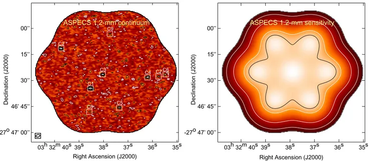
In this process, we produced “clean” maps masking with tight boxes all the continuum sources previously detected in the “dirty” maps with significances above s5 , and cleaning down to a2.5sthreshold. Given the large bandwidth covered by our Figure 1. Left: ALMA 1.2 mm S/N continuum mosaic map obtained in the HUDF. Black and white contours show positive and negative emission, respectively. Contours are shown at2 , 3 , 4 , 5 , 8 , 12 , 20 , ands s s s s s s 40 , with ss = 12.7 Jy beamm −1at thefield center. The boxes show the position of the sources detected with our extraction procedure atS N>3.5. The synthesized beam( ´ 1 2) is shown in the lower left. Right: ALMA 1.2 mm observation PB pattern to represent the sensitivity obtained across the covered HUDF region. PB levels are shown by the black/white contours at levels 0.3, 0.5, 0.7, and 0.9 of the maximum. Both the S/N and PB maps are shown down to PB=0.2.
observations, the contamination by line emission in the continuum map becomes negligible.
Thefinal maps are shown in Figures1and2. The sensitivity in each map declines with respect to the distance from the phase pointing center and, given the smaller PB, declines particularly sharply for the 1.2 mm observations at the outskirts of the mosaicked region. We reach an rms sensitivity of12.7 and 3.8 Jy in the centers of the 1.2 and 3 mm maps,m respectively. The final map average frequencies over the frequency ranges covered are 242 and 95 GHz, respectively.
Finally, we note that while source confusion for individual detections is negligible in these deep ALMA maps, it is at the level where it becomes important for stacking analyses. With an ALMA beam size at 1.2 mm of 1. 7 ´ 0. 9, there are
´
8.47 106beams per deg2. At the bottom flux bin of our number count measurements (see Section 4), we find
´
1.32 105 sources per deg2. This translates into one source per∼64 beams and implies that confusion is not an issue. The same logic applies for the stacking analysis presented below (see Section6). The deepest stacks considered reach a s3 level of 8 μJy at 1.2 mm. Extrapolating the number counts to this flux level, we find about 6.0´105 sources per deg5. This results in one source per 14 beams. According to Helou & Beichman (1990), bright source confusion becomes important
at one source per 22 beams, suggesting that stacking experiments in these ALMA deep maps will be affected. However, this confusion limit depends on the slope of the number counts, and since this slope appears toflatten at these faint flux levels, it is possible that confusion would have a lesser impact at these depths, and in particular on stacking analyses.
2.2. Multiwavelength Data
Our ALMA observations cover a∼1 arcmin2region within the deepest 4.7 arcmin2 of the HUDF: the eXtremely Deep Field (XDF). Available data include Hubble Space Telescope (HST) Advanced Camera for Surveys (ACS) and Wide Field
Camera 3 IR data from the HUDF09, HUDF12, and Cosmic Assembly Near-infrared Deep Extragalactic Legacy Survey (CANDELS) programs, as well as public photometric and spectroscopic catalogs(Coe et al.2006; Xu et al.2007; Rhoads et al.2009; McLure et al.2013; Schenker et al.2013; Bouwens et al.2014; Skelton et al.2014; Momcheva et al.2016; Morris et al. 2015). In this study, we make use of this optical and
infrared coverage of the XDF, including the photometric and spectroscopic redshift information available from Skelton et al. (2014). In addition to the HST coverage, a wealth of optical and
infrared coverage from ground-based telescopes is available in thisfield (see Skelton et al.2014). The HUDF was also covered
by the Spitzer Infrared Array Camera(IRAC) and Multiband Imaging Photometer, as well as by the Herschel Photodetector Array Camera and Spectrometer and the Spectral and Photometric Imaging Receiver(Elbaz et al.2011).
3. RESULTS
3.1. Source Detection and Flux Measurements Source detection was performed using SExtractor(Bertin & Arnouts1996) in the ALMA 1.2 and 3 mm maps prior to PB
correction. We use a minimum area of 5 pixels ( 1. 5) for detection, extracting sources down to 2.5σ, where σ is evaluated locally for each source. Source extraction in the 1.2 mm map was performed beyond the HPBW of our mosaic, out to PB=0.3; however, most sources are detected within PB=0.5, in the central region of the mosaic. Although we extract all sources down to 2.5 , we consider as individuals detections only sources above >3.5s significance. This significance level cut corresponds to roughly 50%–60% fidelity of the sample(see Section3.2). These sources are highlighted
with boxes in Figures1and 2and are listed in Table1. Nine sources are detected in the 1.2 mm map at a significance above 3.5σ. For reference, Table 1 also lists another seven sources with significances between 3.0σ and 3.5σ (our supplementary sample). Given the lower significance Figure 2. Left: ALMA 3 mm S/N continuum mosaic map obtained in the HUDF. Black and white contours show the positive and negative signal, respectively. Contours are shown at2 , 3 , 4 , 5 , 8 , 12 , 20 , ands s s s s s s 40 , with ss = 3.8 Jy beamm −1at thefield center. The boxes show the position of the sources detected in the 1.2 mm map, with our extraction procedure atS N>3.5. The synthesized beam( ´ 2 3 ) is shown in the lower left. Right: ALMA 3 mm observation PB pattern. PB levels are shown by the black/white contours at levels 0.3, 0.5, 0.7, and 0.9. Both the S/N and PB maps are shown down to PB=0.2.
of these sources, we choose not to use them to study the multiwavelength properties of this population. Nevertheless, we can use them to constrain the number counts of faint sources, after correcting for fidelity and completeness. Only one source is detected in the 3 mm map at the >3.5s significance level, corresponding to the brightest detection at 1.2 mm. For this reason, we only show the 1.2 mm detected sources in Figures 1–2.
We computefluxes based on a two-dimensional Gaussian fit centered at the location of the SExtractor detection. In all but one case (discussed below) the sources are unresolved at the resolution and depth of the 1.2 mm observations. We therefore list theflux as the peak flux density value at the source position delivered by the fitting routine. These fitted values are in agreement with the actual pixel values at the position of the sources. We cannot discard the possibility that sources with low significances are indeed being resolved given the relatively small beam size. It is thus unclear what fraction of the flux is being unaccounted for in individual sources.
Only the brightest source in the map is marginally spatially resolved with a measured angular size of (0.520.14) ´ (0.430.26) (PA=49°), and we record the integrated flux in Table1. More details on this source’s properties are given in PaperIV. Since only one source is detected in the 3 mm map, in what follows we concentrate on characterizing the properties of the 1.2 mm sources.
3.2. Fidelity and Completeness
We quantify the occurrence of spurious sources in our 1.2 mm sample by applying the detection routine explained in the previous section to the inverted “negative” map. We thus
compute thefidelity P of our sample as
( ) ( ) ( ) ( ) = -P S N S N S 1 , 1 1.2 mm neg 1.2 mm pos 1.2 mm
where Nneg and Npos are the number of negative and positive
sources, respectively, detected in the map as a function of 1.2 mmflux density.
Figure3shows thefidelity and number of positive detections in our map as a function of 1.2 mm flux density. Not surprisingly, wefind that the fidelity of our sample is a strong function of the 1.2 mmflux density. We reach 100% fidelity at
m
100 Jy(7.8σ) and 50% fidelity at40 Jym (~3.0 ). This meanss that at the 3s level, half of our sources are expected to be spurious, which motivates our choice of a 3.5σ cut for the main sample.
We parameterize thefidelity with 1.2 mm flux density as
( )= ⎧⎨ ( )- + ( ) ⎩ ⎫ ⎬ ⎭ P S S A B 1 2erf log 1.0, 2 1.2 mm 10 1.2 mm
where A=log10(42) and B=1 4, and S1.2 mm is in units of
μJy. We use this parameterization to compute the fidelity level or reliability of our individual detections.
We compute the completeness of our observations by running Monte Carlo simulations on our continuum map. We ingest 10 artificial point-like sources with randomly generated flux levels (between10 and 300 Jy) in the ALMA map. Wem
then run our source detection procedure to identify and compute the fraction of recovered sources (versus the input sources). Recovered artificial sources are matched with the input positions within a radius of 1 , roughly the size of our synthesized beam. Similar to the findings of Fujimoto et al. (2016), the input and recovered flux densities agree well within
Table 1
Sources Detected in the ASPECS 1.2 mm Continuum Map
IAU Name Short Name R.A.1.2 mm Decl.1.2 mm S/N S1.2 mm PB1.2 mm S3 mm PB3 mm OID?
ALMA ASPECS (J2000) (J2000) (μJy) (μJy)
(1) (2) (3) (4) (5) (6) (7) (8) (9) (10)
Main Sample at>3.5 Significances
MMJ033238.54-274634.6a C1 03:32:38.54 −27:46:34.6 39.9 553±14 0.92 31.1±5.0 0.89 Y MMJ033239.73-274611.6a C2 03:32:39.73 −27:46:11.6 10.3 223±22 0.59 <21 0.56 Y MMJ033238.03-274626.5 C3 03:32:38.03 −27:46:26.5 9.6 145±12 0.95 <12 1.00 Y MMJ033236.20-274628.2 C4 03:32:36.20 −27:46:28.2 6.1 87±14 0.89 <17 0.68 Y MMJ033237.35-274645.7 C5 03:32:37.35 −27:46:45.7 5.2 71±14 0.92 <16 0.70 Y MMJ033235.47-274626.6a C6 03:32:35.47 −27:46:26.6 3.9 97±25 0.51 <25 0.45 Y MMJ033235.75-274627.7 C7 03:32:35.75 −27:46:27.7 3.7 70±19 0.67 <21 0.55 Y MMJ033238.57-274648.0 C8 03:32:38.57 −27:46:48.0 3.6 46±13 0.99 <18 0.62 N MMJ033237.74-274603.0 C9 03:32:37.74 −27:46:03.0 3.5 55±16 0.80 <16 0.70 N
Supplemetary Sample at 3.0σ–3.5σ Significance
MMJ033237.36-274613.2 C10 03:32:37.36 −27:46:13.2 3.3 45±14 0.93 <13 0.88 N MMJ033238.77-274650.1 C11 03:32:38.77 −27:46:50.1 3.2 47±14 0.88 <21 0.55 N MMJ033237.42-274650.4 C12 03:32:37.42 −27:46:50.4 3.2 59±18 0.69 <19 0.60 Y MMJ033236.50-274647.4 C13 03:32:36.50 −27:46:47.4 3.2 67±21 0.60 <22 0.52 Y MMJ033236.43-274632.1 C14 03:32:36.43 −27:46:32.1 3.1 46±15 0.85 <16 0.73 Y MMJ033237.49-274649.3 C15 03:32:37.49 −27:46:49.3 3.1 52±17 0.76 <18 0.63 N MMJ033237.75-274609.6 C16 03:32:37.75 −27:46:09.6 3.0 41±14 0.93 <14 0.85 N Notes.Columns: (1), (2) Source full and short names. (3), (4) Position of the 1.2 mm continuum detection in the ALMA 1.2 mm map. (5) Signal-to-noise ratio of the 1.2 mm detection.(6) Flux density at 1.2 mm, corrected for PB. (7) Primary beam correction at the location of the detection in the 1.2 mm mosaic. (8) Flux density at 3.0 mm of the ALMA 1.2 mm continuum detection; upper limits are given at the s3 level.(9) Primary beam correction at the location of the 1.2 mm detection in the 3.0 mm map.(10) Is there an optical counterpart identification for this source (yes or no)?
a
individual source uncertainties. We repeat this process 10 times, for a total of 100 artificial sources. Note that we do not inject all 100 sources in a single step since this would result in significant source blending in the ALMA image.
Figure3 shows the resulting completeness as a function of extracted 1.2 mmflux density. We find that our sample is 100% complete at S1.2 mm~300 Jym (23σ) and 50% complete at
m
~40 Jy (3.0σ). This indicates that at the s3 level, we recover only half of real input sources.
We parameterize the completeness with 1.2 mmflux density as ( )= ( )- ¢ ( ) ¢ + ⎧ ⎨ ⎩ ⎫ ⎬ ⎭ C S S A B 1 2erf log 1.0 3 1.2 mm 10 1.2 mm
where A¢ =log10(35)and B¢ =0.45, and S1.2 mmis in units of
μJy. We use this parameterization to compute the completeness level of our individual detections.
4. NUMBER COUNTS
We use the sources detected in our ALMA HUDF map to compute the number counts at 1.2 mm. We compute the number counts( ( )N Si) in each flux density bin Sias
( )=
å
( ) = N S A P C 1 , 4 i j X j j 1 iwhere A is the effective area of our ALMA mosaic and Xiis the number of sources in each particular bin i. The parameters Pj and Cjcorrespond to thefidelity and completeness at the flux bin i. Since we are limited by the modest number of detections, we compute the cumulative number counts rather than computing differential counts by summing up eachN S( )i over
all measurements >Si. In addition, we extend our number count
measurements down to significances of s3 . While at this level
there is substantial contamination and low detection rate, we can statistically correct the values forfidelity and completeness. As pointed out in the previous section, at the s3 level we reach 50% fidelity and 50% completeness in our sample detection. This implies that these effects cancel out when we compute the number counts. Thus, while we obtain correct number counts at the s3 level, the identification of real sources is correct only in half of the cases.
The uncertainties in the number counts are computed by including the Poissonian errors andflux uncertainties in each individual measurement. The uncertainties in each bin are dominated by the Poissonian errors on Xi; however, at the lowest significance levels the flux uncertainties start to have a significant contribution.
The cumulative number counts ( (N >Sn)) are shown in Figure4. The actual measurements are listed in Table 2. For comparison, we show number count measurements from the literature (Hatsukade et al. 2013; Karim et al. 2013; Ono et al. 2014; Carniani et al. 2015; Oteo et al. 2016; Simpson et al.2015; Fujimoto et al.2016). We scale the flux densities of
the different studies asS1.2 mm=0.4S870,S1.2 mm=0.8S1.1mm,
and S1.2 mm=1.3S1.3 mm (for consistency with Fujimoto
et al.2016).
Our ALMA HUDF observations appear to be in general agreement with these earlier measurements, in particular with the counts obtained by Carniani et al. (2015) and Oteo et al.
(2016). However, our counts are lower by about a factor of 2 in
the flux range S1.2 mm=0.06 0.4– mJy compared to other studies in the literature (Hatsukade et al. 2013; Ono et al.2014; Fujimoto et al.2016). These differences could be
explained by the fact that these studies might be biased as they used pointed observations toward brighter sources in thefield to derive the number counts(i.e., these studies are not unbiased blank-field surveys).
Figure 3. Left: fidelity (top panel) and number of detections (bottom panel) as a function of 1.2 mm flux density of the ASPECS sample (noncumulative). The solid curve is a model for thefidelity. Our sample shows 100% fidelity atS1.2 mm~100 Jym and 50%fidelity at~40 Jy (3.0σ). Right: completeness of our 1.2 mmm continuum sample detection as a function of 1.2 mmflux density. The solid curve shows a model for the completeness behavior as a function of 1.2 mm flux density. Our sample shows 100% completeness atS1.2 mm~300 Jym and 50% completeness at~40 Jy (3.0σ).m
Another possibility is that cosmic variance does play an important role among the different analyses; e.g., the ECDFS, where the HUDF resides, is believed to be underdense of submillimeter sources above∼3 mJy (at 345 GHz) by a factor of ∼2 (Weiß et al.2009). As indicated by several studies, the
ECDFS appears to be underdense in other galaxy populations as well, including BzK galaxies and X-ray and radio sources (e.g., Lehmer et al. 2005; Blanc et al. 2008). However, as
already noted by Weiß et al. (2009), the underdensity appears
to be seen only in the brightest sources, given the steep slope at fainterfluxes (see also Karim et al.2013). Another possibility
is that the differences in number counts between studies come from scatter induced by different analysis techniques and methods. This effect was seen to be dominant compared to statisticalfluctuations in radio surveys (Condon 2007).
5. MULTIWAVELENGTH PROPERTIES OF THE ALMA 1.2 MM SOURCES
5.1. Astrometric Offset
Using the identified millimeter/optical counterpart positions (see below), we measure a systematic astrometric offset of the HST positions of » 0. 3 to the north of the ALMA positions. To check the ALMA registration, we inspected the millimeter calibrators used, finding good astrometric solutions, accurate within 0. 01 with respect to the cataloged radio-based values. Based on the GOODS 2008 data release documentation,30it is clear that a consistent offset( 0. 32) was applied to the GOODS-North astrometric solution but not to the GOODS-South data. Hence, we correct the HST positions by 0 3 to match the ALMA millimeter registration throughout. This is consistent with results from a shallower ALMA millimeter continuum Figure 4. Number counts of ALMA 1.2 mm continuum sources in the HUDF compared with values from the literature. Our data have been corrected to account for completeness andfidelity in the source identification, as discussed in the text. Uncertainties in the number count measurements correspond to Poisson errors. Our measurements span almost two orders of magnitude influx density. Filled circles represent literature measurements obtained at 1.2 mm. Open circles represent measurements from different wavelengths than 1.2 mm and converted to this wavelength. Most of the measurements from the literature at the faint levels are not blank field and are thus biased, since their observations target bright sources in the field (they measure counts around other sources). The Fujimoto et al. (2016) data pointing toward lowerflux densities are based on lensed galaxy clusters.
Table 2
ALMA HUDF 1.2 mm Number Counts
log(Sν) dN dlog( )Sn N(>Sn) dN- dN+
(mJy) (mJy−1) (deg−2) (deg−2) (deg−2)
(1) (2) (3) (4) (5) −1.49 23 132000 3700 43000 −1.24 10 71500 16600 21500 −0.99 3 23700 9400 14700 −0.74 1 9200 5800 11900 −0.24 1 4500 3800 10400
Note.Columns: (1) Flux density bin center (in units of mJy). (2) Number of entries per bin(before fidelity and completeness correction). (3) Number of sources per square degrees.(4), (5) Lower and upper uncertainties (error bars) onN(>Sn).
30
survey of the full HUDF (Dunlop et al. 2016; Rujopakarn et al.2016).
5.2. Identification and SED Fitting
Figure 5 shows the location of the 1.2 mm continuum sources with respect to the optical galaxies in the field. Our blank-field observations encompass a significant number of optical galaxies; however, this is in contrast with the small number of galaxies detected in the millimeter regime. Our sources do not appear to be clustered.
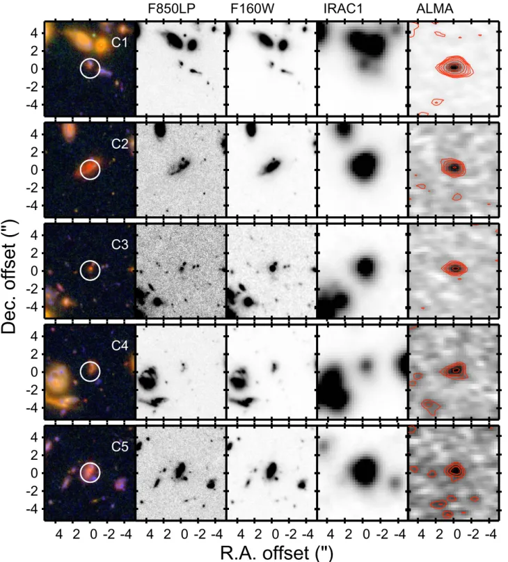
For each individual 1.2 mm continuum detection, we identify optical counterparts within a radius of 1 from the millimeter position. We choose this search radius since it is well matched to the ALMA 1.2 mm synthesized beam( ´ 1. 7 0. 9). Figure6
presents multiwavelength cutouts for individual detections. Seven of the continuum sources with significances>3.5 haves an obvious counterpart in the HST images, and five of these have an available spectroscopic redshift(see Table3; Skelton et al. 2014). The other two millimeter detections, with lower
significances in our sample (∼3.5σ–3.6σ), do not show an obvious counterpart. Four out of seven sources with signi fi-cances between 3.0σ and 3.5σ do not have an optical counter-part (Table 1), consistent with the fidelity level at this
significance, and indicating that some or all of these are likely spurious millimeter detections. Another possibility would be that these are faint dusty galaxies at higher redshifts (as in HDF850.1; see Walter et al.2012).
We fit the SED of the continuum-detected galaxies using the high-redshift extension of MAGPHYS (da Cunha et al. 2008, 2015). We use the available 26 broad- and
medium-bandfilters in the optical and infrared regimes, from the U band to Spitzer IRAC 8μm. We here also include the ALMA 1.2 mm dataflux densities; however we note that the
optical/infrared data have a much stronger weight given the tighter constraints in this part of the spectra. We do not include Herschel photometry in the fits since its angular resolution is very poor, being almost the size of our target field for some of the IR bands. The Herschel photometry is thus heavily blended.
For each individual galaxy, we perform SED fits to the photometry fixed at the best available redshift. MAGPHYS delivers estimates for the stellar masses, star formation rate (SFR), dust mass, and IR luminosity. Even though for most galaxies we do not have photometric constraints on the observed IR SED,MAGPHYS employs a physically motivated prescription to balance the energy output at different wavelengths. Thus, estimates on the IR luminosity and/or dust mass come from constraints on the dust-reprocessed UV light, which is well sampled by the UV-to-infrared photometry. For some galaxies with faint optical/near-infrared fluxes or with weak constraints in the photometry,MAGPHYS is able to output only some of the parameters with enough accuracy (e.g., stellar masses). How-ever, all the optical counterparts of our millimeter-detected sample are sufficiently bright to yield good parameters derived by MAGPHYS. The properties derived for individual sources detected in our ALMA 1.2 mm continuum are shown in Table3. Figure7shows the distribution of stellar masses and SFRs of our ALMA 1.2 mm continuum sources. For comparison, we show the stellar masses and SFRs derived in the same way for field galaxies located within the field of view of our ALMA map(within PB=0.4) and selected to be in a redshift range that matches the redshifts of our ALMA continuum sources. We limit the comparison sample to sources with mF850LP and
<
mF160W 27.5mag AB, in order to ensure good SEDfits and
derived properties. Wefind that the faint DSFG population, as revealed by our ALMA 1.2 mm sources, has higher stellar masses and SFRs than the field galaxy population at similar Figure 5. HUDF multicolor image (F435W, F850LP, F105W) of the region covered by our 1 mm ALMA observations. The boxes show the position of the 1.2 mm sources detected with our extraction procedure atS N>3.5. The white contour shows the coverage of our ALMA observations down to PB=0.2.
redshifts, yet much lower values than those found in brighter DSFGs (i.e., SMGs). Our sources show a median stellar mass of 4.0´1010 M and a median SFR of 40M☉ yr−1,
which are significantly lower than the typical values for SMGs, with stellar masses in the range (0.8 3.0– )´1011M☉ (e.g.,
Michałowski et al. 2010; Hainline et al. 2011; Michałowski et al. 2012; Simpson et al. 2014; da Cunha et al. 2015; Koprowski et al. 2016) and SFRs well above100M☉ yr−1
(e. g., Casey et al. 2014).
5.3. Redshift Distribution
Since most of the galaxies detected at>3.5 in our samples have available spectroscopic redshifts from the various surveys of the HUDF, we investigate the redshift distribution of our sample.
Figure 8 shows the redshift distribution for our ALMA continuum sources that have an optical counterpart compared with various millimeter-selected samples of bright DSFGs from the literature.
Figure 6. Multiwavelength image thumbnails toward the ALMA 1.2 mm continuum detections (>3.5 ). From left to right, we show an optical–near-infrared false-s
We find that all the 1.2 mm continuum sources detected above 3.5s in our sample are located in the redshift range
– =
z 1 3, and none are associated convincingly with a galaxy at >
z 3. This excludes the source candidates without counter-parts. While this may only reflect the low number statistics due to the small area of the sky covered, it also supports the idea that the population of galaxies discovered in our deep ALMA 1.2 mm continuum map significantly differs from the popula-tion of DSFGs found in shallower but wider (sub)millimeter surveys. The DSFG samples from the literature are found to have median redshifts ranging fromz~2.1 toz~3.1, with a possible tail extending out to z~6 (Chapman et al. 2005; Smolcic et al.2012; Yun et al.2012; Riechers et al.2013; Weiß et al.2013; Simpson et al.2014; Miettinen et al.2015; Dunlop et al.2016; Strandet et al.2016). We find that our faint ALMA
millimeter-selected galaxies, however, have a median redshift
=
z 1.7 0.4. The uncertainty here corresponds to the scatter in the redshifts. This median redshift is significantly lower than the typical redshift of bright DSFGs, irrespective of the nature the DSFG samples (lensed or unlensed) or the selection wavelength (870 μm or 1.2 mm). Statistically, this would not
be significantly affected if the two sources without counterparts were located at z>2 given the small scatter in the redshift distribution.
While the SMG and fainter millimeter source populations are obviously different as reflected by the significantly lower 1.2 mmfluxes, this is the first time that we are able to evaluate the redshift distribution of the faintest 1.2 mm emitters in a contiguous blankfield (belowS1.2 mm=0.5mJy). Other studies reaching down to the faint millimeter flux regime are mostly based on archival data of different individualfields where the faint millimeter emitters are not the main targets(e.g., Carniani et al. 2015; Oteo et al. 2016; Fujimoto et al.2016) or do not
have the excellent deep multiwavelength coverage of the HUDF in order to address this issue.
The decline in the median redshift with decreasing flux density for millimeter-selected sources was recently predicted by phenomenological models of galaxy evolution(Béthermin et al. 2015). Even though the prediction does not assess the
redshifts for populations with 1.2 mm flux densities below 0.2 mJy, already at thisflux level they find a median redshift of ∼2 compared to the much higher ~z 3 predicted for brighter Figure 6. (Continued.)
SMGs selected at 1.2 mm. By extrapolating their prediction down to aflux density cut of~35 Jy (our 3σ cut), we find anm expected median redshift of ∼1.5. This value is in good agreement with our measurements and supports the fact that the redshift distribution of millimeter-selected galaxies is affected by theflux density cut.
5.4. Starburst versus Main Sequence
An important result from multiwavelength surveys in the past decade has been the determination that typical star-forming galaxies form a tight linear relationship in the SFR–Mstarsplane
out to z~3(e.g., Brinchmann et al.2004; Daddi et al.2007; Elbaz et al. 2007; Noeske et al. 2007; Pannella et al. 2009; Karim et al. 2011; Rodighiero et al. 2011; Whitaker et al.
2012). Sources that lie close to this star formation relationship
have been termed main-sequence galaxies. Galaxies lying above this sequence are called starbursts, as they have excess star formation activity with respect to most galaxies in the main sequence for the same stellar mass, or higher specific star formation rates (sSFRs). This sequence has been observed to evolve with redshift, with higher SFRs for a given stellar mass at increasing redshifts (Whitaker et al. 2012), and it has also
been claimed toflatten at the high stellar mass end (Whitaker et al.2012,2014; Lee et al.2015; Pannella et al.2015).
Figure9 shows the stellar mass versus SFR derived using MAGPHYS for all HST-detected galaxies at < <1 z 3 con-tained within our ALMA HUDF survey area(within PB =0.4 of our 1.2 mm map) and restricted to be brighter than 27.5 AB mag in the F850LP and F160W bands. We show the sources detected in our 1.2 mm observations(>3.5 ) and compare withs the main-sequence fit derived by Whitaker et al. (2014). We
find that all the millimeter-detected galaxies at z<2 are located within the scatter of the main sequence atz~1 2 and– taking into account the uncertainties in the derived properties. Similarly, the only millimeter detection atz>2(ASPECS C1) is also well within the scatter of the main sequence at Table 3
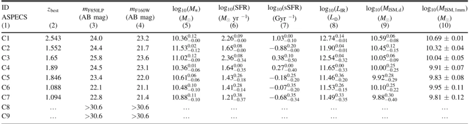
Derived Properties for the ALMA HUDF 1.2 mm Sources
ID zbest mF850LP mF160W log (10M*) log10(SFR) log10(sSFR) log (10LIR) log (10MISM,d) log (10MISM,1mm)
ASPECS (AB mag) (AB mag) (M) (M yr -1) (Gyr )-1 (L☉) (M) (M)
(1) (2) (3) (4) (5) (6) (7) (8) (9) (10) C1 2.543 24.0 23.2 10.36-0.120.00 2.26-0.090.00 1.03-0.000.10 12.74-0.140.01 10.59-0.060.08 10.69±0.01 C2 1.552 24.4 21.7 11.53-0.020.12 1.65-0.080.00 -0.88-0.200.00 11.90-0.040.01 10.45-0.120.15 10.32±0.04 C3 1.65 25.8 23.6 11.02-0.120.09 2.36-0.080.34 0.38-0.100.50 12.54-0.040.32 10.05-0.060.09 10.04±0.05 C4 1.89 24.5 23.1 10.36-0.010.06 1.64-0.000.35 0.27-0.000.40 11.65-0.000.33 10.00-0.250.25 9.91±0.07 C5 1.846 23.4 22.0 10.61-0.060.06 1.43-0.260.18 -0.18-0.250.20 11.46-0.360.20 9.92-0.280.29 9.83±0.08 C6 1.088 22.1 21.1 10.48-0.100.10 1.41-0.280.14 -0.07-0.350.20 11.53-0.260.15 10.10-0.250.22 9.95±0.11 C7 1.094 22.8 21.4 10.88-0.110.10 1.21-0.380.37 -0.68-0.350.34 11.49-0.330.35 9.88-0.300.40 9.81±0.12 C8 K >30.6 >30.6 K K K K K K C9 K >30.6 >30.6 K K K K K K
Note.Columns: (1) Source name. (2) Best available redshift estimate. If spectroscopic, we quote three decimal places. If photometric, we quote only two decimal digits. References: CO-based redshifts, confirmed with optical spectroscopy for C1, C2, and C6 (PaperI; PaperIV; Skelton et al.2014). Optical redshifts for C3, C4, C5, and C7(Skelton et al.2014). Photometric redshifts for C3 and C4 from Coe et al. (2006) and Skelton et al. (2014). (3), (4) AB magnitudes in the F850LP and F160W HST Bands. Uncertainties in quoted values range between 0.01 and 0.05 mag.(5) Stellar mass derived through SED fitting. (6) SFR derived through SED fitting. (7) Specific SFR (SFR/M*). (8) IR luminosity output from MAGPHYS. (9) ISM mass derived from the dust mass delivered by MAGPHYS and a gas-to-dust ratio
dGDR= 200.(10) ISM mass obtained from the 1.2 mm flux and the calibrations from Scoville et al. (2014).
Figure 7. Distribution of stellar masses and SFRs (obtained from SED fitting) for the galaxies detected in our ALMA 1.2 mm continuum map. For comparison, the distribution offield galaxies in the relevant redshift range is shown.
Figure 8. Redshift distribution for (sub)millimeter-selected galaxies. The y-axis shows the number of galaxies in each bin, normalized to the total number of galaxies in each sample. The black solid line shows the redshift distribution of our ALMA HUDF 1.2 mm detections( s>3 ). The gray and green solid lines show the redshift distribution for the 1.2/1.4 mm selected samples of SMGs in the COSMOS (Miettinen et al.2015) and SPT surveys (Weiß et al.2013), respectively. The dashed orange and blue lines show the 850/870 μm selected SMGs from Chapman et al.(2005) and from the ECDFS (Simpson et al.2014).
– =
z 2.0 2.5. We thus conclude that our faint ALMA 1.2 mm continuum sources are main-sequence galaxies at z~1 3.–
Recently, Hatsukade et al. (2015) studied the properties of
four 1.3 mm detected sources withfluxesS1.3 mm>0.2mJy(at least two times brighter than our sources). They find that these four galaxies are in the main sequence, with redshifts
– =
z 1.3 1.6. However, those sources were selected in fields where these faint millimeter emitters were not the primary target. Most of these continuum sources lie in a dense environment atz~1.3, and it is thus unclear how representa-tive their redshift and properties are of thefield population.
All the sources shown in Figure 9 lie within the uniform sensitivity region of our 1.2 mm mosaic, within PB =0.4. However, there are a few of them that were not detected in the 1.2 mm continuum even though they have similar SFRs and stellar masses to the detected sources. This could partly be attributed to uncertainties in the SEDfitting procedure or to the fact that some galaxies would be located at the very edges of our mosaic. However, it is possible that the nondetection of these sources could also be due to differences in the individual physical properties of these sources. For instance, galaxies with lower dust temperatures or masses would tend to have lower fluxes at 1.2 mm, or they could just be dust poor. In Section 6
we address this issue using stacking analysis.
6. STACKING ANALYSIS
We use the stacking analysis to investigate the nature of the fainter galaxy population not detected at the achieved sensitivity limit of our ALMA 1.2 mm mosaic. To perform the stacking, we extract smaller images, ´ 9 9 in size, from the final clean ALMA 1.2 mm continuum mosaic, centered at the position of sources that were selected from an independent galaxy catalog (see below). Subimages of the same size are simultaneously extracted from the PB sensitivity mosaic map. All these subimages are then combined together, to construct a weighted average using the PB sensitivity map as the weight. The noise in this average image is then obtained from an
annulus around the central position with an initial and final radius of 4 and 12 pixels, respectively (1 pixel=0 3). A summary of the stacking analysis results is shown in Figure10
and listed in Table4.
6.1. Nature of Undetected Galaxies
Using stacking, we first investigate the emission from galaxies individually undetected at the3.5 level in the ALMAs 1.2 mm continuum map as a function of redshift. If these galaxies were to follow a similar redshift distribution to that of the detected galaxies, then we would expect on average that the galaxies in the 1< <z 2 range would have more 1.2 mm continuum emission than those in other redshift ranges. Figure 10 shows the stacked emission of galaxies in three different redshift ranges(samples z1, z2, and z3; see Table4).
All samples have been selected to have M* >109M☉ and
<
z 4, and sources that enter the stack were required to lie 3. 5 away from the location of thefive most significant individual continuum detections to avoid contamination. The restriction to have a relatively high stellar mass is specifically to not down-weight the stack signal. To avoid including passive evolving galaxies with no star formation activity in the stacks, we only select galaxies that are located within and above the main sequence (see Figure 9), taking into account a conservative
0.5 dex of scatter in the sequence relationship. The main-sequence trends as a function of redshift are taken from Whitaker et al.(2014). Additionally, to limit our sample only to
galaxies with good measured SED fits, we require that the sample galaxies have magnitudes brighter than 27.5 AB in the F850LP and F160W bands. Galaxies detected at the>3.5s level in the 1.2 mm continuum have been excluded from the stacked samples. Using this selection, we only detect 1.2 mm emission from galaxies at1 < <z 2(the z2 sample). In all the other redshift samples, we do notfind significant emission and thus place s3 limits on the 1.2 mmflux densities (see Table4).
This implies that most of the underlying millimeter emission that is not directly detected in our ALMA continuum map Figure 9. Stellar mass vs. SFR for the galaxies covered in our ALMA HUDF 1.2 mm map in the two relevant redshift bins. The large yellow circles show the ALMA 1.2 mm continuum sources(>3.5 ). The small blue circles show field galaxies in either thes 1.0< <z 2.0 or2.0< <z 3.0 redshift bin. Field galaxies are restricted to be brighter than 27.5 AB mag in the F850LP and F160W bands. For comparison, the orange and magenta curves represent the best second-order polynomialfits of the star formation sequence at1.0< <z 1.5,1.5< <z 2.0, and2.0< <z 2.5 for the left and right panels, respectively(Whitaker et al.2014).
comes from galaxies located at similar redshifts to those of the individually detected galaxies, which have matching redshift distribution with a median z=1.65.
To shed light on whether the most massive or star-forming galaxies could have underlying 1.2 mm emission, we stack on different galaxy samples split in stellar mass and SFR. We use three samples divided by stellar mass and three samples divided
by SFR(see Table4). We apply the same restrictions as for the
redshift samples, including the limit in stellar mass, the requirement that the galaxies lie within and above the main sequence, and the magnitude limit in the optical/near-infrared bands. The galaxies used in these stacks are represented by blue symbols in Figure 9 (this figure does not show galaxies at
<
z 1 andz>3).
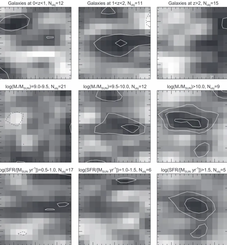
Figure 10. Stacked 1.2 mm continuum on the location of galaxies selected as summarized in Table4(see also text): galaxies selected in the redshift, stellar mass, and SFR ranges are shown in the top, middle, and bottom panels, respectively. Sources individually detected in the 1.2 mm map at S/N > 3.5 are not included in the stacks. The images shown are 3. 6´ 3. 6 in size. Solid white and dashed black contours represent the positive and negative signal, respectively. Contours start at2s in steps of1 .s
Figure10 (middle and bottom panels) shows the results of
this exercise. From the three stellar mass samples, only the samples m2 and m3 present a tentative detection of the stacked 1.2 mm emission. For sample m1, we place a s3 upper limit. This indicates that less massive galaxies have fainter millimeter continuum emission. Note that the stacked detection for the m2 sample is offset from the center, the reason for this shift being unclear since we are excluding sources near the most significant 1.2 mm sources. It is possible that this shift is related to the low S/N of the signal.
By stacking in samples that were selected based on their UV-derived SFRs (derived from SED fitting), we find a clear detection for the s3 sample, which includes all galaxies with SFRUV>30Myr−1. This is consistent with the detection of
emission in the mass-selected samples m2 and m3, which have concordantly high median UV-derived SFRs. Note that most of the galaxies individually detected at 1.2 mm comply with the s3 sample selection. Thus, the detection of stacked continuum signal in the s3 sample implies that the individually undetected galaxies are just below the detection threshold of our survey, showing on average lower millimeter emission than the individually detected galaxies. The reason for this could be due to uncertainties in the derived stellar masses and SFRs, as well as different physical properties such as lower dust content (lower dust masses).
In summary, wefind that most of the millimeter continuum emission of undetected galaxies is produced by galaxies in the redshift rangez=1 2– (sample z2). When we make stacks on stellar mass, we obtain detections for the stellar mass ranges
☉
- M
109.5 10.0 and
☉
>1010M (samples m2 and m3). These
stellar mass bins have median UV-derived SFRs in the range of
– ☉
~3 30M yr−1. When we explicitly consider galaxy samples with UV-derived SFRs, we only obtain a detection for galaxies with SFRs>30M☉yr−1(but not for the –10 30M☉yr−1bin).
These stacked detections reach down to 1.2 mm continuum fluxes of ∼10 μJy.
6.2. Stacking in the 3 mm Continuum
Since there is only one significant source in the 3 mm continuum map, we use the stacking analysis to measure the average 3 mm emission from all the sources that were detected at>3.5 in the 1.2 mm map. The result of this procedure iss shown in Figure 11. Including all the 1.2 mm sources in the stack, we find an average flux density of S3 mm,all=
m
12 3 Jy. Masking the individually detected source in the 3 mm map, we find an average flux density of
m
=
S3 mm,masked 9 3 Jy. Using the same stacking procedure
and adopting the same samples on the 1.2 mm map (i.e., stacking the 1.2 mm detected sources to obtain the average 1.2 mm flux), we find S1.2 mm,all=195 11mJy and
m
=
S1.2 mm,masked 125 12 Jy, respectively.
The ratio between these measurements can now be used to obtain an estimate of the dust emissivity index β. We use a single-component modified blackbody dust model in the optically thin regime of the formSn µ(1 -e-tn)B Tn( )d (see Table 4
Results from the Stacking Analysis
Samplea Selectionb zmedc log10(SFRUV, med)d log10( *M,med) Nobje S1.2 mmf
(M☉yr−1) (M☉) (μJy) (1) (2) (3) (4) (5) (6) (7) z1 z=0 1– 0.76±0.19 0.84±0.52 9.78±0.49 12 <13 z2 z=1 2– 1.22±0.20 0.52±0.63 9.45±0.43 11 12±4 z3 z=2 4– 2.45±0.41 0.75±0.36 9.48±0.31 15 <13 m1 log10(M* M☉)=9.0 9.5– 1.63±0.80 0.46±0.35 9.25±0.14 21 <8 m2 log (10M* M☉)=9.5 10.0– 1.29±0.95 0.93±0.35 9.78±0.12 12 113.0 m3 log10(M* M☉)>10.0 1.10±0.79 1.00±0.51 10.2±0.22 9 19±5 s1 log10(SFR) =0.5-1.0 M☉yr−1 1.67±0.93 0.70±0.16 9.58±0.36 17 <12 s2 log10(SFR) =1.0-1.5 M☉yr−1 2.45±0.78 1.02±0.13 9.81±0.27 6 <15 s3 log10(SFR) >1.5 M☉yr−1 1.05±0.48 1.73±0.21 10.2±0.36 5 25±8
Note.Columns: (1) Sample name. (2) Selection imposed for this sample. In all cases, we excluded the individually detected sources with>3.5 . We limited thes
samples to have M* >109M☉, to be located within PB=0.4, and to lie 3. 5 away from the five most significant 1.2 mm continuum detections to avoid
contamination. Additionally, in order to reject non-star-forming sources in our stacks(i.e., old passive evolving galaxies), we restricted the samples to reside above the main sequence including its intrinsic scatter at the relevant redshift range(i.e., sources above MS-0.5 dex), using the calibrations from Whitaker et al. (2014). Only sources with mF850LPandm160W<27.5mag AB were included, in order to retain sources with good SEDfits. (3) Median redshift of the selected sample. (4) Median
SFR obtained from the optical/near-infrared photometry with MAGPHYS. (5) Median stellar mass obtained from the optical/near-infrared photometry with MAGPHYS. (6) Number of objects that entered the stack. (7) Average flux density at 1.2 mm obtained from the stacking procedure.
Figure 11. Stacked 3 mm emission at the location of the 1.2 mm detected sources ( ´15 15 in size). The left panel shows the stacked map when including all sources. The right panel shows the stacked map when including all but the brightest 1.2 mm source, which was also individually detected at 3 mm. White and black contours represent positive and negative emission, respectively. The contours are shown in steps of1 starting ats 2 .s The Astrophysical Journal,833:68(20pp), 2016 December 10 Aravena et al.
Weiss et al. 2007), whereS is the observedn flux density,B isn
the Planck function, and Td is the dust temperature. It can be
shown that in the Rayleigh–Jeans (RJ) limit, ( ( ) ( )) ( ) ( ) b n n n n = log S S -log 2, 5 1 2 1 2
where S( )n1 and S(n2) are the flux densities measured at
frequencies n1and n2, respectively. Note that at the observed
frequencies it is valid to assume the optically thin and RJ approximations.
For the galaxy individually detected in the 1.2 and 3 mm maps (ASPECS C1), we find b =1.30.2. For the stack sample that includes all the sources, we find b =1.10.3. Similarly, for the masked sample wefind b =0.90.4. This result suggests a significantly lower dust emissivity index for the faint population of DSFGs than what has been typically found in galaxies in the local universe and the Milky Way, and also at high redshift, with β ranging from 1.5 to 2.0 (e.g., Chapin et al. 2009; Draine 2011; Dunne et al. 2011; Planck Collaboration et al.2011). Note that given the relatively small
beam size of the 1.2 mm observations, we could be missing flux that could contribute to a larger β value. Similarly, the stacked signal detected at 3 mm is weak, and its detection is thus marginal. Both issues could thus be affecting this result. Another possible cause for this lowβ value is the fact that we are tracing fluxes at wavelengths that could receive contrib-ution from free–free emission. This would tend to increase the flux at 3 mm, resulting in larger β. Finally, it is worth mentioning that due to the higher cosmic microwave back-ground temperature with redshift, we would expect to see an increase in the averageβ value with increasing redshift. Larger samples of faint DSFGs are needed to provide better constraints on this subject.
7. ISM PROPERTIES
7.1. Gas Masses from Dust, and Caveats
A useful method to compute ISM masses in galaxies has been the use of the dust mass as a proxy for the ISM content (Leroy et al. 2011; Magdis et al. 2011; Magnelli et al. 2012; Scoville et al. 2014; Genzel et al. 2015). Recently, Scoville
et al. (2014) argued that under reasonable assumptions about
the dust properties, reliable ISM mass measurements can be made based on flux measurements made in the RJ tail of the dust. The method was calibrated using massive galaxies at low and high redshift and assuming afixed gas-to-dust ratio, which is expected to be fairly constant for a relatively ample range in properties(see Scoville et al.2014, for details), and assumes a fixed dust temperature ofTd =25K. Note that there is a weak dependance of this method on Td, since we are probing the RJ
part of the spectrum. Following Scoville et al. (2014), we
compute the ISM mass in units of1010M☉as
( ) n ( ) = + G G n - ⎜⎛ ⎟ -⎝ ⎞⎠ M 1.2 1 z S D 350 , 6 ISM 4.8 obs 3.8 0 RJ L 2
where DLis the luminosity distance in Gpc at redshift z, and Sν is the measuredflux density in mJy at the observing frequency
nobs(in GHz). GRJis a correction factor that takes into account
the deviation from the RJ limit as we approach higher redshifts. This factor depends on z, Td, and nobsand becomes G =0 0.76at
z=0 for n = 242obs GHz and Td=25 K. This method to
compute ISM masses assumes a dust emissivity index b = 1.8, which we use throughout for consistency with other studies.
MAGPHYS also delivers an estimate of the dust mass (Md)
using the median of the dust mass posterior probability when fitting the available photometry. From this dust mass estimate, and under the assumption of a fixed gas-to-dust ratio (dGDR) and that the ISM is mostly molecular, one can obtain a measurement of the gas mass as Mgas=dGDRMd. For local
galaxies it has been found that typically dGDR~ 72(Sandstrom
et al. 2013); however, metallicity-dependent variations are
likely to play a significant role (e.g., Rémy-Ruyer et al.2014).
For the typical stellar masses of our sources(~1010 11- M) and
assuming that local calibrations apply, we would expect metallicities close to the solar value, 12 + log(O/H) ∼ 9 (Tremonti et al. 2004). However, since the metallicities are
lower at high redshift, the typical stellar masses of our sample imply metallicities of∼8.4 at ~z 1.5(Yabe et al.2014; Zahid et al. 2014). This metallicity value would translate into
dGDR~ 200 (Rémy-Ruyer et al. 2014). Hence, we adopt this value to convert the dust masses obtained withMAGPHYS into gas mass estimates.
PaperIV provides a detailed discussion of the different available methods to compute the gas masses, based on the CO measurements for four sources in the ASPECS field. From Table3, wefind that the gas masses obtained using MAGPHYS SED fitting are consistent with the ISM estimates from the Scoville et al. method for the assumed dGDR. PaperIVfinds that
the gas estimates following Scoville et al. and theMAGPHYS SEDfitting methods underpredict the gas masses by a factor of
–
~3 4 compared to the CO-based estimates. There are several reasons that could explain this discrepancy, including (i) a combination of high excitation and low aCO values in the CO
measurements, (ii) systematics in the calibration of the dust-based measurements, and(iii) different spatial distributions of dust and molecular gas within individual galaxies(see PaperIV
for details). Another important issue is that the Scoville et al. (2014) calibration uses a fixed dGDR value assuming solar
metallicity. This assumption is reasonable for massive galaxies (~1011M☉) as applied in their study; however, it may
potentially underestimate the gas masses for less massive, lower-metallicity galaxies, for which a higher dGDR should
be used.
Most importantly, perhaps, is the fact that the Scoville et al. (2014) calibration uses a gas-to-dust ratio fixed value for a solar
metallicity. This assumption is reasonable for massive galaxies as applied in their study (~1011M☉); however, it will likely
result in lower gas masses for less massive, lower-metallicity galaxies, for which a higher dGDR should be used.
Despite these uncertainties, the dust-based estimates con-stitute the only means to provide a measurement of the gas masses in our 1.2 mm continuum-detected sources, given that most of them do not have CO line detections. Table3lists the gas masses obtained using both the Scoville et al. and the MAGPHYS SED fitting methods. In what follows we only use the ISM masses obtained with the Scoville et al. method as a measure of the total molecular gas mass, under the assumption that most of the ISM of high-redshift galaxies is in the form of molecular gas.
7.2. Gas Depletion Timescales and Fractions
Figure 12 shows the ISM mass (using the Scoville et al. method) versus SFR (derived using SED fitting) for the