2020-06-17T13:09:19Z
Acceptance in OA@INAF
Are fractured cliffs the source of cometary dust jets? Insights from OSIRIS/Rosetta
at 67P/Churyumov-Gerasimenko
Title
Vincent, J. -B.; Oklay, N.; PAJOLA, MAURIZIO; Höfner, S.; Sierks, H.; et al.
Authors
10.1051/0004-6361/201527159
DOI
http://hdl.handle.net/20.500.12386/26108
Handle
ASTRONOMY & ASTROPHYSICS
Journal
587
Number
DOI:10.1051/0004-6361/201527159
c ESO 2016
Astrophysics
&
Are fractured cliffs the source of cometary dust jets?
Insights from OSIRIS/Rosetta at 67P/Churyumov-Gerasimenko
J.-B. Vincent
1, N. Oklay
1, M. Pajola
2, S. Höfner
1,3, H. Sierks
1, X. Hu
1,3, C. Barbieri
4, P. L. Lamy
5, R. Rodrigo
6,7,
D. Koschny
8, H. Rickman
9,10, H. U. Keller
3, M. F. A’Hearn
11,12,1, M. A. Barucci
13, J.-L. Bertaux
14, I. Bertini
2,
S. Besse
8, D. Bodewits
11, G. Cremonese
15, V. Da Deppo
16, B. Davidsson
9, S. Debei
17, M. De Cecco
18,
M. R. El-Maarry
19, S. Fornasier
13, M. Fulle
20, O. Groussin
5, P. J. Gutiérrez
21, P. Gutiérrez-Marquez
1, C. Güttler
1,
M. Hofmann
1, S. F. Hviid
22, W.-H. Ip
23, L. Jorda
5, J. Knollenberg
22, G. Kovacs
1,24, J.-R. Kramm
1, E. Kührt
22,
M. Küppers
25, L. M. Lara
21, M. Lazzarin
4, Z.-Y. Lin
23, J. J. Lopez Moreno
21, S. Lowry
26, F. Marzari
4, M. Massironi
2,
F. Moreno
21, S. Mottola
22, G. Naletto
27,2,16, F. Preusker
22, F. Scholten
22, X. Shi
1, N. Thomas
19,
I. Toth
28,5, and C. Tubiana
1(Affiliations can be found after the references) Received 10 August 2015 / Accepted 4 December 2015
ABSTRACT
Context.Dust jets (i.e., fuzzy collimated streams of cometary material arising from the nucleus) have been observed in situ on all comets since the Giotto mission flew by comet 1P/Halley in 1986, and yet their formation mechanism remains unknown. Several solutions have been proposed involving either specific properties of the active areas or the local topography to create and focus the gas and dust flows. While the nucleus morphology seems to be responsible for the larger features, high resolution imagery has shown that broad streams are composed of many smaller jets (a few meters wide) that connect directly to the nucleus surface.
Aims.We monitored these jets at high resolution and over several months to understand what the physical processes are that drive their formation and how this a↵ects the surface.
Methods.Using many images of the same areas with di↵erent viewing angles, we performed a 3-dimensional reconstruction of collimated jets and linked them precisely to their sources on the nucleus.
Results.We show here observational evidence that the northern hemisphere jets of comet 67P/Churyumov-Gerasimenko arise from areas with sharp topographic changes and describe the physical processes involved. We propose a model in which active cli↵s are the main source of jet-like features and therefore of the regions eroding the fastest on comets. We suggest that this is a common mechanism taking place on all comets.
Key words.comets: general – comets: individual: 67P/Churyumov-Gerasimenko 1. Introduction
In March 1986, the Giotto mission flew by the nucleus of comet 1P/Halley. One of its many discoveries was the realization that cometary activity is not evenly distributed across the illuminated surface. Indeed, it appeared that most of the nucleus was dark and seemingly inactive, while a few percent of the surface gave rise to strong collimated flows of gas and dust, commonly re-ferred to as “jets”. In the following 30 yr, five di↵erent cometary nuclei have been visited by space probes, one of them twice (9P/Tempel 1). Fly-by missions provided tremendous data, but by definition could only observe their target at a fixed heliocen-tric distance and for a short time. This led to a better description of cometary jets, but no definite answer as to what the physical processes driving them are and what they mean for the nucleus surface evolution. Several solutions have been proposed: some involve localized physical mechanisms on the surface and in the subsurface (see review inBelton 2010) and explain jets as a re-sult of these surface inhomogeneities. Alternative models con-sider instead purely dynamical processes involving the focusing of gas flows by the local topography (Keller et al. 1994;Crifo et al. 2002), without the need for specific surface properties. The real mechanism seems more likely to be a combination of both processes. While large scale jets are a↵ected by the topography,
high-resolution data has shown that these features are a collec-tion of much smaller jets, which can be traced back all the way down to the surface, pointing to areas with di↵erent properties than their surroundings.
In his review of mechanisms producing collimated outflows,
Belton(2010) proposes a nomenclature of di↵erent types of jet-like activity. Type I describes dust release dominated by the sub-limation of H2O through the porous mantle; Type II is controlled
by the localized and persistent e↵usion of super-volatiles from the interior; while Type III is characterized by episodic releases of super-volatiles.
Type I jets do not appear to be associated to specific mor-phology and are generally broader and more di↵use than other features. On 67P/Churyumov-Gerasimenko (hereafter 67P), this would be the case for the largest jet arising from Hapi region, the interface between the two lobes of the nucleus, since late July 2014. The source of this feature could not be associated with a particular terrain, other than the whole smooth surface of Hapi itself, which also shows a brighter and bluer average spectrum in the visible and infrared (Sierks et al. 2015;Fornasier et al. 2015;
Lara et al. 2015;Lin et al. 2015;Capaccioni et al. 2015). Type II jets, also called filaments, display a much more collimated struc-ture and have been traced back to specific regions of cometary nuclei. For instance, on 81P/Wild 2, they could be associated
to the walls of large, vertical sided pits (Brownlee et al. 2004;
Sekanina et al. 2004). On 9P/Tempel 1, such jets were also linked to a ragged area bordering a large smooth terrain and, in particular, to the scarped edge of this terrain (Farnham et al. 2007). Type III are more sporadic events, probably related to micro-outbursts or other explosive processes.
To progress on this topic, it is necessary to have a longer time coverage of activity and high resolution data of the nu-cleus showing how the surface changes in active areas. ESA’s Rosetta space probe is observing comet 67P over two years of a nominal mission, and this has allowed us to achieve a detailed characterization of the comet’s diurnal and seasonal evolution.
This paper describes how we have linked jets to active sources observed from arrival in August 2014 (3.6 AU) to equinox in May 2015 (1.6 AU). During that time, the subsolar latitude migrated from +42.4 to –5.7 , therefore the results we present here apply only to the northern summer on 67P. We dis-cuss in Sect.4how this work can be extrapolated to other regions and di↵erent comets.
Although the jets characterized in this paper could be de-scribed as Type II in the above nomenclature, we see that they are not necessarily related to the presence of super volatiles and can very well be driven by water sublimation alone, if there is some morphologic control of the flow. In that sense they would be more like a small scale Type I or a new type altogether. 2. Methods
2.1. Observations
The OSIRIS instrument is composed of two elements: a narrow angle camera (NAC, FoV = 2.18 ) and a wide angle camera (WAC, FoV = 11.89 ), both equipped with sets of filters cho-sen to investigate the composition of nucleus and coma (Keller et al. 2007). We typically monitored gas and dust activity with the WAC, about once every two weeks for heliocentric distances greater than 2 AU, and once per week afterward. The nomi-nal sequence had a set of observations once per hour for a full comet rotation (12 h). As both Rosetta and the comet were com-ing closer to Earth, the data volume available increased, and we updated the observational sequence to one set of observations every 20 min for 14 h. This gives us a good coverage of the diurnal and seasonal evolution of the comet.
Dust jet observations consist of two images in the visible spectrum (central wavelength 612.6 nm, bandwidth 9.8 nm), one with short exposure for the nucleus and one long exposure to see the faintest structures. Typically, the long exposure is 30 times greater than the short one; for instance at 3 AU, we used expo-sure times of respectively 15 and 0.5 s. In addition, we made use of the high dynamic range of the CCD (16 bits) to detect faint structures at very high resolution in the shadowed areas of the nucleus observed with the NAC orange filter (central wave-length 649.2 nm, bandwidth 84.5 nm). During the epoch consid-ered in this work, the spacecraft orbited 67P at distances ranging from 10 to 200 km, mainly on a terminator orbit. Therefore we achieved an imaging resolution of 0.15 m to 3.7 m with the NAC and 0.8 m to 20 m with the WAC.
We define jets as fuzzy collimated dust coma structures that seemingly arise from the nucleus. They are usually detected with no image processing in long-exposure images. The bright-ness levels of short exposures often need to be stretched to em-phasize the lowest few percentage points of their pixel values. Previous missions have used a logarithmic stretch to reveal jets (e.g.Farnham et al. 2007). As Rosetta flies much closer to its
target than previous spacecrafts and the OSIRIS camera has a wider dynamic range, a linear stretch is generally sufficient to reveal most coma structures. FiguresA.2–A.4show typical mon-itoring sequences and are very representative of the large num-bers of jets detected routinely. We counted on average 20 jets at any given time, which is only a lower limit for the real number of dust features. Each jet is at least a few pixels wide. Images at higher resolution show that jets can always be resolved into thin-ner features, typically as small as a few pixels, and it is difficult to define what the smallest jet size is. Longer exposures and dif-ferent image processing can help reveal fainter or smaller jets, but the stray light and general coma-signal increase limit our e↵ective resolution anyway. Therefore, we do not assume here that we can identify all sources at anytime, but simply that we have collected enough statistics to draw significant conclusions. We come back to this problem in Sect.4.4and discuss how our findings can describe the smallest diameter of a jet.
2.2. Geometric inversion of local sources
As seen in our observations, jet-like features are detected in most images and rotate with the nucleus. Similar studies of other comets have shown that jets can often be associated with spe-cific locations on the surface, presenting a di↵erent composition and/or morphology than other areas. For instance, some areas of comet 9P/Tempel 1 would remain active and produce jets even when far into the night, hinting at sublimation of material that is much more volatile than water ice (Feaga et al. 2007;Vincent et al. 2010). The high resolution provided by OSIRIS allows an accurate determination of active sources in principle, although the process is not straightforward. Indeed, single images provide only two-dimensional information, and one needs to combine several observations to reconstruct the true three-dimensional structures we want to investigate. To achieve this we developed two independent techniques: blind and direct inversion, as ex-plained in the following sections. These methods are very sim-ilar to those used bySekanina et al.(2004) andFarnham et al.
(2013) in their respective studies of the jets of comets 81P/Wild 2 and 9P/Tempel 1.
Another aspect of jet studies is the detailed investigation of the physics taking place in the jet itself, as cometary material arises from the surface and possibly fragments or sublimates. We focus here on the use of our inversions to understand the sources themselves better and describe their morphology, evolution, and the associated surface physical processes. Readers interested in photometric properties of dust jets from 67P are referred toLara et al.(2015) andLin et al.(2015) or toVincent et al.(2013) for a numerical modeling of these features on a larger scale. 2.2.1. Blind inversion
This first algorithm considers each feature in the images as an isolated jet. Although it seems obvious that a jet can be tracked from one image to another, appearance can be deceiving, and we do not impose this condition for the inversion. For each colli-mated structure, it is safe to assume that the dust is emitted in a plane defined by the observer (Rosetta) and the central line of the jet. A single image does not allow us to determine whether the jet is inclined toward or away from the observer. In a second step, we calculate the intersection between the jet plane and a shape model of the nucleus, oriented beforehand to match the geometric conditions of our observations.
We used a shape model reconstructed by photogrammetry (Preusker et al. 2015). Spacecraft and comet attitudes and trajec-tories were retrieved with the SPICE library (Acton 1996). Each jet-plane/comet intersection defines a line of possible sources on the surface of the nucleus. For the same jet observed at di↵er-ent times, this technique provides di↵erdi↵er-ent sets of source lines, but their intersection defines the unique location of the source. We refine the inversion by repeating this process for each jet and each image in the sequence.
This technique is very robust, because it does not make any assumptions on the jets before the inversion. However, when there are too many small jets close to each other, the inversion results are often too noisy. Therefore we interpret the output as a probability map of source areas rather than the exact map of active spots. It is very good for tracking diurnal evolution on a regional scale.
2.2.2. Direct inversion
The direct inversion aims to achieve a tri-dimensional recon-struction of the jets close to the surface. It works in a similar way to the blind inversion with the added assumption that we are able to identify the same jet from one image to an other, if possible separated by 10–30 of nucleus rotation (20 min to 1 h between observations). This ensures optimal conditions for stereo recon-struction. For each source, we can define the plane Rosetta jet at two di↵erent times, and the intersection of these two planes in the comet frame describes the core line of the jet in three dimen-sions. This technique provides not only the source location, but also the initial direction of the jet. We can then use these parame-ters to simulate the jet at a di↵erent time and compare them with other images to assess the quality of the reconstruction. This approach is well suited for the sharpest features for which the main direction is easily measurable in our images. Figure A.1
summarizes the technique. 2.2.3. Error estimate
The accuracy of both inversions depends on the resolution of our images and uncertainties on the spacecraft pointing. To esti-mate the latter, we generate simulated images of the nucleus for every observation and compare with the real images. We usu-ally get close to a pixel-perfect match. A larger source of error comes from the underlying assumption that jets extend all the way to the surface. In reality, stray light contamination prevents us from actually seeing the first few pixels above the surface in jet exposures. In addition to that, shadows cast by nearby to-pography can hide the source and first expansion zone of the jet. Depending on the resolution, this represents a blind area of a few meters to a few tens of meters in elevation. It is possi-ble that interactions between di↵erent gas flows generates com-plex gas streams, which merge and get collimated only a few meters above the surface, thus preventing any localization more precise than a few 10 s of meters on the surface. We see in Sect.4
that morphology and color variations minimize this uncertainty. Because most sources are active for about half a comet rotation, inversion of image pairs taken several hours apart should give us a subset of common areas. This is indeed the case, although we observe a slight dispersion of a few degrees in lat/lon (less than 100 m uncertainty on the surface).
3. Results
We present here a summary of active sources for several dif-ferent epochs, covering the time from August 2014 (3.6 AU) to May 2015 (1.6 AU), and sampling di↵erent heliocentric dis-tances and subsolar latitudes. We selected a subset of sequences obtained at similar resolution and separated by a few months. As explained in Sect.2.1, we are not performing an inversion of all sequences and all jets observed, but rather trying to identify a general pattern of how these sources are distributed spatially over the nucleus and how this distribution evolves over time. It is important to understand that the following results are not an exhaustive catalog of all sources, but are statistically significant to describe the general behavior of the activity arising from the northern hemisphere of 67P.
This section and the following often refer to source regions by the official name used within the Rosetta community. For in-stance Hapi is the smooth area between the two lobes, Hatmehit is the large depression on the small lobe, Seth is the pitted re-gion on the big lobe, and so on. A complete description of these regions and of the associated morphological features has been published inThomas et al.(2015) andEl Maarry et al.(2015b). 3.1. Sources in August-September 2014, 3.5 AU, subsolar
latitude +42.4
OSIRIS started to resolve dust coma features at the end of July 2014 from a distance of 3000 km. These jets are described in detail inSierks et al.(2015) andLara et al.(2015), along with the inversion of their sources, which are localized in the Hapi re-gion at the interface between the two lobes of the nucleus. This is consistent with ground-based observations in the last two orbits, which reported the presence of an active region at +60 northern latitude (Vincent et al. 2013). As the spacecraft spiraled down to 30 km in August and September 2014, we refined this inver-sion and observed that the large jets were actually made of sev-eral smaller structures, which are strongly collimated (Fig.A.2). These fine jets were linked to the “active pits” of Seth region, a set of deep circular depressions around latitude +60 and longi-tude +210 (Vincent et al. 2015), the walls of alcoves neighbor-ing Hapi, and some outcroppneighbor-ings in Hapi. Figure1shows a high resolution view of one source. While in our inversions it seems like one large jet arises from the pit, one can see that this jet is actually composed of several much smaller features. The pit appeared to be constantly active over a full comet rotation, but high-resolution images have shown that the active area within the pit was rotating with the illumination during the course of a comet day, where the inner walls of the pit is sequentially illu-minated (Vincent et al. 2015). A map of other sources active at that time is given in Fig.A.5.
3.2. Sources in November–December 2014, 2.8 AU, subsolar latitude +36.2
From October to November 2014, Rosetta’s orbit was designed to ensure the best characterization of potential landing sites, the final selection, and landing. Therefore the spacecraft went down to 10 km mostly pointing at the surface. This gave us very high resolution images of the nucleus, but limited data on the jets be ause the nucleus was always larger than even the WAC field of view (FoV). Immediately after landing, Rosetta retreated to 30 km, and we acquired the first 20 min cadence se-quence dedicated to the study of dust jets. It was also executed from a sub-spacecraft latitude far in the southern hemisphere
Fig. 1. Small jets arising from the fractured edge of a 200 m diam-eter pit. WAC image obtained from a distance of 9 km. Resolution: 0.73 m/px. The right panel shows the same pit from the opposite di-rection, exposing the morphology responsible for the activity seen in the left panel. For orientation, red and blue arrows indicate the same edges of the pit in both images. Image reference: WAC_2014-10-20T08.15.50.752Z_ID30_1397549000_F18.
Fig. 2.Left panel: map of sources active in December 2015, projected on the 3D shape model of 67P. Right: close-up view of an RGB color composite showing one of the sources with a typical bluer hue, corre-sponding to the location of the white box in the left panel. The color im-age reflects the variegation of the terrain in August 2014, when this area was not yet active. Distance from the comet center: 43 km; resolution: 0.75 m/px. The large block in the center is about 100 m wide. Reference image: NAC_2014-09-05T06.35.55.557Z_ID30_1397549300_F22.
(57 deg south). This configuration is ideal for jet monitoring because it provides a view of all local times in a single frame, and the nucleus rotating in front of the camera gives the stereo-graphic views without the need for di↵erent spacecraft pointing. From a distance of 29 km, we achieved 3 m/px resolution with the WAC. We found that many more sources were active at that time (at least 10 jets per image), and we could trace them down to the surface (Fig.A.5). We consistently found sources on high slopes, such as cli↵s and walls of alcoves and pits. There is very little evidence of any activity arising from smooth, flat ar-eas, apart from the larger scale activity in Hapi. The Hapi activity was associated to terrains displaying bluer spectral slopes; when comparing our sources with published color maps by OSIRIS (Fornasier et al. 2015;Oklay et al. 2015) or VIRTISCapaccioni et al.(2015), it seems to also be true for the smaller sources. It is particularly interesting to see that new jets arise from areas identified as bluer in early images August 2014 but not yet ac-tive at that time. Figure 2shows an example of such a source. FigureA.5summarizes all inverted sources.
Active spots are typically observed closer to the equator than in September 2014, actually within 30 of the subsolar lati-tude. Inverted sources are listed in Fig. A.5. We also observed that sources switch on and o↵ within 20 min of crossing the
Fig. 3. Left panel: map of sources active in April 2015, projected on the 3D shape model of 67P. Right: close-up view of one of the sources where a small jet is distinctly seen arising from the mass wasted area, even if it had already passed the evening terminator about 1/2 h earlier. Distance from the comet center: 91 km; resolu-tion: 1.65 m/px. The circled area is about 80 m wide. Image refer-ences: NAC_2015-04-25T13.22.43.406Z_ID30_1397549001_F22 and NAC_2015-04-25T14.02.42.662Z_ID30_1397549001_F22.
terminator, this duration being an upper limit constrained by the cadence of our observations. This is particularly striking for sources in Seth and Hapi, which experience very di↵erent diur-nal illumination. They are typically illuminated only for three consecutive hours before entering three hours of night because of the strong self-shadowing introduced by the large concavity of the nucleus. As a result, they experience two day/night cycles per nucleus rotation.
3.3. Sources in April 2015, 2 AU, subsolar latitude +9.8 The same trend in spatial distribution and behavior of sources is confirmed with later sequences. Our next inversion of a sequence acquired in March 2015 again shows that sources lie close to cli↵s, and their average latitude has migrated south, following the Sun. We start to observe new regions becoming active close to the equator in the Ma’at and Imhotep regions (Fig.A.5). As we get closer to the Sun, we also start to observe di↵erent types of activity, such as outbursts that may have originated on the night side (Knollenberg et al. 2016). There are also indications of a few jets arising from more dusty areas and sustained for a while after sunset due to the increasing lag in surface cool down (Shi et al. 2016). Figure3shows an example of such a jet, with the source clearly active while in the shadow. As for the previous epochs, Fig. A.5summarizes all inverted sources.
4. Discussion
4.1. Seasonal and diurnal effects
The results of our inversions show a strong correlation between active sources and subsolar latitude. Jets footprints have been steadily migrating southward since August 2014, always remain-ing in a latitude band centered on the subsolar point. This is per-fectly consistent with what had been reported for the previous orbits from ground-based observations (Lara et al. 2005,2011;
Tozzi et al. 2011; Vincent et al. 2013). We expect the active sources to keep following the same seasonal evolution. From
perihelion (August 2015) to the next equinox (March 2016), most of the activity should arise from southern latitudes.
On a diurnal time scale, jets wake up and decay correlates with the illumination with very little lag, at least until the end of March 2015. It indicates that the sublimating ices responsible for lifting up the dust we observe must be distributed within the thermal skin depth of the surface (typically 1 cm,Gulkis et al. 2015), therefore preferably in terrains that are poorly insulated. This is consistent with the fact that we do not see jets arising from smooth, dust-covered areas during the time period prior to March, 2015. The dust layer is indeed a good thermal insulator that prevents heat from reaching volatiles trapped underneath, if the layer thickness is greater than the diurnal thermal skin depth. In contrast, cli↵s and other vertical features do not have dust on their surface, because it falls down with the gravity. For similar illumination conditions, therefore, volatiles trapped in cli↵ walls will receive more heat than ices lieing under a dust layer.
As discussed in Sect.3.3, jet behavior is somewhat di↵erent as we get closer to the Sun. Starting from the end of March 2015, we have seen more jets arising from smooth surfaces, and an in-crease in time lag of jet switch-o↵ after crossing the terminator. This is attributed to the increase in energy received from the Sun, which allows volatiles previously insulated to reach their subli-mation temperature.Shi et al.(2016) describe this type of jets in detail.
4.2. Fractured cliffs as potential sources of collimated jets The local surface topography and physical properties may al-low or prevent the formation of a jet. But activity also exerts feedback on the source terrain. Indeed, as jets arise, they carry dust and gas away from the surface and reshape the area. To understand the link between topography better, jet formation, and nucleus erosion, we looked at the detailed morphology of the active sources identified above and found a common set of features: when resolved down to their thinnest component, most jets observed in the northern hemisphere of 67P always seem to arise from fractured cli↵s, irrespective of their location on the nucleus. These active walls present many signs of ongoing erosion. Large debris fields can be observed below the cli↵s, in-terpreted as blocks falling down from the wall. The cli↵s upper edges display mass wasting features, with the upper dust layer seemingly flowing down as the edge of the cli↵ collapses. These granular flows expose fractured terrains underneath. These frac-tures may be surfacial or may indicate that cracks on the cli↵ wall propagate inward.
4.3. Consequence for surface evolution
We interpret this morphology as a the signature of a multistep activity mechanism:
1. Cli↵s are first fractured by mechanical or thermal processes (El-Maarry et al. 2015a;Alí-Lagoa et al. 2015).
2. Fractures propagate into a matrix of dust and ices.
3. Cracks allow the diurnal heat wave to penetrate deeper into the surface, reaching volatiles that are otherwise insulated. 4. As the ices sublimate, the gas expands and escapes through
the fractures. They may act as nozzles, e↵ectively acceler-ating and focusing the gas flows until they reach a pressure that is sufficient for tearing o↵ dust particles from the frac-ture walls and forming the dust jets we observe.
5. The combination of continued cracking, expanding gas flows, and removal of ices by sublimation weakens the
Fig. 4.Scenario of surface evolution describing how the regressive ero-sion of cli↵s can expose volatiles and lead to localized activity.
structural integrity of the cli↵, leading to collapse of the wall and mass wasting on the cli↵ table.
6. The cli↵ continues to retreat until all volatiles are exhausted or until the topography has become too shallow to prevent the formation of an insulating dust mantle from the fallback. In addition to the small jets emitted by the cli↵ wall, we also sug-gest that most of the talus material is also active. As blocks are detached from the wall and fall at the cli↵ foot, they expose their previously hidden surface, enriched in volatiles. This is clearly seen in multispectral images, which consistently show bluer ma-terial at the bottom of cli↵s (e.g., Fig.2). We come back to this in Sect.4.3.3. Figure4shows a sketch of this scenario, and the following sections present the observational evidence supporting our arguments.
4.3.1. Cliff collapse
A simple theoretical relation describes the maximum height of a cli↵ on a given body (Melosh 2011):
Hmax=⇢g2ctan(45 + /2) (m) (1)
with c the cohesion, ⇢ the material density, g the body gravity, and the angle of internal friction, or maximum angle of repose. Because this formula does not account for intrinsic weak-nesses in the material, it tends to predict cli↵s that are slightly higher than in reality. It nonetheless gives the right order of magnitude. The physical parameters in this formula are taken from the literature. We chose a cohesion equivalent to the shear strength of the material (at most 50 Pa, Vincent et al. 2015;
Groussin et al. 2015). Our calculation of the gravity accounts for the concave shape and centrifugal force on the surface. With a mass of 1 ⇥ 1013 kg and a density of 470 kg m 3m (Sierks
et al. 2015), we obtain an e↵ective gravity of 2–8 ⇥ 10 4 m s 2,
typically 4 ⇥ 10 4 m s 2 at the cli↵s foot. The angle of
inter-nal friction is assumed to be at most 30 , since this seems to be the steepest slope of granular flows on comets and asteroids (see Sect.4.3.2).
Applying this formula to comets with the assumptions given above predicts cli↵s taller than 450 m with a typical height of 920 m, which on 67P is observed only for the Hathor cli↵ (900 m).
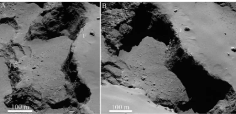
Fig. 5. Two views – A): NAC_2014-09-21T02.34.51.832Z_F41; and B): NAC_2014-09-22T02.34.52.186Z_F41 – used in this work. F marks an 80 m long fracture present on the cli↵ wall. Images were acquired from a distance of 30 km and have a resolution of 0.5 m/px.
That all cli↵s are smaller than this theoretical upper limit supports our choice of parameters. Our model shows that, given the right conditions, it is possible to grow or preserve cli↵s that are much larger that what we observe. We interpret the fact that most cli↵s are smaller than 100 m as an erosional e↵ect. Even if the cli↵ is structurally strong enough to support itself, the com-bination of local gas flows and thermo-mechanical stresses will greatly reduce the cohesion of the material. As active eroding processes and intrinsic weaknesses of the material (for instance pre-existing faults) are not taken into account in the simple model, they may very well explain our observations.
Indeed, high resolution images show that most cli↵s dis-play several types of fracturing patterns: polygonal features on the walls, which are characteristics of sublimation and ther-mal stresses; larger features of the cli↵ edge that likely lead to the slumping of material, for instance the 80 m long fracture marked in Fig.5. A review of fracturing on the nucleus of 67P is available inEl-Maarry et al.(2015a).
That cli↵s are collapsing is strongly supported by the ob-servation that most cli↵s present fallen debris at their foot. We decided to quantify this observation by performing a thorough boulder counting of the area in the proximity and below one of the major active cli↵s located at the border between the Seth and Hapi regions at the edge of the area also known as Landing Site Candidate A1.
We made use of two OSIRIS NAC images obtained on September 21 at 02:34:51UT and on September 22 at 02:34:52 UT. Both images have a similar resolution, 0.48 m/px for the first one and 0.49 m/px for the second one, since they were taken at 27.58 km from the comet nucleus center and 28.07 km, respectively. As we can see in Fig. 5, the two views, A and B, present unique observation geometries that give us the opportunity to analyze the boulder deposits located below the wall/cli↵ of Site A. Moreover, the high resolution provided by such images allows unambiguous identification of boulders bigger than 1.5 m. This value corresponds to the three-pixel sam-pling rule, which was chosen to minimize the likelihood of false detection (Nyquist 1928).
In Fig.6we show the reference image (A) used in this work and the two main units we have identified. Image (B) in the same figure shows the boulder counts for each unit. The talus unit is the area that is directly below the cli↵, while the distal detri-tal deposits is located about 100 m away from it. The division between the talus and the distal detrital deposit is based on the 1 http://www.esa.int/Our_Activities/Space_Science/ Rosetta/Rosetta_Landing_site_search_narrows
Fig. 6.Boulder statistics below one of the active cli↵s. PanelA): the two units, talus and the distal detrital deposits, identified for this work. PanelB): the location of the detected boulders, subdivided into di↵erent diameters. The di↵erence in sizes between boulders located below the cli↵ and those far from it is evident.
di↵erent geomorphological textures they show. The talus deposit is constituted by smaller boulders typically located below or in close proximity to the overlying cli↵. This finer material shows a homogeneous texture that is not recognizable in the distal detri-tal deposit. On the contrary, the disdetri-tal detridetri-tal deposit lies farther away from the cli↵, showing bigger boulders with a more het-erogeneous and articulated texture.
The complete boulder count of the area used the technique presented in Fig. 7 ofPajola et al.(2015). By manually identi-fying the boulders through the ArcGIS software, we measured their position in the surface of the comet, and assuming their shapes as circumcircles, we derived their maximum length, i.e. the diameter, and the corresponding area.
We identified a total number of 730 boulders, 657 of them satisfying the three-pixel sampling rule. The diameter of the 73 other boulders can be estimated from their cast shadows, but since their statistics are not complete, they cannot be consid-ered in this analysis. In Fig.6C, the location of such boulders is shown together with a color-coded size distribution. The number of boulders bigger than 1.5 m is 469 for the talus deposit and 188 for the distal detrital deposits.
A clear dichotomy can be observed between the sizes of the boulders that belong to the talus area and those that constitute the distal deposits (Fig.6, panel C). Indeed, while the boulders di-rectly below the cli↵ hardly reach 4 m in diameter, those that are farther out from it are frequently above this dimension, reaching in one case a value of 15 m. To quantify the power-law index of the boulder distributions, we plotted the cumulative number of boulders versus their size. The obtained results for both the talus and the distal detrital deposits are presented in Fig.7.
By fitting the plots of Fig. 7, we obtained two di↵erent power-law index for the two considered areas: –3.9 +0.2/–0.4 for the talus deposit, and –2.4 +0.2/–0.3 for the distal detrital de-posits. When comparing these two values, a steeper power-law index, as observed in the talus deposit, means that there is an increase in the population of smaller sized boulders with respect to the bigger ones. In contrast, a greater number of bigger boul-ders in the distal detrital deposits, coupled with fewer smaller boulders, has the main result of lowering the power slope index derived from the cumulative distribution.
These numbers should be compared to the global boulder size distribution on 67P presented in Pajola et al. (2015) for blocks greater than 7 m, as well as the boulder size distribution of debris at the bottom of active pits shown inVincent et al.(2015). These papers have shown that a power-law index of –3.9 falls inside the –3.5 to –4 range suggested for gravitational events triggered by sublimation and/or thermal fracturing causing re-gressive erosion. Despite di↵erences in sizes, this index seems
Fig. 7. Cumulative number of boulders computed for both the Talus and the Distal detrital deposits. The bin size here is 0.5 m, which is the resolution per pixel derived from the OSIRIS NAC images used. to confirm that the talus deposit we see below the cli↵ may well be the result of regressive erosion favored by sublimation from the cli↵ itself. Such a talus does not present bigger blocks as the detrital deposit does, because its margins are continuously refur-bished by blocks and grains from the nearby cli↵, as is the case for other pits and alcoves in Seth region. In contrast, the distal detrital deposits are generally characterized by bigger boulders than for the talus ones and by the presence of blocks smaller than 3 m. This is confirmed by the lower, –2.4 index, and a lower cumulative number of identified blocks, 188 versus 469. Since we have not yet detected a new boulder in these areas, it is not clear whether the larger blocks in the distal detrital deposit are actually related to the cli↵ erosion or if they stem from a com-pletely di↵erent process. Even in the low gravity of the comet, it seems unlikely that a >10 m diameter block could travel >100 m distance without breaking into smaller elements.
4.3.2. Granular flows
Mass wasting is observed close to the top edge of most active cli↵s, with a flow directed along the local slope. Some flows are visible in Fig. 5 (arched shapes in the dust layer on the cli↵ plateau). Figure 8 shows a few more examples of these avalanches at di↵erent places on the nucleus.
We calculated the slopes of these terrains taking the lo-cal gravity and centrifuge force into account. The gravity of the body is calculated on the polyhedral shape of the nucleus (Preusker et al. 2015), assuming a constant density of 500 kg m 3
(value fromSierks et al. 2015updated to the latest estimate of the comet volume). We find that slopes of granular flows vary from 20 to 30 . These slopes define the maximum angle of re-pose for cometary material, slightly below what is measured for granular material on rocky bodies (typical value of 30 ).
It is not obvious from our images whether these features are material shu✏ed around by local gas release or “dry” granular not triggered by a gas flow. We tend to favour the latter explana-tion because of the general good agreement between flow direc-tion, gravity, and size distribution of debris. In-place reorganiz-ing of dust would a↵ect only the smaller grains because the gas flows involved cannot push meter-sized debris down the cli↵s.
We propose that granular flows are triggered by the collapse of cli↵s. We do observe the edges of cli↵s slumping down in many places and losing blocks from erosion. At some point the dust mantle covering the cli↵ top is no longer supported on its edge and will start to flow down the local gravity vector (Fig.4).
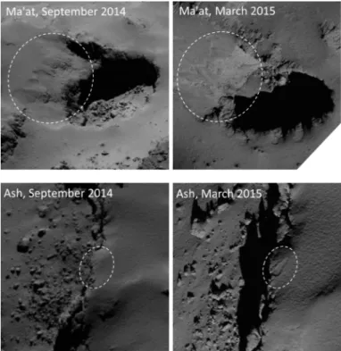
Fig. 8. Evolving flows observed in September 2014 and March 2015. Top panel: flows from Ma’at regions between two of the active pits have changed; their outline is di↵erent and they seem to have expanded laterally. Bottom panel: new flow in Ash region, following the partial collapse of one ac-tive cli↵. Image references for top panels: NAC_2014-09-12T01.33.04.375Z_ID30_1397549400_F22 & NAC_2015-03-28T16.18.50.365Z_ID10_1397549000_F82; and bottom pan-els: NAC_2014-09-10T18.34.00.345Z_ID30_1397549000_F22 & NAC_2015-03-28T14.19.49.405Z_ID10_1397549000_F82).
We have observed a few examples of cli↵ edges about to col-lapse, with blocks appearing to be almost separated from the cli↵ by a large crack. These blocks typically extend 10 m from the cli↵ edge, a size comparable to the maximum size of blocks at the cli↵’s foot. We propose this scale as the maximum dis-tance fractures can propagate inside the cli↵ before triggering the collapse.
If a cli↵ is active, we expect this process to be ongoing. The sublimation and release of volatiles from the cli↵ will further its weakening and generate new collapses with local retreats of 10 m or more. Granular flows and other mass wasting previ-ously formed will be reactivated or modified subsequently, and we should be able to observe their evolution. Collapsing cli↵s will also form new flows. This is challenging to measure because many changes are at the limit of our detection capabilities, but we have observed evolving flows in a few areas, as is consistent with the model. See examples in Fig.8.
4.3.3. Exposure of bright material
The sources associated to activity, more exactly cli↵s and col-lapsed wall features, are consistently associated to specific var-iegation. Edges of cli↵s are a few percent brighter and bluer than inactive surfaces. This is true in both the visible (Fornasier et al. 2015;Oklay et al. 2015) and infrared ranges of the spectra (Capaccioni et al. 2015).
In addition, more than a hundred very bright spots have been observed on the comet, most of them appearing as clusters in
the debris field of active cli↵s. They are interpreted as water ice exposed on the surface of boulders dislocated from the cli↵ dur-ing collapse (Pommerol et al. 2015).
We use this observational fact to partially reevaluate what the source of jets actually is. As explained in Sect.2.2, our jet obser-vations often do not sample the first few 10 s of meters above the surface, and the link between jet and cli↵ is only an extrapola-tion of the jet direcextrapola-tion measured above this blind spot. It is very possible that the real active spot extends beyond the cli↵ itself and includes the debris at the cli↵ foot, as well as the bright ma-terial newly exposed in mass-wasted areas. The gas flows arising from all these features will compete against each other and the topography, leading to a focused jet. This can explain why dust jets starting from vertical surfaces seem to bend upward rapidly and finally expand radially away from the nucleus. It can be that the jet direction is fully controlled by morphological features, such as fractures, but it is more likely that the jet is pushed up-ward by gas arising from the debris field at the bottom of the cli↵. This case is compatible with the work of several authors who studied the trajectories of gas flows around complex topo-graphic features (Crifo et al. 2002;Skorov et al. 2006;Vincent et al. 2012).
Can the variegation of the talus like the one seen in Fig.2
be explained by airfall material ejected from the cli↵? The bluer debris field typically extend 100 to 150 m from the cli↵s. Simple ballistic considerations show that this distance is reached by ma-terial ejected at a speed of at most 15 cm s 1, which is ten times
less than the escape velocity (1 m s 1) and 50 times less than
the typical velocity of dust particles ejected from the surface (3.75 m s 1,Rotundi et al. 2015). Because we see the jet
ma-terial escaping from these areas, it is unlikely that a significant fallback takes place, and it seems more probable that the var-iegation is due to intrinsic properties of the fallen blocks. As a significant portion of their surface was not exposed to the Sun when they were still attached to the cli↵, it seems logical that they contain more volatile material than the surrounding terrains. 4.4. Theoretical model
Most jets from the northern hemisphere of 67P arise from areas with sharp topography, in particular cli↵s. We have discussed the observational evidence for the regressive erosion that may be triggered by the activity. The following paragraphs will review how these typical morphologies can help sustaining the activity. If fractures act as nozzle for the gas flows, e↵ectively leading to the formation of jets, it means that they also define the small-est possible jets. All missions to comets have resolved jets as small as the spatial scale of their observations, pushing down the lower limit but not fixing it. The good correlation between jets and fractured terrains, on one hand, and the smallest jet diameter and fracture width in these areas, on the other, suggest that the smallest jets we observe are constrained by the fracture dimen-sions, a couple of meters wide at most. Because jets are fuzzy, and more than one fracture is active in any area, jets often ap-pear to arise from a few fractures rather than from a single one. The idea of jets arising from cracks, holes, or other morphologi-cal features has been extensively discussed in several papers: for instance,Belton(2013),Bruck Syal et al.(2013) for comets, or
Yeoh et al.(2015), who modeled such phenomena to explain the water plumes of Enceladus.
A detailed modeling of the gas dynamics and dust accelera-tion within the fractures requires complex simulaaccelera-tions and will be the subject of a future study. Instead, we present here some
physical considerations that approximate the real processes tak-ing place in these fractures.
The main constraint on our problem is that gas flows in the jets must be able to lift the dust grains that other instruments have collected around the comet. These grains are quite large for comet standards. Indeed, light scattering properties in the ground-based observations of 67P are dominated by 100 µm size particles, and both GIADA and COSIMA onboard Rosetta show a lack of micron-sized grains (Rotundi et al. 2015;Schulz et al. 2015). Dust velocities are measured by GIADA (Rotundi et al. 2015). The cumulative distribution shows a mean velocity equal to 3.75 m s 1, '4 times the escape velocity. The average dust
density is 1900 kg m 3.
Once a particle is released, drag force and gravity are the main forces that will control its trajectory. Other e↵ects like ra-diation pressure are negligible as long as the dust motion is still coupled to the gas, which is the case for the short time and dis-tance scales we consider here.
Nucleus gravity is calculated from the OSIRIS volume reconstruction (21.4 km3) and the Rosetta Radio Science
Investigation mass estimate (1 ⇥ 1013kg), both values published
inSierks et al.(2015). We assume homogeneous density at first order. The average mean radius is 1720 m, and the average sur-face gravity is 2.25 ⇥ 10 4m s 2. We use a simple aerodynamic
model to calculate the drag force, assuming spherical particles and a gas molecule free mean path that is much smaller than the dust diameter:
Fd=12⇢gv2rCdA (N), (2)
with ⇢g the gas density, vr the relative velocity of the gas with
respect to the particle, A the cross section of the particle, and Cd
the drag coefficient ('1 for roughly spherical grains). Because vdust⌧ vgas, we can replace vrwith vgasin the equation.
We have not considered complex situations with gas perco-lating through a porous dust layer. We rinstead assume a subli-mating source inside a fracture or at the bottom of a wall and look at how the arising gas flow could tear out dust grains in its vicinity.
Dust can only be lifted if the drag force overcomes grav-ity and additional forces holding the particle in place. These forces are not characterized well for cometary material but can be approximated using the surface tensile strength.Thomas et al.
(2015),Vincent et al.(2015), andGroussin et al.(2015) have in-dependently estimated the tensile strength of the surface upper layers in various regions by studying the morphology of pits and overhangs and reached the same average value of Y = 50 Pa.
We consider a spherical particle half embedded in the nu-cleus surface. The tensile force holding the particle in place is Ft=Y ⇥ area = 50 ⇥ ⇡r2(N) and is typically five orders of
mag-nitude greater than the weight of the particle. One could also consider cohesion or shear strength instead of tensile strength, but the order of magnitude is similar.
The drag force is a function of particle size + gas pressure and velocity. A gas expanding from a flat surface would have a mean velocity purely driven by thermal consideration. The Maxwellian distribution gives the root mean squared speed: vgas=
r 3kBT
m (m s 1) (3)
with kBBoltzmann’s constant, and m the molecular mass of H2O
(3 ⇥ 10 26kg).
The gas density is defined by
Table 1. Gas dynamics and drag force as a function of grain size and temperature. T (K) v(m s 1) Psat (Pa) ⇢
gas(kg m3) Fdrag (N) Fdrag (N) Fdrag (N) Fdrag (N)
170 484.36 6.88E-04 5.10E-07 4.48E-14 4.48E-12 4.48E-10 4.48E-08
180 498.40 5.10E-03 3.58E-06 3.33E-13 3.33E-11 3.33E-09 3.33E-07
190 512.05 3.07E-02 2.04E-05 2.00E-12 2.00E-10 2.00E-08 2.00E-06
200 525.36 1.54E-01 9.78E-05 1.01E-11 1.01E-09 1.01E-07 1.01E-05
210 538.33 6.64E-01 4.02E-04 4.33E-11 4.33E-09 4.33E-07 4.33E-05
220 551.00 2.51E+00 1.45E-03 1.63E-10 1.63E-08 1.63E-06 1.63E-04
230 563.38 8.43E+00 4.68E-03 5.49E-10 5.49E-08 5.49E-06 5.49E-04
250 587.37 7.12E+01 3.66E-02 4.64E-09 4.64E-07 4.64E-05 4.64E-03
260 599.00 1.83E+02 9.05E-02 1.19E-08 1.19E-06 1.19E-04 1.19E-02
270 610.41 4.38E+02 2.09E-01 2.86E-08 2.86E-06 2.86E-04 2.86E-02
280 621.61 9.87E+02 4.55E-01 6.43E-08 6.43E-06 6.43E-04 6.43E-02
290 632.61 2.10E+03 9.38E-01 1.37E-07 1.37E-05 1.37E-03 1.37E-01
300 643.43 4.25E+03 1.84E+00 2.77E-07 2.77E-05 2.77E-03 2.77E-01
Particle size 1 µm 10 µm 100 µm 1000 µm
Tensile force (N) 1.96E-11 1.96E-09 1.96E-07 1.96E-05 with R = 8.31447 (constant for perfect gases).
The vapor pressure of ice can be defined as a function of temperature, which is usually defined empirically. Reviews of various models and experimental measurements are available in
Andreas(2007) andGundlach et al.(2011). In this paper we use the empirical relation:
Psat(T) = a1e a2/T (Pa) (5)
with a1 = 3.23 ⇥ 1012 Pa and a2 =6134.6 K (Gundlach et al.
2011). Using these equations we can calculate the drag force as a function of the temperature. Results for di↵erent grain sizes are summarized in Table1.
This simple modeling approach highlights that we need to overcome a certain cohesive force to lift up dust parti-cles: for instance, 1.96 ⇥ 10 7 N for particles of 100 µm.
This typically corresponds to a sublimation temperature higher than 205 K. Figure9shows how this minimum necessary tem-perature evolves with respect to the tensile strength of the sur-face. Within the assumptions described above it can be fitted by a power law:
Tmin =181 ⇥ Y0.0334 (K). (6)
This function describes only a lower limit for the gas flow needed to lift up dust particles. One must be aware of a few limitations to our model:
– We do not know the tensile strength of the surface’s upper layers, but only have estimates for layers that are a few tens of meters thick. The actual cohesion of the top surface may be much higher, especially in the presence of organic mate-rials that can act as a glue between the grains, because of the sintering caused by the many thermal cycles that took place on the surface.
– We used Stokes’ equation to calculate the drag force. If the mean free path of the gas is much greater than the size of the particle, we must instead consider Epstein’s model, which e↵ectively reduces the efficiency of the drag force (Blum 2006). In practice, this is equivalent to replacing v2
r by vrvgas
in Eq. (2). Because vdust⌧ vgasin our case, both regimes lead
to similar drag forces.
– In our model drag force and cohesion vary with the surface of the particle, i.e. the square of its radius, therefore the ratio of drag force and cohesion is independent of the particle size.
Fig. 9.Minimum sublimation temperature needed to produce a gas flow able to tear o↵ dust grains that are half embedded in the nucleus, as a function of the tensile strength of the surface.
– The pressure we calculate is only valid very close to the source. As gas expands in the vacuum, the pressure drops rapidly, reducing the drag force away from the source. – In addition, there may be an existing ambient pressure that
may reduce the efficiency of the newly created gas flow, al-though it will allow a stronger collimation.
We therefore expect the real flux necessary to lift up the dust to be even larger than the limit we calculated earlier, which means that either the surface needs to reach an even higher tempera-ture or that other mechanisms will focus the gas flow and help it provide a much stronger drag force.
The limiting factor to reaching such a relatively high subli-mation temperature is the available thermal energy. The major contributor in the energy balance of cometary surface crusts is solar irradiation. Owing to the low thermal inertia of these crusts and the nearly instantaneous thermal re-emission, comparably high sublimation rates in deeper crust layers are hardly reached. Morphologic structures, such as cracks, fractures, or holes, are more likely to enhance the sublimation rate at deeper depths of the crust, because they prevent large amounts of heat being re-emitted into space. These structures act as heat traps when under
favorable illumination conditions and generating higher average temperatures and thus higher sublimation rates. They will, how-ever, be heated only for a short time, and therefore sustaining jets from a given area will require a fracture field with di↵erent fracture orientations with respect to the Sun. This is indeed what we observe in the pits in Seth region (Vincent et al. 2015): the large jet arising from a pit is composed of small features sequen-tially activated as di↵erent fractured areas of the walls become illuminated (typically only for a couple of hours).
The narrow geometry of fractures not only describes a heat trap, but from the point of view of gas dynamics is also similar to a pipe or a nozzle. Once released, the gas cannot expand in all directions, but its flow is constrained by the geometry of its sur-roundings. Depending on the temperature of the fracture walls, we can have a slight cooling or warming of the gas, but overall it is likely that the fracture will accelerate the flow, hence increas-ing the e↵ective drag force. Such a mechanism is described, for instance, in Yeoh et al. (2015). We instead expect a warming when the walls are inert; sublimation at the fracture wall will lead to slightly colder gas temperatures.
Of course, this description is highly speculative since we cannot constrain the real fracture geometries from the current data, but the fact that we see enhanced gas or dust flows over these fractured areas makes this process plausible. Constraining this e↵ect further will require detailed theoretical and experi-mental modeling. We refer the reader to Hoefner et al. (in prep.) for advanced numerical studies of thermophysical conditions in cometary fractures, and implications on the activity.
4.5. A general mechanism? Comparison with other comets When compared at similar spatial scales, the Jupiter family comets visited by spacecrafts are quite similar. They have com-parable size, albedo, and large scale morphology. Activity oc-curs at similar levels and even outbursts are comparable in their amount of ejected material (Belton 2013;Tubiana et al. 2015). Therefore why would the erosion mechanism presented in pre-vious sections not take place on other comets as well? There is little evidence that this is indeed the case.
Comets 81P/Wild 2 and 9P/Tempel 1 have both been ob-served by space missions at similar resolutions (10 m/px). Both missions followed the comets’ activity during their encounter, and traced jets back to regions of the surface (Sekanina et al. 2004;Farnham et al. 2007,2013). Although the lower resolution and limited time coverage did not allow for a jet reconstruction that is as precise as the one we obtained with 67P, many jets were consistently linked to rough terrains. In particular for 81P, many jets were seen arising from within or on the edge of local depres-sions, which is quite similar to what we see in the Seth region on 67P. Pits on 81P are typically shallower than on 67P, which has been interpreted as evidence of erosion and infill (see discus-sion inVincent et al. 2015). On 9P, many jets were linked to a ragged area bordering a large smooth terrain and, in particular, to the scarped edge of this terrain (Farnham et al. 2007). This area, however, has been imaged in two consecutive orbits by the mis-sions Deep Impact (in 2005) and Stardust-NExT (in 2011). Both flybys happened around perihelion passage and imaged the same area of the comet with similar illumination, thus providing the best conditions to detect surface changes. Indeed,Thomas et al.
(2013) reports a significant retreat of the cli↵ up to 50 m in some areas, as well as the lateral expansion of surface depressions in the vicinity and putatively linked this evolution to the ongoing activity. Although some uncertainty uncertainty remains as to where the source of these jets really lies (smooth patch itself?
cli↵? talus?), we know for a fact that erosion took place in this area between 2005 and 2010 (deep impact and stardust encoun-ters) even if this region was no longer a source of jets in the second encounter (Farnham et al. 2013).
In retrospect, it seems the findings on 81P and 9P are similar to what we observe on 67P at higher resolution. The di↵erent scale of changes is likely due to the di↵erence in insolation for both comets. Even if the smooth patch of comet 9P was only illuminated for a fraction of the rotation and at shallow angle, the receding edge would have been facing the Sun directly for a short while, receiving about 600 W m 2of solar energy.
On the other hand, cli↵s in 67P’s Seth region are in po-lar winter at perihelion and are not very illuminated below an heliocentric distance of 3 AU, thus receiving an irradiance of at most 150 W m 2. In addition to that, these areas experience
strong shadowing because they are located close to the bottom of the largest concavity of the nucleus and are therefore illuminated only for a few hours instead of continuously for Tempel 1. This leads to a maximum erosion of only 1 m (Keller et al. 2015), and therefore strong changes will only occur through sudden events (like a block falling from the scarp) rather than continuous erosion.
5. Conclusions
The high resolution observations of dust jets arising from the nu-cleus of comet 67P from August 2014 to May 2015 led us to pro-pose a new scenario to explain both the formation of cometary jets and the presence of erosional features seen on many comets. Our findings can be summarized as follows:
– Seasonal and diurnal variations of activity in the northern hemisphere of comet 67P are correlated well with solar illu-mination, hence linked to volatile sources within the diurnal thermal skin depth of the surface.
– We presented observational evidence that northern jets arise in the majority from rough terrains rather than smooth areas, more specifically from fractured walls.
– We interpret this activity as a combination of meter-scale jets accelerated in fractures, and decameter scale flows arising from the mass wasted brighter debris at the cli↵ foot. – Our findings imply that erosion of the comet surface
primar-ily takes place along these active cli↵s, and therefore they should be showing the most significant changes, some of them already observed.
– Activity-driven erosion of cli↵s occurs in many places on 67P and may have been observed on 9P and 81P. We propose that this is a general process taking place on all comets. The process described above is very general and describes one type of activity that explains most active sources of the north-ern hemisphere of 67P. It is important to keep in mind that other types of activity may arise, and our classification of ac-tive sources is still a work in progress. As the comet approaches perihelion, we keep monitoring the activity and will investigate how jets and sources behave at closer heliocentric distance. We do expect to observe other types of activity; for instance, previ-ously insulated area may receive enough solar energy to allow the sublimation of volatiles without the need for specific terrain morphology.
Acknowledgements. OSIRIS was built by a consortium led by the Max Planck Institut für Sonnensystemforschung, Göttingen, Germany, in collaboration with CISAS, University of Padova, Italy, the Laboratoire d’Astrophysique de Marseille, France, the Instituto de Astrofisica de Andalucia, CSIC, Granada,
Spain, the Scientific Support Office of the European Space Agency, Noordwijk, The Netherlands, the Instituto Nacional de Tecnica Aeroespacial, Madrid, Spain, the Universidad Politecnica de Madrid, Spain, the Department of Physics and Astronomy of Uppsala University, Sweden, and the Institut für Datentechnik und Kommunikationsnetze der Technischen Universität Braunschweig, Germany. The support of the national funding agencies of Germany (DLR), France (CNES), Italy (ASI), Spain (MINECO), Sweden (SNSB), and the ESA Technical Directorate is gratefully acknowledged. We thank the Rosetta Science Ground Segment at ESAC, the Rosetta Mission Operations Centre at ESOC and the Rosetta Project at ESTEC for their out-standing work enabling the science return of the Rosetta Mission. We thank the anonymous reviewers for their constructive criticism and support of our findings.
References
Acton, C. H. 1996,Planet. Space Sci., 44, 65
Alí-Lagoa, V., Delbo’, M., & Libourel, G. 2015,ApJ, 810, L22
Andreas, E. L. 2007,Icarus, 186, 24
Belton, M. J. S. 2010,Icarus, 210, 881
Belton, M. J. S. 2013,Icarus, 222, 477
Blum, J. 2006,Adv. Phys., 55, 881
Brownlee, D. E., Horz, F., Newburn, R. L., et al. 2004,Science, 304, 1764
Bruck Syal, M., Schultz, P. H., Sunshine, J. M., et al. 2013,Icarus, 222, 610
Capaccioni, F., et al. 2015, Science, submitted
Crifo, J.-F., Rodionov, A. V., Szegö, K., & Fulle, M. 2002,Earth Moon and Planets, 90, 227
El-Maarry, R., Thomas, N., Gracia-Beraá, A., et al. 2015a,Geophys. Res. Lett., 42, 5170
El-Maarry, R., Thomas, N., Giacomini, L., et al. 2015b,A&A, 583, A26
Farnham, T. L., Wellnitz, D. D., Hampton, D. L., et al. 2007,Icarus, 187, 26
Farnham, T. L., Bodewits, D., Li, J.-Y., et al. 2013,Icarus, 222, 540
Feaga, L. M., A’Hearn, M. F., Sunshine, J. M., Groussin, O., & Farnham, T. L. 2007,Icarus, 190, 345
Fornasier, S., Hasselmann, H., Barucci, M. A., et al. 2015,A&A, 583, A30
Groussin, O., Jorda, L., Auger, A.-T., et al. 2015,A&A, 583, A32
Gulkis, S., Allen, M., von Allmen, P., et al. 2015,Science, 347, 709
Gundlach, B., Skorov, Y. V., & Blum, J. 2011,Icarus, 213, 710
Keller, H., Knollenberg, J., & Markiewicz, W. 1994, Planet. Space Sci., 42, 367 Keller, H. U., Barbieri, C., Lamy, P., et al. 2007,Space Sci. Rev., 128, 433
Keller, H., Mottola, S., Davidsson, B., et al. 2015,A&A, 583, A34
Knollenberg, J., Lin, Z. Y., Hviid, S.F., et al. 2016, A&A, submitted
Lara, L. M., de León, J., Licandro, J., & Gutiérrez, P. J. 2005,Earth Moon and Planets, 97, 165
Lara, L. M., Lin, Z.-Y., Rodrigo, R., & Ip, W.-H. 2011,A&A, 525, A36
Lara, L. M., Lowry, S., Vincent J. B., et al. 2015,A&A, 583, A9
Lin, Z.-Y., Ip, W.-H., Lai, I.-L., et al. 2015,A&A, 583, A11
Melosh, H. J. 2011, Planetary surface processes (Cambridge Press)
Nyquist, H. 1928,Transactions of the American Institute of Electrical Engineers, 47, 617
Oklay, N., Vincent, J.-B., Sierks, H., et al. 2015,A&A, 583, A45
Pajola, M., Vincent, J.-B., Güttler, C., et al. 2015,A&A, 583, A37
Pommerol, A., Thomas, N., El-Maarry, M. R., et al. 2015,A&A, 583, A25
Preusker, F., Scholten, F., Matz, K.-D., et al. 2015,A&A, 583, A33
Rotundi, A., Sierks, H., Della Corte, V., et al. 2015,Science, 347, 3905
Schulz, R., Hilchenbach, M., Langevin, Y., et al. 2015,Nature, 518, 216
Sekanina, Z., Brownlee, D. E., Economou, T. E., Tuzzolino, A. J., & Green, S. F. 2004,Science, 304, 1769
Shi, X., Hu, X., Sierks, H., et al. 2016,A&A, 586, A7
Sierks, H., Barbieri, C., Lamy, P. L., et al. 2015,Science, 347, 1044
Skorov, Y. V., Markelov, G. N., & Keller, H. U. 2006,Sol. Syst. Res., 40, 219
Thomas, P., A’Hearn, M., Belton, M. J. S., et al. 2013,Icarus, 222, 453
Thomas, N., Sierks, H., Barbieri, C., et al. 2015,Science, 347, 440
Tozzi, G. P., Patriarchi, P., Boehnhardt, H., et al. 2011,A&A, 531, A54
Tubiana, C., Snodgram, C., Bertini, I., et al. 2015,A&A, 573, A62
Vincent, J.-B., Böhnhardt, H., & Lara, L. M. 2010,A&A, 512, A60
Vincent, J.-B., Sierks, H., Rose, M., & Skorov, Y. 2012, inEur. Planet. Sci. Congress, 358
Vincent, J.-B., Lara, L. M., Tozzi, G. P., Lin, Z.-Y., & Sierks, H. 2013,A&A, 549, A121
Vincent, J.-B., Bodewits, D., Besse, S., et al. 2015,Nature, 523, 63
Yeoh, S. K., Chapman, T. A., Goldstein, D. B., Varghese, P. L., & Trafton, L. M. 2015,Icarus, 253, 205
1 Max-Planck Institut fuer Sonnensystemforschung, Justus-von-Liebig-Weg, 3 37077 Goettingen, Germany
e-mail: [email protected]
2 Centro di Ateneo di Studi ed Attivitá Spaziali “Giuseppe Colombo” (CISAS), University of Padova, via Venezia 15, 35131 Padova, Italy 3 Institute for Geophysics and Extraterrestrial Physics, TU
Braunschweig, 38106 Braunschweig, Germany
4 Department of Physics and Astronomy “G. Galilei”, University of Padova, Vic. Osservatorio 3, 35122 Padova, Italy
5 Aix-Marseille Université, CNRS, LAM (Laboratoire d’Astro-physique de Marseille) UMR 7326, 13388 Marseille, France 6 Centro de Astrobiologia (INTA-CSIC), European Space Agency
(ESA), European Space Astronomy Centre (ESAC), PO Box 78, 28691 Villanueva de la Canada, Madrid, Spain
7 International Space Science Institute, Hallerstrasse 6, 3012 Bern, Switzerland
8 Research and Scientific Support Department, European Space Agency, 2201 Noordwijk, The Netherlands
9 Department of Physics and Astronomy, Uppsala University, Box 516, 75120 Uppsala, Sweden
10 PAS Space Research Center, Bartycka 18A, 00716 Warszawa, Poland
11 Department for Astronomy, University of Maryland, College Park, MD 20742-2421, USA
12 Gauss Professor Akademie der Wissenschaften zu Göttingen, 37077 Göttingen, Germany
13 LESIA, Observatoire de Paris, CNRS, UPMC Univ. Paris 06, Univ. Paris-Diderot, 5 place J. Janssen, 92195 Meudon Principal Cedex, France
14 LATMOS, CNRS/UVSQ/IPSL, 11 boulevard d’Alembert, 78280 Guyancourt, France
15 INAF Osservatorio Astronomico di Padova, Vicolo
dell’Osservatorio 5, 35122 Padova, Italy
16 CNR-IFN UOS Padova LUXOR, via Trasea 7, 35131 Padova, Italy 17 Department of Industrial Engineering University of Padova via
Venezia, 1, 35131 Padova, Italy
18 University of Trento, via Sommarive, 9, 38123 Trento, Italy 19 Physikalisches Institut, Sidlerstrasse 5, University of Bern, 3012
Bern, Switzerland
20 INAF–Osservatorio Astronomico di Trieste, via Tiepolo 11, 34143 Trieste, Italy
21 Instituto de Astrofisica de Andalucia-CSIC, Glorieta de la Astronomia, 18008 Granada, Spain
22 Institute of Planetary Research, DLR, Rutherfordstrasse 2, 12489 Berlin, Germany
23 Institute for Space Science, National Central University, 32054 Chung-Li, Taiwan
24 Budapest University of Technology and Economics, Department of Mechatronics, Optics and Engineering Informatics, Muegyetem rkp 3, 1111 Budapest, Hungary
25 ESA/ESAC, PO Box 78, 28691 Villanueva de la Cañada, Spain 26 Centre for Astrophysics and Planetary Science, School of Physical
Sciences, The University of Kent, Canterbury CT2 7NH, UK 27 Department of Information Engineering, University of Padova, via
Gradenigo 6/B, 35131 Padova, Italy
28 Observatory of the Hungarian Academy of Sciences, PO Box 67, 1525 Budapest, Hungary
Appendix A: Additional figures
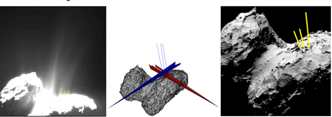
Fig. A.1.Summary of the direct inversion technique. Left panel: jets are identified in two di↵erent images, only one is shown here, see Fig.A.2 for the full sequence. Middle panel: triangulation, for each image we know the precise position and attitude of the spacecraft. From this we define the planes of jets (spacecraft, line of sight, observed jet direction). The intersection between these planes defines the jet in three dimensions, and we calculate their intersection with the surface. Right panel: knowing sources and directions, plus some assumptions on grain velocity, we can reconstruct the jets trajectories (yellow lines).
Fig. A.2.Ten WAC images from a sequence acquired on 10 September 2014 from a distance of 29 km and a sub-spacecraft latitude of +48 . The sequence shows the diurnal variation of activity over 9 h (72%) of nucleus rotation. Each view is separated from the previous one by about 1 h (30 of nucleus rotation). The Sun and the comet’s north pole are pointing up in these images. Brightness levels are stretched linearly to emphasize the 5% least bright pixel values.
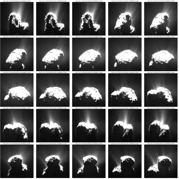
Fig. A.3.25 WAC images from a sequence acquired on 22 November 2015 from a distance of 29 km and a sub-spacecraft latitude of –57 . The sequence shows the diurnal variation of activity over 10.8 h of rotation (88% of the total period). Each view is separated from the previous one by about 20 min (10 of nucleus rotation). There is a gap of 2 h between the fourth and last rows and after the last image due to spacecraft navigation slots. The Sun and the comet’s north pole are pointing up in these images. Brightness levels are stretched linearly to emphasize the 5% least bright pixel values.
Fig. A.4.25 NAC images from a sequence acquired on 12 April 2015 from a distance of 149 km and a sub-spacecraft latitude of –48 . The sequence shows the diurnal variation of activity over a full period. Each view is separated from the previous one by about 30 min (15 of nucleus rotation). There is a four-hour gap between the last two observations. The Sun and the comet’s north pole are pointing up in these images. Brightness levels are stretched linearly to emphasize the 5% least bright pixel values.
Fig. A.5.Maps of active sources obtained at three di↵erent epochs. From top to bottom: september 2014, November 2014, April 2015. The map is shaded according surface slopes, accounting for gravity and centrifugal force. White is flat, black is a vertical wall. The yellow line marks the subsolar latitude. These maps are not an exhaustive catalog of all sources, see Sect.3