Optimization of Ideal Solar Sails Earth Escape Trajectories using Dynamic Programming

(1)

A mio padre, mia madre e mia sorella

(2)

Abstract

Solar sails have long been seen as an attractive concept for low-thrust propulsion. Due to their no-need of fuel, solar sailing is becoming, with growing interest, object of further research for high-energy missions. One of the most important tasks, during the feasibility analysis and preliminary design of a deep space mission, is the design and optimization of the interplanetary transfer trajectory. The search of minimum time escape trajectories from Earth gravitational field appears to be the first step in such a study. In this thesis work, the continuous time, space and control optimization problem of finding near-minimum time Earth escape trajectories for a solar sail, has been discretized in order to exe-cute the Dynamic Programming algorithm. A performance index that permits to achieve escape, from the analyzed starting orbits, is set up; afterwards an optimization using the DP algorithm is carried out, producing an improvement in terms of time to escape, even if small, with respect to the performance index initial guess solution. Two dimensional trajectories lying onto the ecliptic plane are investigated, using the ideal solar sail model. A characteristic sail accelera-tion of 1 mm/sec2_{is considered, neglecting all secondary perturbation effects on}

the sail. Trajectories are generated starting from two initial orbits of practical interest: a Geosynchronous orbit and a GTO. Trajectories and times to escape are compared with results obtained through another near-optimal method, such as the one that maximizes the instantaneous rate of increase of total orbital energy, largely used nowadays.

(3)

Acknowledgements

I would like to express my sincerest appreciation to Prof. Emilio Frazzoli, advi-sor and friend, without whom my wonderful experience in Champaign-Urbana would have never been possible. Many thanks to Prof. Giovanni Mengali and to Dr.Eng. Alessandro Quarta as well, for their suggestions in the final drafting of my thesis.

(4)

Ringraziamenti

Vorrei ringraziare tutte le persone che mi sono state vicino in questi anni di Universitá. Vorrei qui ricordare gli amici di Vieste a cui sono piú legato, a partire da quelli con i quali ho condiviso i momenti piú spensierati e belli, dall’infanzia fino ad oggi: Libero, Nicola L., Alessio, Lino, Roberto, Giacomo, Nicola B., Michele S., Nicola F., Marco S., Marco M., Elio. Gli amici del karate: Adriano, Salvatore, Danilo e Antonio R.. Poi i miei cari amici del Liceo: Giuseppe L., Antonio M., Antonio L., Pino, mio cugino Giuseppe T.. Gli amici dei primi anni dell’Universitá: Pasquale, Gilberto, Domenico, Samuel. Con loro ho condiviso momenti indimenticabili. Infine, i miei amici Valerio e Nicola, a cui sono legato da profonda amicizia, le persone che piú di tutte ci sono state negli ultimi due anni, nei momenti belli, ma anche, e soprattutto, in quelli meno facili. Ricordo con affetto tutte le persone che ho conosciuto a Champaign, a partire dai miei compagni di casa: Carlos, Richard e Jon, gli amici dell’associazione degli italiani a Champaign, e Francesco N..

(5)

Introduction

Solar sails directly use solar radiation pressure on a large reflecting surface to obtain low-thrust propulsion. They are like big and light mirrors that reflect beams of radiation. The physics behind the concept is straightforward: photons carry momentum as well as energy, and so electromagnetic radiation, including sunlight, exerts a force on any surface it illuminates. It follows that the main characteristic of a solar sail is the no need of fuel.

Although only capable of very low thrust, solar sails operate continuously over indefinitely long periods, the only limitation being the materials strength, and using a free inexhaustible form of energy, they can provide, over long peri-ods, energy changes greater than are possible with either ion or chemical pro-pellants. Solar sails are, therefore, especially attractive for small mass inter-planetary missions, becoming competitive with respect to traditional propulsion systems.

1.1 Motivation

Traditionally, solar sailcraft trajectories are optimized by the application of numerical optimal control methods that are based on the calculus of variations. The convergence behavior of these optimizers depends strongly on an adequate initial guess, which is needed before optimization. In general the difficulty regarding the convergence to an optimal solution is increased by the scarce sensibility of the flight time with respect to small variations on the sail control vector. Therefore, depending on the difficulty and complexity of the problem, finding an optimal solar sailcraft trajectory usually turns into a time-consuming task that involves a lot of experience and expert knowledge in control theory

(9)

Figure 1.1: Square solar sail

and in astrodynamics. Even if convergence is achieved by the optimizer, the optimal trajectory is typically close to the initial guess that is usually far from the (unknown) global optimum. Moreover the numerical integration of the Boundary Value Problem (BVP) associated to the variational problem can be executed only for one initial orbit at time.

In this work a problem with continuous time, state and control, such as the solar sail escape problem, has been discretized in order to execute the Dynamic Programming algorithm. Dynamic programming leads to a globally optimal so-lution as opposed to variational techniques, for which this cannot be guaranteed in general. The initial guess of the performance index, calculated over an en-tire domain of states (orbits), will be found using a control law that maximizes the finite variation of specific orbital mechanical energy, as it will be described, between states in succession, owning to discretized escape trajectories. The op-timized performance index, will be an absolute minimum since a direct search is made, based on the principle of optimality. But this optimized performance in-dex will also be an approximate evaluation of the cost-to-go, and it will produce a sub-optimal policy for the original continuous problem due to interpolation. Therefore a prerequisite for success of this type of discretization is consistency. Continuity of cost-to-go functions may be sufficient to guarantee consistency even if the optimal policy is discontinuous in the state. This means that the optimal cost of the original continuous problem should be achieved in the limit

(10)

as the discretization becomes finer and finer.

It has been thought to implement a method of optimization, such as dynamic programming, to get an optimal performance index over an entire domain of states, and use the optimized performance index, to propagate optimal escape trajectories, choosing at each temporal step, the control value that minimizes the performance index.

1.2 Objectives

The purpose of this thesis work is to set up a technique to propagate (near) minimum time solar sail trajectories using a performance index, optimized by dynamic programming. The study involves five steps:

1. Choice of a set of classical orbital elements to define the state of the sailcraft during escape

2. Analytical integration over one orbit of the vectorial differential equations of the variation of parameters method, obtaining algebraic variation equa-tions that will be used as state equaequa-tions

3. The calculation of a performance index first guess, maximizing the varia-tion of specific orbital mechanical energy at each node of the discretized trajectories for a whole domain of initial orbits, using the integral variation equations previously found

4. The optimization of the performance index found, using the dynamic pro-gramming (DP) algorithm

5. The propagation of escape trajectories using the dynamic programming optimized performance index, making comparison with respect to trajec-tories obtained from the maximization of variation of total orbital energy strategy (over discretized trajectory), and trajectories produced by maxi-mization of instantaneous rate of total orbital energy control law (contin-uous trajectory)

1.3 Models and Hypothesis used in the Work

Here we report the main physical models and simplifying hypothesis used during this work, whose details, for some of them, will be afterwards given.

1. The ideal solar sail model is assumed; the sail is dynamically treated as point mass

(11)

2. Two-body gravity model is assumed with the gravitational effects of ter-tiary bodies, such as the Sun, neglected

3. Atmospheric drag over Low Earth Orbit (LEO) and shadowing effects of the Earth are neglected

4. Spherical Earth gravitational field is assumed (Earth oblateness neglected) 5. A circular orbit is assumed for the Earth; therefore the 6% variation in the magnitude of the solar flux due to the eccentricity of the Earth orbit, is not included

6. Small magnitude of the sail characteristic acceleration is assumed, result-ing in a very small net change in specific orbital mechanical energy over each orbit. As consequence, orbital parameters variations are considered small on temporal intervals appropriately selected.

7. Two-dimensional escape trajectories lying onto the ecliptic plane are in-vestigated

1.4 Literature Review

In this section we will try to delineate the state of the art. This review in-volves: first, the solar sails in general; second, the solar sails physical models; third, giving a background of solar sails trajectories optimization; and finally outlining a background of Dynamic Programming in optimal control problems for aerospace applications.

1.4.1 The Solar Sail Concept through the XX

th

_Century

The concept of the solar sail goes back far as 1924 to Tsiolkovsky and Tsander. Studies on this propulsion form have been carried out by Garwin (1958) and Tsu (1959) too. A number of studies analyzing the orbital mechanics of solar sailing spacecraft were published during the following two decades, among which those of Grodzovskii , Ivanov and Tokarev (1969). Activities at the Jet Propul-sion Laboratory stimulated interest in solar sailing at NASA, and the Agency began investigating the use of this approach, in competition with solar electric propulsion, for a mission to Halley’s Comet. Indeed, while the early papers dis-cussed planetary missions in terms of the major bodies, for example on Mars, Tsu (1959), or on Mercury, Sauer (1976), the applicability was extended to the asteroids and comets by Sauer (1977) and by Wright and Warmke (1976).

(12)

Since the main characteristic of solar sailing is the no need of fuel, it seems to make this technique suitable for multiple flybys. Such a mission was proposed to ESA by Bely and coworkers (1990). To explore the outer regions of the solar system, solar sails offer a valid alternative with respect to other propulsion systems. In fact it is imaginable a trajectory through which the sail would first spiral towards the Sun, where the solar radiation pressure is greater, and after several revolutions around Sun, accelerate outward to the external solar system planets. With regard to this topic, for example Leipold (1999) studied possibilities to fly to Pluto and exploring objects (such as asteroids, icy bodies, comet-like debris) in the Kuiper belt.

Nowadays some solar sails are used on Astrium satellites like AOCS (Eu-rostar communication satellite) since they need low thrust propulsion like that given by a solar sail. In the 2005 the launch of Cosmos 1 is set, the world first spacecraft completely propelled by a solar sail, for a private space mission launched from a Russian submarine in the Barents Sea. A Volna rocket will boost Cosmos 1 spaceward into a near polar orbit. This will be a key test for the sailing technology.

1.4.2 Solar Sail Physical Models

With regard to physical models used to describe solar sail behavior, ideal sail model has been very often considered. It concerns a sail that is regarded as a perfect reflecting flat body and the acceleration on the sail is directed as the normal to the surface. More refined models for non ideal sails, to better delineate actual sails behavior, have been investigated by Cichan and Melton (2001), Colasurdo and Casalino (2003), Ref.[15], and by Mengali and Quarta (2005), Ref.[13].

Cichan and Melton studied optimal non-ideal solar sail trajectories including the effects of imperfect reflectivity and sail billowing. In their work, a direct optimization method is used to solve the problem and circular and coplanar orbits are investigated.

In the paper by Colasurdo and Casalino, missions toward inner and outer planets and escape trajectories have been considered to compare the perfor-mance of ideal and nonideal sails. It has been proposed an indirect approach to minimize the trip time of interplanetary missions. A bi-dimensional problem and a flat sail with a simplified optical model are considered. Also, circular or-bits have been assumed for the planets. The paper described the application of the theory of optimal control and presented the analytical equation that defines the optimal orientation of the sail. It resulted that the control laws of ideal and

(13)

nonideal sails are quite similar, but real sails exhibit a wider range of orientation angles; larger sails are necessary in the nonideal case, which leads to a penalty in terms of payload.

An optical and a parametric solar sail force model have been investigated in the paper by Mengali and Quarta: the force exerted on a non-perfect solar sail is modeled considering reflection, absorption and re-radiation by the sail (optical model), and moreover the sail billowing under load, due to the solar radiation pressure (parametric model). A three-dimensional problem has been studied with elliptical and not coplanar orbits. The analysis presented follows that by Sauer, who considered ideal sails and the results are extended to the non-ideal case. Minimum time trajectories of non-non-ideal solar sail for interplanetary missions have been investigated using an indirect approach. The real shape and space orientation of both the departure and arrival planetary orbits have been considered. Using the theory of variational calculus, the analytical expressions of the control laws that define the optimal orientation of the sail have been found. Accordingly, a link has been established between the variation intervals of the control angles and the physical parameters (sail film optical properties and the sail shape), that define the sail behavior under the action of the solar radiation pressure. Moreover it has been found that the optimal steering law for both optical and parametric models requires the thrust vector to lie in the plane defined by the position vector and the primer vector, (the term primer vector was invented by Lawden and represents the adjoint vector for velocity, λv,

in variational formulation of the optimal control problem) and this conclusion extends a similar result found by Sauer for an ideal sail (1976).

Significant performance improvements over a flat sail may be obtained by separating the functions of collecting and directing the solar radiation, as is done by a solar photon thrustor (SPT). In fact, the conventional ideal flat sail is known to be quite inefficient at high values of the sail cone angle α (defined as the angle between the direction Sun-sail and the normal to the sail, 0 ≤ α ≤ π/2; Fig. 1.2) due to the fact that the thrust exerted by the solar radiation pressure is proportional to the cos2_{α; instead, for a SPT sail is}

proportional to cos α. Works on the SPT sail have been carried out by Forward (1990), and Mengali and Quarta (2004), Ref.[12], where, in the latter, a simple control, which maximizes the instantaneous rate of energy change, has been derived using vector notations, including both the case of an ideal flat sail and of a SPT spacecraft. The SPT configuration showed a superiority over a flat sail, with a mean reduction of escape times on the order of 15%. The analysis has taken into account the most important perturbative effects on the solar

(14)

Figure 1.2: Spacecraft (solar sail or SPT) in a Sun-centered frame, and control angles: α, cone angle, and δ, clock angle; (Ref.[12]).

sail such as Earth oblateness, the lunar gravitational attraction, the shadowing effects of the Earth and the variation in the magnitude of the solar flux due to the eccentricity of the Earth’s orbit, and shows the importance of such effects on the escape manoeuvre. The simulations indicated that the sun-sail position in the last few spirals has a significant effect on the efficiency of the escape trajectory.

1.4.3 Background on Solar Sails Trajectories

Optimiza-tion

Early studies examining optimal escape trajectories from planetary gravitational fields were carried out by Lawden, Benney, (1958) and others. In particular, Lawden examined the problem of minimum-propellant escape from a circular orbit. The conclusion reached was that, under all circumstances, propellant expenditure is nearly minimal if the thrust vector is at all times aligned with the direction of motion, and that little can be gained from a more complex strategy. Such a control strategy tends to maximize the instantaneous rate of increase of orbital energy at all points along the trajectory. This conclusion was found under conditions where thrust magnitude was both large and small

(15)

with respect to the gravity of the central body. Though the conclusions of such studies were based on propellant-consuming systems using a thrust vector whose direction and magnitude varied with time only (unlike the propellantless solar sail problem where thrust varies with on-orbit position), their influence can be traced along a path of inheritance that leads to current-day trajectory work on solar sails, and on more conventional propulsion systems.

After the publishing of Lawden’s 1958 article, Sands (1961) investigated the use of solar sails for planetary escape from a circular orbit. Acknowledging that it did not represent the most efficient escape maneuver, Sands’ escape trajec-tories used an unsophisticated control law where the sail rotated, at a constant rate, once about its own axis every two orbit periods. The resulting behavior is for the sail to be feathered (i.e., oriented parallel to the solar radiation field, resulting in no orbital energy change) when its direction of motion fully opposes the direction of the solar radiation pressure, and to be oriented exactly normal to it when their directions coincide. Again, the underlying strategy was to in-crease efficiently the total energy of the sail-spaceship system, thus achieving escape in a minimum amount of time. Following common wisdom, at no time did it seem logical that orbital energy should ever be decreased along the escape trajectory.

An article by Fimple (1962) developed the concept that a near-optimal es-cape from a circular orbit using a solar sail could be generated by following Lawden’s example. Steering laws were derived to point the sail normal in such a manner as to maximize the thrust component along the velocity vector. Since the magnitude of the thrust vector depended upon the orientation of the sail with the solar radiation field, the control law derived provided an optimal com-promise between the direction that maximized thrust and that which directed thrust along the velocity vector. Fimple, however, also assumed initial condi-tions where the circular orbit plane is perpendicular to a uniform solar radiation field. This assumption took in account of continuous energy increase through-out the escape. Minimum time escape results were generated; however, the applicability of these results is limited by the assumed conditions.

Recent work by Coverstone and Prussing (2003), (Ref.[7]), demonstrated the feasibility, using a solar sail, of Earth escape from geosynchronous transfer orbit (GTO), with a fully three-dimensional control law that maximized the instantaneous rate of increase in orbital energy (MIRITOE), given the sailcraft velocity vector and the planet-sunline direction, at various sail acceleration lev-els and times of year. That study showed that the solutions found using this algorithm are near-minimum-time trajectories if low sails acceleration (on the

(16)

order of 1 mm/sec2_{≈ 10}−4_{g) are considered. These sail accelerations are}

re-alistic for Earth-orbiting solar sails. Anyway, the application of the MIRITOE control law is not necessarily equivalent to minimizing the time to achieve the escape final energy, because the performance index is a functional that depends on the entire trajectory and control history. In fact, the instantaneous nature of the MIRITOE control law, produces a search that evaluates only its imme-diate surroundings to determine choices that are most beneficial at the current state and time. It does not evaluate the full trajectory for total energy gain, and thus can overlook changes in trajectory controls that, while instantaneously decrease orbital energy, may lead to faster overall energy gain when the trajec-tory is evaluated in its entirety. In Ref.[7] the gravitational perturbation of the Sun is included but atmospheric drag and shadowing effects of the Earth are neglected; a spherical gravity model for the Earth is assumed and no constraint on the minimum perigee radius is included.

Subsequent studies by Hartmann, Coverstone and Prussing (Ref.[6]), exam-ining the level of optimality of these solutions revealed that, under some condi-tions, escape times could be substantially decreased by taking a counter-intuitive approach of temporarily reducing energy at opportune points along the trajec-tory. This type of results were most easily attained when sail acceleration was on the order of 10−2_{time surface gravity. This discovery has led to further}

inves-tigation, and attempts to determine an alternate control law when maximizing instantaneous energy increase is not optimal. In fact, in Ref.[6], greater

char-acteristic sail accelerations were used (4 mm/sec2_{, reference at 1 AU) and the}

optimization has concerned the problem of Mercury escape (therefore greater sail acceleration and lower gravity acceleration were involved) by planar es-cape trajectories, and other potential opportunities for counter-intuitive eses-cape have been outlined, such as smaller object, asteroids. An optimizer was set (direct collocation with non-linear programming, DCNLP), that utilized the MIRITOE solution as initial guess. The Legendre-Clebsh sufficient condition (Huu > 0) for control optimality has been verified at all points along the

pla-nar escape trajectories. But sometimes the MIRITOE solutions, supplied as initial guess, deviated substantially from the final stationary counter-intuitive solutions, obtained by DCNLP, and convergence to non-optimal stationary so-lutions frequently occurred. To overcome this issue, a method that can quickly generate feasible trajectories has been devised. Rapidly exploring random trees (RRT) has been applied to the Mercury escape problem producing trajectories that displayed properties similar to those exhibited by the DCNLP stationary solutions. This algorithm, designed for path-planning and obstacle avoidance

(17)

problems (see Ref.[17] for an RRT application on real-time spacecraft motion planning and coordination), resulted as a more appropriate method for gen-erating initial guesses to afterwards optimize by the DCNLP. In the end, this study has therefore outlined that previous assumption of the near-optimality for minimum time escape by using MIRITOE control law may not always be correct, and counter-intuitive behavior is evident in cases where the control au-thority of the sailcraft is high, such as is the case for escape from gravitational fields of small celestial bodies, or cases where proximity to the Sun increases sail acceleration.

A recent work by Dachwald (2004), Ref.[16], have described how artificial neural networks in combination with evolutionary algorithms can be applied for optimal solar sail steering. The article shows how these evolutionary neuro-controllers explore the trajectory search space more exhaustively than a human expert can do by using traditional optimal control methods, they are able to find sail steering strategies that generate better trajectories that are closer to the global optimum. Results have been presented for a near Earth asteroid rendezvous mission, a Mercury rendezvous mission, and a Pluto flyby mission, which are then compared with previous results found in the literature.

Very recently, an article by MacDonald and McInnes (2005), (Ref.[8]), showed that the rate of energy variation is related to both the sail acceleration and the orbit inclination, confirming the presence of a theoretically optimal inclination. It has been shown that variation of orbital elements is optimally induced by a solar sail operating within the ecliptic plane. The effect of introducing Earth eclipse has been investigated in order to understand and quantify the effect this might have on escape times throughout the year; it has been demonstrated that Earth shadow does not alter the ecliptic optimal configuration. Blended-sail control algorithms (a blend of locally optimal control laws that maintains the near-optimal nature of prior locally optimal energy gain controllers, but also maintains a safe minimum altitude through use of a pericenter control law), ex-plicitly independent of time (previous blending-methods produced control laws dependent of time), are shown as suitable for a potential autonomous onboard controller, significantly reducing uplink data requirements. Because the sail control angles have been found as functions of the osculating elements only (Modified Equinoctial Orbital Elements, MEOE, that osculate the spacecraft non-Keplerian trajectory at each instant) the control system is able to adjust for small unforeseen orbit perturbation. But it is also outlined that a difficulty, that can be encountered using more than one control law, is that the controller can become stuck in a ”dead-band” region where it is caught between selection

(18)

of each control law with orbit parameters subjected to small variations. These algorithms are investigated from a range of initial conditions and are shown to maintain the optimality previously demonstrated by the use of a single-energy gain control law but without the risk of planetary collision. Finally, it is shown that the minimum sail characteristic acceleration required for escape from a po-lar orbit without traversing the Earth shadow cone increases exponentially as initial altitude is decreased.

The MIRITOE control law has been widely published and used in many forms, and due to its importance in the next section we will shortly describe the basic principle on which the algorithm is built.

Subsequently, since in this work escape trajectories lying onto the ecliptic plane are considered, we shortly report what is clearly outlined in Ref.[8] about the optimal inclination.

1.4.4 The MIRITOE Control Law

The MIRITOE control strategy consists in increasing the orbital energy to max-imize the instantaneous rate of energy change. This is achieved by orienting the sail to maximize the dot product of the sail acceleration and the velocity vector. In fact, Ref.[7] considers the equation of motion for a solar sail with respect to a geocentric inertial frame:

˙r = v

˙v = −µ⊕

r3 r + S (1.1)

where S is the acceleration due to the solar radiation pressure and µ⊕ is

the Earth’s gravitational parameter, and [r]T⊕ = [rx, ry, rz]T and [v]T⊕ =

[vx, vy, vz]T are respectively the position and velocity vector in T⊕. Recalling

that the specific orbital mechanical energy is given by:

E =1 2v · v − µ⊕ r = 1 2v · v + U (r),

where U (r) is the potential energy per unit mass for the gravitational field of the central body. The time rate of change of the orbital energy is

˙

E = ˙v · v + ˙U = ˙v · v +∂U

∂r · ˙r (1.2)

and using (1.1) we obtain:

˙

E = S · v (1.3)

The control vector is given by:

u∗_{= arg max}

(19)

where U is the domain of feasible control.

In Ref. [7] the derivation of a control law, that works in an open loop, to realize this, is given. The instantaneous time rate of change of orbit energy is therefore maximized when the projection of the sail acceleration vector onto the sailcraft velocity vector is maximized. In order to be able to compute the direction of the sail normal that produces this condition at all times, a constrained parameter optimization problem can be formulated and solved. Ref.[7] presents the solu-tion to this problem for any given instant in time in the form of the sail normal components as functions of velocity vector components, where a simple prop-agation using this method for determining control values, is used to generate escape.

1.4.5 Optimal Inclination for Planet-Centered Solar

Sail-ing

Following a previous work by Leipold (2000), MacDonald and McInnes show that an optimal steering law is achieved if the sail normal vector, the velocity vector, and the Sun vector are all within the same plane. This optimal condition can be achieved only by aligning the sail normal vector within the plane defined by the other vectors, thus requiring a fixed-sail clock angle of δ = 0 or 180 deg. Following Ref.[8], this optimal energy control law can also be derived directly from the variational equation of the semimajor axis:

da

dt =

2a2 √

µp[e sin νSR+ (1 + e cos ν)ST]. (1.5)

where SR and ST are respectively the radial and tangential disturbing

acceler-ation components in an RT N local frame usually used to express the orbital perturbation components. It appears from Eq.(1.5) that the rate of change of semimajor axis depends only on the radial and transverse perturbing accelera-tions and not on the out-of-plane (osculating orbital plane) acceleration. Thus it follows that to maximize the rate of change of semimajor axis, and therefore orbit energy, the sail force (that is the sail normal for ideal sail) should ideally be oriented completely within the orbit plane. However, the orbit plane and the plane defined by the velocity and Sun vectors are coincident only if the sail orbit lies within the ecliptic plane (average rotation plane of Earth in its motion about Sun). Therefore the generation of an out-of-plane sail force reduces optimality. Thus, it has been defined the optimal orbit inclination such that the plane of motion is coincident with the ecliptic plane (whose inclination with respect to

(20)

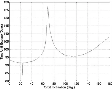
Figure 1.3: Time to escape for sail characteristic acceleration 0.75 mm/sec2_vs.

inclination, without shadow effects, (Ref.[8]).

variations through the centuries, this motion called planetary precession, due to attraction of the other solar system planets on Earth). Finally it is shown that the presence of shadow does not alter the optimal inclination. Here we report in Fig.1.3, taken from Ref.[8], which shows the times to escape, without shadow effects and from geostationary orbit (GEO), as function of initial orbit inclination. It can be noted the minimum time to escape for initial orbit lying onto the ecliptic plane, with sail achieving escape within the same plane.

1.4.6 The Dynamic Programming Algorithm: Some

Gen-eralities

The classic introductory material to Dynamic Programming (DP), its concept and applications can be find in books such as those by Bellman (1957), Bellman and Dreyfus (1962), Bertsekas (1995) Ref.[5], Bertsekas and Tsitsiklis (1996). Dynamic programming, has been introduced by Bellman (1957); it is a sequen-tial or multistage approach to formulating and solving mathematical program-ming problems. Reference [5] concerns about situations where decisions are made in stages; the outcome of each decision is not fully predictable, but can be anticipated to some extent, before the next decision is made. The objective is to minimize a certain cost, that is a mathematical expression of what is considered

(21)

an undesirable outcome.

A key aspect of such situations is that decisions cannot be viewed in isolation since one must balance the desire for low present cost with the undesirability of high future costs. The DP technique captures this traoff. At each stage, de-cisions are set based on the sum of the present cost and the expected future cost, assuming optimal decision making for subsequent stages. The DP algorithm is built upon the Bellman’s principle of optimality.

The problem types that can be solved by DP can be divided in:

• finite vs infinite state set • finite vs infinite horizon time • discrete vs continuous time • deterministic vs stochastic system.

We can already disclose that the time optimization for solar sail escape tra-jectories is an infinite state, finite horizon time, continuous time optimization problem for a deterministic (made the assumption that the state information is perfectly achievable) problem; for the application of DP in the performance index optimization the problem will be turned into one with finite state and discrete time.

Definitions and other generalities about the classical theory of DP will be formalized in Chapter 3. In the next section it will shortly follow a literature review concerning applications of DP in various aeronautical and astronautical optimal control problems.

1.4.7 Background on Dynamic Programming in Optimal

Control Problems for Aeronautical and

Astronauti-cal Applications

The early applications were carried out in 1968 by Nishimura and Pfeiffer, with the DP employed to solve the problem of the optimal stochastic orbit transfer strategy. This latter is defined as the sequence of guidance corrections which will minimize a statistical measure of final error, subject to the constraint that the total correction capability expended, be less than a specified number. This is an application example of DP to an imperfect state information problem. In such situations at each stage the controller receives some observations about the value of the current state which may be corrupted by stochastic uncertainty.

At that time storing capabilities of digital computers were limited and the so-called (by Bellman) ”curse of dimensionality”, was the biggest limitation using

(22)

DP algorithm. In fact, for high-dimensional systems the number of high-speed storage location becomes prohibitive. In the Nishimura’s study the numerical difficulty of storing the many values of the optimized performance index, corre-sponding to every discrete value of the state variables is overcome by neighbor-hood of local minima. The computer program designed to solve this problem is described, and some numerical results applicable to a space mission of a Voyager type have been presented.

More recently, in a work by Dohrmann, Eisler, and Robinett (1996), Ref.[18], a method has been presented for burnout-to-apogee munitions guidance that corrects launch offsets from a nominal, ground-to-ground trajectory. A guidance problem with an unspecified final time has been transformed to a form solvable by the method of dynamic programming.

In certain kind of problems DP provides a methodology for optimal deci-sion making under uncertainity, like in the Nishimura’s article. In a work by Chakravorty and Hyland (2000), Worst Case Dynamic Programming and Its

Application to Deterministic Systems, the numerical solution of discrete time,

infinite horizon, stationary DP problem has been investigated. Results are il-lustrated through an orbital dynamics example.

A study by Murray, Cox, (2000) and others, presented results of research NASA’s Hyper-X Program, in which an advanced controller, for the X-43LS vehicle, employed a modification to the ”Adaptive Critic methods”, that im-plement approximate Dynamic Programming for designing (near) optimal con-trollers for nonlinear plants.

In an article by Blin, Bonnans (2001) and others (Ref.[19]) the problem of identifying an optimal time to manoeuvre for an air traffic system, and the ma-noeuvre itself, has been formulated as a problem of optimal control of a dynamic system, and modeled by the Hamilton-Jacobi-Bellman equation (Chap. 3, Eq. (3.10)). The dynamic programming (DP) approach has been used to solve this equation for a dynamic system. The paper proposed an initial problem state-ment (including the HJB equation and a cost function), with a possible dynamic programming algorithm to solve it. The identification of the optimal time to manoeuvre and the manoeuvre itself have been formulated as minimizing a given cost, that is, a mathematical function which defines what is an undesirable out-come. In addition to the cost function, operational constraints have been also considered, and formulated as inequalities or domain definitions. The decision making is a step by step process, based on dynamic programming. This means that at each stage, decisions or controls, are based on both the current cost and on the future expected cost. This method ensures an optimal control of a

(23)

dynamic system over a finite number of stages (finite horizon time), as it has been outlined in this work.

Recent work by Bayen, Callantine (2004) and others (Ref.[20]), presented the application of DP to a combinatorial optimization problem to achieve proper ar-rival runway spacing, which appears in the process of assigning speed during the transition to approach, and approach phases of flight. A dynamic programming based algorithm computed the maximum minimum spacing between aircraft upon landing, and investigated the sensitivity of the spacing to perturbations.

To conclude, it appears that the problem of time optimization for solar sail escape trajectories has never been addressed using a DP approach.

(24)

Chapter 2

The Solar Sail Escape

Problem

2.1 Solar Sail Performances

Let us start with defining a parameter required in trajectory analysis of a sail-spacecraft, the characteristic acceleration S0, which is defined as the acceleration

that the spacecraft would experience at 1 astronomical unit (AU) distance from the Sun when the sail is oriented normal to sunlight. Under the hypothesis that solar radiation pressure has an inverse square variation with the distance from the Sun, the solar sail acceleration due to solar radiation pressure, when the sail is oriented normal to sunlight, is given by:

aR= S0/R2 (2.1)

with R expressed in AU .

The characteristic acceleration is usually expressed by the dimensionless sail

loading parameter β, defined to be the ratio of acceleration due to solar radiation

pressure, to solar gravitational acceleration due to the Sun in a given point of the space:

β , aR k agravk

(2.2) Since both solar radiation pressure acceleration and solar gravitational acceler-ation depend on the inverse square of distance from Sun, β is independent by the latter, thus we can even define β as:

β = σ

∗

(25)

where σ∗ _{is the critical solar sail loading parameter set to 1.53 g/m}2 _{which is}

function of the solar mass and solar intensity W (set to 1368 W/m2 _{at 1 AU),}

and

σ , m

A (2.4)

is the ratio of the sail mass to its surface, called sail loading.

The specific impulse for a rocket is related to propellant used, and can be expressed by:

Isp=

ve

g0

(2.5) where veindicates the exhaust propellant velocity relative to the rocket, and g0

is the gravity acceleration at sea level. Burnt propellant is related to specific impulse by the well-known Tsiolkovsky’s equation:

∆v = Ispg0ln(m1 m2

) (2.6)

that can be written as:

m1− m2

m1 = 1 − exp(−

∆v

Ispg0) (2.7)

where m1and m2are respectively initial and burnout mass (or mass at the end of

the thrust period), and ∆v is the velocity variation required by a given mission.

For a solar sail there is no fuel consumption, which means that m1= m2. Thus

from equation (2.7) we would get therefore an infinite specific impulse.

For obtaining anyway a specific impulse evaluation brought by a sail, to compare various solar sails, specific impulse can be defined again. Initial mass

m1 can be defined as structural and payload mass, while m2 as payload mass.

From equation (2.6) it even results:

m2

m1 = exp(−

∆v

g0Isp) (2.8)

thus for Ispwe get:

Isp= ∆v

g0ln(1/R) (2.9)

where R = m2/m1. For a mission whose duration is ∆t, the required ∆v can

be approximate by:

∆v = aR∆t (2.10)

where aRis given by (2.1). Hence Ispcan be expressed as proportional through

the following relation:

Isp∝ aR∆t

g0ln(1/R) (2.11)

Relation (2.11) shows how the Ispis directly proportional to the flight time and

(26)

Figure 2.1: Inertial X-Y-Z and Rotating Sun-Oriented α-β-Z Coordinate Sys-tems

competitive for long duration missions and when aR becomes bigger, that is,

close to the Sun.

2.2 Reference Frames

The coordinate systems used in the Coverstone and Prussing paper are main-tained (Ref. [7]). Some of the following figures, used to show reference frames, are taken from Ref. [6].

A two-body gravity model is used, with the gravitational effects of tertiary bodies, such as the Sun, neglected. The reference orbit plane is the ecliptic. Two coordinate systems will be used, as illustrated in Fig. 2.1. The XY Z axes are Sun centered inertial axes with the X axis directed to the first point in Aries. The α − β − Z axes are Earth centered with α − β in the ecliptic plane. These axes rotate with the apparent motion of the Sun, so that the α-axis is always oriented from the Earth to the Sun.

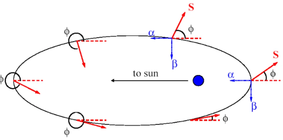
Sail orientation is defined by two control angles: the in-plane control angle,

φ, and out-of-plane control angle, θ. As can be seen from Fig. 2.3, φ is measured

counter-clockwise from the negative α-axis in the orbit plane. Figure 2.4 defines

θ as the angle measured from the ecliptic plane. Since we will study the

2-dimensional case, we can set

θ = 0

(27)

tra-Figure 2.2: In-plane Control Angle (on the ecliptic plane), φ, Definition

(28)

Figure 2.4: Out-of-plane Control Angle, θ, Definition jectories will lie therefore on the ecliptic plane.

2.3 Solar Radiation Pressure

Solar radiation pressure is adjusted according to the inverse square of the dis-tance from the sun, with reference to solar radiation pressure at 1 AU from the Sun, which is:

p1= 4.56 · 10−6 N · m−2

Hence the relation for the solar radiation pressure as function of the distance from the Sun will be:

p(r) = p1/r2 (2.12)

with r expressed in AU .

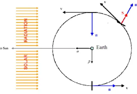
Solar radiation pressure is modeled as a constant vector field aligned with the α-axis since all distances considered in the escape are small relative to the distance from the Earth to the Sun. This detail is depicted in Fig. 2.5, in which the unit vector n represents the normal to the solar sail.

2.4 Equations of Motion

The equation of motion for a solar sail with respect to a geocentric inertial frame are:

˙r = v (2.13)

˙v = −µ⊕

r3 r + S (2.14)

where S is the acceleration due to the solar radiation pressure misured in the in-ertial frame, µ⊕ is the Earth’s gravitational parameter, and [r]T⊕ = [rx, ry, rz]T

and [v]T⊕ = [vx, vy, vz]

T _{are respectively the position and velocity vector in T} ⊕.

(29)

Figure 2.5: Solar Radiation Pressure, Sail Acceleration, and Sailcraft Velocity at Various Points in the Ecliptic Plane

2.5 Ideal Sail Acceleration Model and Two-Dimensional

Case

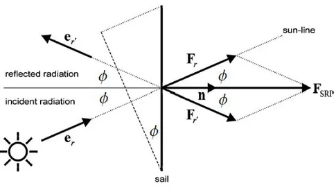
Concerning the ideal solar sail model, the following assumption is made: the sail is regarded as a flat perfect mirror so that we can neglect the diffused and absorbed light.

The acceleration on a flat ideal sail is given in Ref. [1] as:

S = (2W A/mc)(ˆn · ˆα)2_{n = S}_ˆ

0(ˆn · ˆα)2nˆ (2.15)

where W is the solar intensity at 1 AU from the Sun, A is the sail area, c is the speed of light in vacuum, ˆn is the unit vector normal to the sail, and ˆα is a unit

vector in the direction of the Sun. The squared term in Eq. (2.15) represents the variation in the sail acceleration according to the square of the cosine of the angle between the sail normal and the direction of the Sun. For the ideal sail assumed, the sail force is normal to the sail.

In the two-dimensional case both the normal to the sail and the sail acceler-ation will lie on the ecliptic plane. With regarding to Fig. 2.2, the unit vector normal to the sail in terms of components in the α − β − Z frame:

ˆ

(30)

Figure 2.6: Force on ideal solar sail due to specular reflection and the unit vector in the direction of the Sun:

ˆ

α = [1 0 0]T_. _(2.17)

The Eq. (2.15) becomes:

S(φ) = S0(− cos φ)2[− cos φ − sin φ 0]T (2.18)

which can be written as:

S(φ) = −S0     cos3_φ sin φ cos2_φ 0     (2.19) where φ ∈ [−π/2, π/2].

2.6 Position Vector in the αβZ Coordinate

Sys-tem

To write the position vector in the α − β − Z coordinate system, we use the frame ˆP ˆQ ˆW (perifocal system) and shown in Fig. 2.7, in which ˆP is the unit

vector pointing from the focus to the perigee; ˆQ is a unit vector normal to ˆP

and belonging to the orbital plane in a way that ˆ

(31)

Figure 2.7: Orientation of the orbit, through the ² angle, in the α − β − Z frame results in the same wise of the specific angular momentum of motion:

h = r × v

. We make the assumption that this frame is inertial for small orbit changes during a period. The ε angle, positive in counter clock-wise from the positive direction of the α axis, defines the orbit orientation in the α − β − Z frame, as shown in Fig. 2.7. In ˆP ˆQ ˆW , the expression of r is given:

r = r(cos νP + sin νQ) (2.20) where r = h 2_/µ ⊕ 1 + e cos ν,

and ν is the true anomaly. From the definition of eccentricity vector we have:

² = arctaneβ eα

(2.21) By looking at Fig. 2.7 the position vector expression in the α−β −Z coordinate system is given by:

[r]αβZ = r[cos(ε + ν) sin(ε + ν) 0]T (2.22)

2.7 Circular Orbits

For circular orbits, the position is usually defined through the true longitude l: cos lα · rˆ

(32)

hence measured counter-clockwise starting from the positive α direction. Since we are concerned with escape trajectories, even starting from an elliptic orbit, a circular one could appear during escape. Therefore we will consider circular the orbits, such that e < 10−4_{. To guarantee continuity in perigee orientation we}

can assume as frozen the perigee at time when eccentricity drops under 10−4_,

and restart the variation of the perigee orientation when eccentricity overcomes the above-mentioned value.

(33)

Chapter 3

Optimal Control:

Dynamic Programming

The application of optimal control lies on searching the time history of control that minimizes or maximizes a given function. In this study a method called Dynamic Programming (DP) has been used; it has been developed by R. E. Bellman (1957), (Ref. [3], [4], [5]). In this chapter we will delineate some generalities about the classical theory of DP and see that it leads to a recurrence equation that is amenable to solution by use of digital computers. Hereafter we will also assume that the state is perfectly known at each stage, that is the problem is deterministic.

3.1 The Extremal Field Approach

Let us consider the general control problem for a system whose state equations are

˙x = f (x(t), u(t), t) with x(t0) = x0 (3.1)

where x(t) ∈ <n_{defines the system state and u(t) ∈ <}m_{defines the control. Let}

us suppose that we want to find the optimal control functions u∗_{(t), that is, the}

control functions that minimizes a given function, from a great many different initial points to a given terminal hypersurface in the space state defined by the terminal constraint

ψ[x(tf), tf] = 0. (3.2)

where tf is the final time, and x(tf) is the system state at the final time. To

(34)

the possible initial points are on, or at least very close to, one of our calculated optimal paths. In the literature of the calculus of variation, such a family is called a field of extremals. In general, only one optimal path to the terminal hypersurface will pass through a given point (x(t), t), and a unique optimal

control vector u∗_{(t) is then associated with each point. Hence we may write}

u∗_{= u}∗_{(x, t).} _(3.3)

This is the optimal feedback control law. The control vector is given as a function of the present state x(t) and the present time t. Associated with starting from a point (x, t) and proceeding optimally to the terminal hypersurface, there is a

unique optimal value of the performance index, J∗_{. We may therefore regard}

J∗ _{as a function of the initial point, that is,}

J∗_{= J}∗_{(x, t).} _(3.4)

This is the optimal return function (or performance index or cost function).

3.2 Dynamic Programming

One aspect of the classical Hamilton-Jacobi theory (Ref. [3]) is concerned with finding the partial differential equation satisfied by the optimal return function

J∗_{(x, t). There is also a partial differential equation satisfied by the optimal}

control function u∗_{(x, t). Bellman has generalized the Hamilton-Jacobi theory}

to include multistage systems and combinatorial problems and he called this overall theory dynamic programming.

3.2.1 The Partial Differential Equation for the Optimal

Return Function

Let us consider again the general control problem for a system whose state equations are given by (3.1) with terminal boundary conditions

ψ[x(tf), tf] = 0. (3.5)

The performance index can be expressed by:

J = ϕ[x(tf), tf] +

Z tf

t

L[x(τ ), u(τ ), τ ] dτ (3.6) where ϕ and L are specified functions, tfis fixed, t can be any value less than or

(35)

of integration; the optimal performance index is given by: J∗_{(x, t) = min} u(t){ϕ[x(tf), tf] + Z tf t L[x(τ ), u(τ ), τ ] dτ } (3.7) with the boundary condition at t = tf:

J∗(x, t) = ϕ(x, t) on the hypersurface ψ(x, t) = 0 (3.8)

We define the Hamiltonian H function as:

H(x(t), u(t),∂J∗

∂x, t) , L[x(t), u(t), t] + ∂J∗

∂x(x(t), t) · f (x(t), u(t), t) (3.9)

and as it can be found in Ref.[3], it finally results:

−∂J ∗ ∂t = H ∗_(x,∂J∗ ∂x, t) (3.10) where H∗(x,∂J ∗ ∂x, t) = minu∈UH(x, ∂J∗ ∂x, u, t). (3.11)

and U is the domain of feasible control. Equation (3.10) is called the

Hamilton-Jacobi-Bellman Equation(H-J-B); it is a first-order nonlinear partial differential

equation and it must be solved with the boundary condition (3.8).

Equation (3.11) states that u∗ _{is the value of u that minimizes globally the}

Hamiltonian H(x, ∂J∗_{/∂x, u, t), holding x, ∂J}∗_{/∂x, and t constant; this is}

an-other statement of the Minimum Principle. The H-J-B equation represent a necessary and sufficient condition for optimality; in fact, the minimum cost function J∗_{(x(t), t) must satisfy the H-J-B equation for optimality (necessity).}

It can also be given proof that if there is a cost function J0_{(x(t), t) that satisfies}

the H-J-B equation, then J0 _{is the minimum cost function (sufficient condition).}

3.2.2 Discrete Approximation

Only rarely it is feasible to solve the Hamilton-Jacobi-Bellman partial differen-tial equation for a nonlinear system of any practical significance, and, hence, the development of exact explicit feedback guidance and control schemes for nonlinear systems is usually out of reach.

In this section we will show that DP leads to a functional recurrence relation when a continuous process is approximated by a discrete system. The

princi-ple of optimality is the cornerstone upon which the computational algorithm is

(36)

Figure 3.1: Optimal path from a to e

3.3 The Principle of Optimality

Using DP, an optimal policy is found by employing the concept called principle

of optimality whose name is due to Bellman. The optimal path for a multistage

decision process is shown in Fig. 3.1.

Suppose that the first decision (made at a) results in segment a-b with cost

Jaband the remaining decisions yield segment b-e at a cost of Jbe. The minimum

cost J∗

ae from a to e is therefore

Jae∗ = Jab+ Jbe (3.12)

Assertion: 3.3.1 If a-b-e is the optimal path from a to e, then b-e is the

optimal path from b to e.

The proof is given by contradiction and can be found in Ref. [4]. Bellman has called the above property of an optimal policy the principle of optimality:

An optimal policy has the property that whatever the initial state and the initial decision are, the remaining decisions must constitute an optimal policy with regard to the state resulting from the first decision.

3.3.1 Application of the Principle of Optimality to

Deci-sion Making

We briefly illustrate the procedure for making a single optimal decision with the aid of the principle of optimality. Consider a process whose current state is b. The paths resulting from all allowable decisions at b are shown in Fig.3.2(a). The optimal paths from c, d, and e to the terminal point f are shown in Fig.3.2(b). The principle of optimality implies that if b-c is the initial segment of the optimal path from b to f then c-f is the terminal segment of this optimal path. The same reasoning applied to the initial segments b-d and b-e indicates that the paths in

(37)

Figure 3.2: (a) Paths resulting from all allowable decisions at b. (b) Optimal paths from c, d, e to f . (c) Candidates for optimal paths from b to f .

Fig.3.2(c) are the only candidates for the optimal trajectory from b to f. The optimal trajectory that starts at b is found by comparing:

Cbcf∗ = Jbc+ Jcf∗

C∗

bdf = Jbd+ Jdf∗

C∗

bef = Jbe+ Jef∗

The minimum of these costs must be the one associated with the optimal deci-sion at point b.

Dynamic programming is a computational technique which extends the above decision-making concept to sequences of decisions which together define an op-timal policy and trajectory.

3.4 The Dynamic Programming Algorithm

Let us summarize the DP computational procedure for determining optimal policies. An n-th order time-invariant system is described by the state equation

˙x(t) = f (x(t), u(t)). (3.13)

The time invariance (t does not appear explicitly in f ) is assumed only to simplify the notation. The algorithm is easily modified if this is not the case

(38)

(Ref.[4]). It is desired to determine the control law that minimizes the perfor-mance measure: J = ϕ[x(tf)] + Z _t_f 0 L[x(τ ), u(τ )] dτ (3.14) where tf is assumed fixed. The admissible controls are constrained to lie in a set

U: u ∈ U. We first approximate the continuously operating system by a discrete

system; this is accomplished by considering N equally spaced time increments ∆t in the interval 0 ≤ t ≤ tf, and approximating the system differential equation

by a difference equation, and the integral in the performance measure must be approximated by a summation. Therefore we obtain:

x(t + ∆t) − x(t)

∆t ≈ f (x(t), u(t)) (3.15)

or

x(t + ∆t) = x(t) + f (x(t), u(t))∆t. (3.16) It will be assumed that ∆t is small enough so that the control signal can be approximated by a piecewise-constant function that changes only at the instants

t = 0, ∆t, ..., (N − 1)∆t; thus for t = k∆t:

x([k + 1]∆t) = x(k∆t) + f (x(k∆t), u(k∆t))∆t; (3.17)

k = 0, 1, ..., N − 1.

x(k∆t) is referred to as the k-th value of x and can be denoted by x(k). Thus

we can write:

x(k + 1) = x(k) + f (x(k), u(k))∆t, (3.18) which will be denoted by:

x(k + 1) , fD(x(k), u(k)). (3.19)

Operating on the performance index in a similar manner, we obtain:

J = ϕ(x(N ∆t)) + Z _∆t 0 L dt + Z _2∆t ∆t L dt + ... + Z _{N ∆t} (N −1)∆t L dt (3.20)

which becomes for small ∆t:

J ≈ ϕ(x(N )) + ∆t

N −1_X k=0

L(x(k), u(k)). (3.21)

which we will denote through:

J = ϕ(x(N )) +

N −1_X k=0

LD(x(k), u(k)). (3.22)

(39)

For every initial state x0, the optimal cost J∗(x0) is equal to J0(x0),

where the function J0 is given by the last step of the following

algo-rithm, which proceeds backward in time from period N −1 to period 0:

J∗

N −K(x(N − K)) = _{u(N −K)}min {LD(x(N − K), u(N − K)

+ J∗

N −(K−1)(fD(x(N − K), u(N − K)))} (3.23)

K = 1, 2, ..., N

with initial value

JN∗(x(N )) = ϕ(x(N )). (3.24)

The solution of this recurrence equation is an optimal control law u∗_{(x(N −}

K), N −K), K = 0, 1, ...N , which is obtained by trying all admissible control

values at each admissible state value.

To make the computational procedure feasible, it is necessary to quantize the admissible state and control values into a finite number of levels (grid).

3.5 Deterministic Finite States Systems and

Short-est Path

Following Ref.[5], in a deterministic problem where the state space Skis a finite

set for each k, then at any state xk, a control uk can be associated with a

transition from the state xk to the state xk+1of the form:

xk+1= f (xk, uk)

at a cost gk(xk, uk) of the corresponding transition. Thus a finite-state

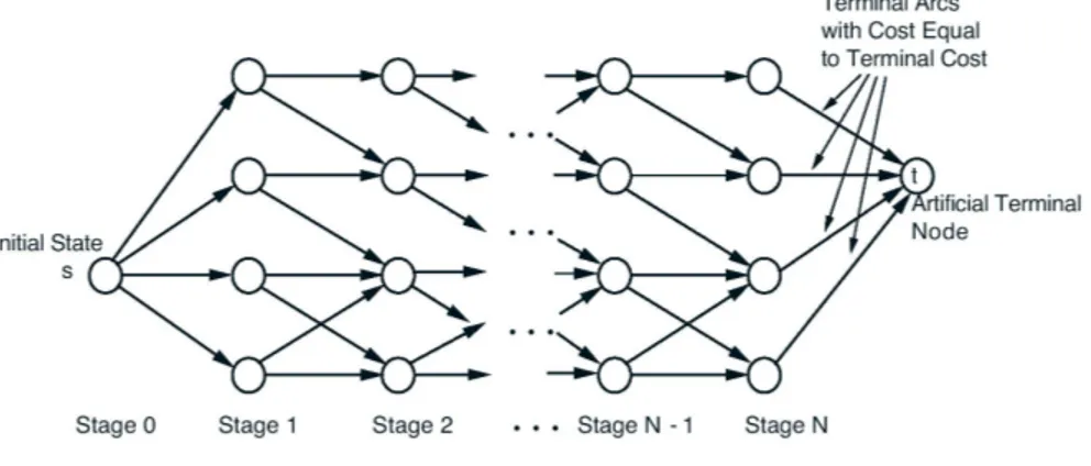
deter-ministic problem can be equivalently represented by a graph such as the one of Fig.3.3, where nodes corresponds to states, the arcs correspond to transitions between states at successive stages and each arc has a cost associated with it. To handle the final stage, an artificial final node t has been also added. Each

state xN at stage N is connected to the terminal node t with an arc having cost

gN(xN). Control sequences correspond to paths originating at the initial state

and terminating at one of the nodes corresponding to the final stage N . The cost of an arc can be viewed as its length, therefore a deterministic finite-state problem is equivalent to finding a minimum length (or shortest) path from the

(40)

Figure 3.3: Transition graph for a finite-state system

initial node s of the the graph to the terminal node t. By path is meant a se-quence of arcs of the form (j1, j2), (j2, j3), ..., (jk−1, jk), and by length of a path,

the sum of the length of its arcs. Let us denote:

ak

ij = Cost of transition at time k from state i ∈ Sk to state j ∈ Sk+1,

aN

it = Terminal cost of state i ∈ SN [which is gN(i)],

where it is adopted the convention ak

ij = ∞ if there is no control that moves the

state form i to j at time k. The DP algorithm takes the form:

JN(i) = aNit, i ∈ SN, (3.25)

Jk∗(i) = min_j∈S

k+1

[akij+ Jk+1(j)], i ∈ Sk, k = 0, 1, ..., N − 1. (3.26)

The optimal cost is J∗

0(s) and is equal to the length of the shortest path from

s to t.

3.6 Characteristics of DP solution

Let us summarize the characteristics of the computational procedure and the solution it provides.

Absolute minimum: Since a direct search is used to solve the functional recurrence equation (3.23), the solution obtained is the absolute minimum. DP makes the direct search feasible because instead of searching among the set of all admissible controls that cause admissible trajectories, we consider only those controls that satisfy an additional necessary condition, the principle of optimality.

(41)

Form of the optimal control: DP yields the optimal control in closed-loop or feedback form for every state value in the admissible region we know what is

the optimal control. However, although u∗_{is obtained in the form}

u∗(t) = f (x(t), t), (3.27)

unfortunately the computational procedure does not yield a nice analytical ex-pression for f . It may be possible to approximate f in some way, but if this cannot be done, the optimal control law must be implemented by extracting the control values from a storage device that contains the solution of Eq. (3.23) in tabular form.

High-dimensional system: For high-dimensional systems the number of high-speed storage location becomes prohibitive. This is the biggest limitation using DP algorithm. Bellman called this difficulty the ”curse of dimensionality”. There are, however, techniques that have been developed to alleviate this issue and can be found in specialized literature.

(42)

Chapter 4

Variation of Parameters

The object of this part of the study is the definition of the variation of the sail spacecraft state over discrete time intervals through state equations in dis-cretized form. Some simplifying assumptions must be made. First, the magni-tude of S0(1 mm/sec2) is quite small, resulting in a very small net change in

energy over anyone orbit. Hence, as consequence, orbital parameters variations are small on temporal intervals appropriately selected. Therefore, it is assumed that the state components variations are only functions of the orbital elements at t=0 (perigee); in other words, it is assumed that the sail force does no real work over one orbit. Similarly, the α direction is assumed to be constant over one orbit period.

4.1 Definition of System State, States Domain

and State Equation

We define the state of the system through the components of the eccentricity vector e, and the angular momentum of motion vector h of the osculating Ke-plerian orbit, in the geocentric rotating α − β − Z frame. Concerning with two-dimensional escape trajectories, lying onto the ecliptic plane, the only com-ponents not identically equal to zero, will be eα, eβ, hz; the control will be the

φ angle. It could be chosen other combinations of orbital elements to define the

state (for instance the semimajor axis a, the eccentricity e and the longitude of perigee ω), but this set of orbital elements appear to be more suitable to afterwards investigate the state space through a performance index. Therefore

(43)

the system state has been defined through: [x]_αβZ=     eα eβ hz     (4.1)

with x ∈ S ⊂ R3 _{where with S has been indicated the state space. For circular}

orbits we assume: [x]circ_αβZ=     0 0 hz     (4.2) and

The system is intrinsically time invariant. With the state definition (4.1), the Earth escape problem will be still time invariant since the direction of solar radiation is fixed with respect to the α, β, Z frame; thus state variation and performance index will not depend explicitly by time but only state and control dependence will result. Recalling the discretized state equation:

x(k + 1) = x(k) + f [x(k), u(k)]∆t, (4.3) the variations, for the discretized state augmentation, will be defined by:

    ∆eα ∆eβ ∆hz     =     eα(k + 1) − eα(k) eβ(k + 1) − eβ(k) hz(k + 1) − hz(k)     = f (eα(k), eβ(k), hz(k), φ(k))∆t (4.4)

where ∆t = T will be set, being T the period of the osculating Keplerian orbit, which is given when the state system is known. For osculating Keplerian orbit we mean the Keplerian orbit (orbit that the sailcraft would go along, if the acceleration due to solar radiation pressure was set at zero, obtaining a simple two-body problem) which corresponds to the state of the sailcraft at a given time instant. Equation (4.4) defines the variations over one orbit period T of the components of the e and h vectors as a function of these same components at the perigee. To find analytical expressions for the (4.4), equations of the variation of parameter method, this latter described in Ref. [2], will be analytically integrated over one orbit period. The analytical integrals will be calculated keeping the control angle φ constant over one orbit. This will mean to get a piecewise function for φ control, as described in Section 3.4.

The chosen domain contained in the state space is cylindrical and has been

taken: _q

e2

Optimization of Ideal Solar Sails Earth Escape Trajectories using Dynamic Programming

Abstract

Acknowledgements

Ringraziamenti

Table of Contents

Chapter 1

Introduction

1.1

Motivation

1.2

Objectives

1.3

Models and Hypothesis used in the Work

1.4

Literature Review

1.4.1

The Solar Sail Concept through the XX

Century

1.4.2

Solar Sail Physical Models

1.4.3

Background on Solar Sails Trajectories

Optimiza-tion

1.4.4

The MIRITOE Control Law

1.4.5

Optimal Inclination for Planet-Centered Solar

Sail-ing

1.4.6

The Dynamic Programming Algorithm: Some

Gen-eralities

1.4.7

Background on Dynamic Programming in Optimal

Control Problems for Aeronautical and

Astronauti-cal Applications

Chapter 2

The Solar Sail Escape

Problem

2.1

Solar Sail Performances

2.2

Reference Frames

2.3

Solar Radiation Pressure

2.4

Equations of Motion

2.5

Ideal Sail Acceleration Model and Two-Dimensional

Case

2.6

Position Vector in the αβZ Coordinate

Sys-tem

2.7

Circular Orbits

Chapter 3

Optimal Control:

Dynamic Programming

3.1

The Extremal Field Approach

3.2

Dynamic Programming

3.2.1

The Partial Differential Equation for the Optimal

Return Function

3.2.2

Discrete Approximation

3.3

The Principle of Optimality

3.3.1

Application of the Principle of Optimality to

Deci-sion Making

3.4

The Dynamic Programming Algorithm

3.5

Deterministic Finite States Systems and

Short-est Path

3.6

Characteristics of DP solution

Chapter 4

Variation of Parameters

_Century