ALMA MATER STUDIORUM - UNIVERSITA' DI BOLOGNA
SCUOLA DI INGEGNERIA E ARCHITETTURA DIPARTIMENTO DI INGEGNERIA INDUSTRIALE
CORSO DI LAUREA MAGISTRALE IN INGEGNERIA ENERGETICA
TESI DI LAUREA in
ENERGETICA DEGLI EDIFICI E IMPIANTI TERMOTECNICI M
MODELLING OF DECENTRAL DHW PREPARATION IN LARGE
MULTI-FAMILY BUILDINGS
CANDIDATO RELATORE
Stefano Fisco Chiar.mo Prof. Ing. Gian Luca Morini
CORRELATORI Dr.-Ing. Fabian Ochs Dr.-Ing. Georgios Dermentzis
Anno Accademico [2018/2019] Sessione [I]
iii
Contents
Chapter 1. Introduction ... 13
1.1. Motivation of the work ... 13
1.2. Overview of the project ... 15
Chapter 2. Methodology ... 17
2.1. Boundaries of the project ... 17
2.2. Dynamic simulation tool. ... 18
2.3. Simulation models ... 19
2.3.1. DHW preparation model, flat-level ... 19
2.3.2. DHW preparation model, building-level ... 20
2.4. Controllers ... 22
2.4.1. Storage charging-pump controller ... 22
2.4.2. Mixer-diverter controller ... 23
2.4.3. Storage discharging-pump controller ... 25
2.4.4. User mass flow controller ... 25
2.5. DHW profiles ... 27 2.5.1. Standard EN16147 ... 27 2.5.2. Stochastic profile ... 29 2.5.3. Simultaneity factor ... 29 2.5.4. Implemented DHW profiles ... 30 2.5.4.1. Flat-level ... 30 2.5.4.2. Building-level ... 32
2.6. Parametrization of the models ... 36
2.6.1. Flat-level model ... 36
2.6.2. Building-level model ... 39
iv
3.1. Results of the flat-level model ... 44
3.1.1. Energy evaluation ... 45 3.1.2. Comfort ... 46 Temperature development ... 46 Dynamic behaviour ... 54 3.1.3. Discussion ... 56 3.2. Building-level results ... 57 3.2.1. Energy evaluation ... 57 3.2.2. Comfort ... 59 Temperature development ... 59 Dynamic behaviour ... 65
Chapter 4. Comparison between one HX per flat and one HX for the whole building ... 67
4.1. Concept ... 67
4.2. Simulation model and DHW profiles ... 69
4.3. Comparison results ... 69
Chapter 5. Conclusions ... 71
Acknowledgment ... 74
vi
List of symbols and abbreviations
CHX Thermal capacity of the heat exchanger [J/K] cp Specific heat [J/kgK]
DHHX District heating heat exchanger DHW Domestic hot water
E Energy [J]
fdiv Control signal of the mixer-diverter FE Final Energy
fs Smultaneity factor FWS Fresh water station HP Heat pump
HP Heat pump HX Heat exchanger
iPHA International passive haus association m Mass [kg]
ṁ Mass flow [kg/s]
PHPP Passive House Planning Package Q Energy [J]
s Thickness [mm] S Surface [m2]
Tbot Bottom temperature of the storage [°C] Ttop Top temperature of the storage [°C] UAHL Heat transfer coefficient to ambient [W/K]
UAHX Heat transfer coefficient between primary and secondary side heat exchanger [W/K] UE Useful energy V Volume [m3] Δθ Temperature difference [K] θ Temperature [°C] λ Termal conductivity [W/(m·K)] ρ Density [kg/m3]
vii
Extended abstract
This master thesis contributes to the need to design more efficient heating and domestic hot water preparation systems to support the ambitious need of limiting the CO2 emissions in accordance to the European goals. While for heating good solutions were developed within the last decades, there is still a need for improving domestic hot water (DHW) preparation and supply systems, which represent, nowadays, a considerable percentage of the total energy expense in households, especially in good energy performance buildings such as Passive Houses.
In this context, dynamic building and simulation plays an important role in the development of DHW preparation systems for residential buildings, in order to evaluate and optimize the final energy and the DHW comfort (evaluated as temperature of the DHW supplied to the user and the so-called “waiting time” to reach the set point of this temperature).
The case study of this work is a big multi-family building composed of 96 flats that will be built in the neighbourhood “Campagne” in Innsbruck.
A fresh water station (FWS) is placed in each flat for the DHW preparation. FWS is a unit for the decentral, i.e. flat-wise instant DHW preparation, and it is composed by one heat exchanger (HX), and the control systems implemented in order to respond to the user requests and assure the working conditions of the HX. In this specific case study, district heating (DH) is used to heat up the water in the storage tank located in the technical room of the building. A distribution system connects the storage to all the FWS in the flats.
Energy and comfort evaluations are strongly influenced by the DHW profiles. For the flat-level simulations, these profiles can be either derived from standard profiles, e.g. EN16147 (here, profile M) or from stochastic tools, e.g. such as DHWcalc, which creates a DHW profile using a stochastic approach (flat-level and building level DHW profiles).
The physical approach for the simulation of DHW preparation on building-level is to simulate the whole building with one HX in each flat: for big multi-family buildings, this approach would lead to a very heavy model and extensive simulation times. The second approach is to simulate the DHW preparation on flat-level and then extrapolate the results to the whole building: however, this method significantly overestimates the required heating power. The third approach is to simulate the building-level DHW preparation with a single HX which approximates the behaviour of all the HXs of the building. For this purpose, the simultaneity factor (fs) should be considered (i.e the simultaneity of DHW use). For the building-level DHW
viii
preparation, in fact, it is important to consider that only a limited number of flats will consume the DHW at the same time and so that the building peak loads cannot be evaluated as the sum of the peak loads of each flat. In the framework of this thesis, the third approach is chosen as the most appropriate for the simulations. However, in order to prove the reliability of the approach, this approach is compared to the physical approach, using a small multi-family building composed of 10 flats.
In order to parametrize the HX for the whole building, a DHW profile for the building should be derived (building-level DHW profile). The DHW profile for a building is implemented through the generalization of the profiles derived for the flat. Four different DHW profiles for the building are implemented: 1) hourly average profile (i.e. the tappings derived from standard EN16147, profile M, averaged to hourly time steps); 2) 10 seconds profile (i.e. a profile derived from EN16147 where the daily tapping cycle of each flat occurs with a delay of 10 seconds for each flat); 3) 39 seconds profile (same profile as the second one but with a delay of 39 seconds for each flat); 4) stochastic profile (i.e. a profile derived from DHWcalc which distributes the daily tapping all over one day, setting reference conditions such as volume of DHW daily required and duration of the tappings).
First, a representative model of the FWS for each flat is implemented in Matlab/Simulink simulation environment, considering a 35 kW HX (which corresponds to a HX of a typical market available FWS). The two flat-level profiles are tested on this model together with two different control strategies of the circulation pump, showing that the control strategy influences how the set point temperature of the DHW supplied to the user is achieved (useful energy and waiting time).
From the flat-level model, a building-level model is derived. The four different building-level profiles are used to evaluate the simultaneity factor, and so the peak load of the building, in order to size the HX for the whole building. For each profile three main parameters of the heat exchanger are calculated: heat transfer coefficient between primary and secondary side (UAHX), heat transfer coefficient to the ambient (UAHL) and thermal capacity (CHX).
The DHW profiles (and so the simultaneity factor fs) and the parametrization of the HX influence the results. Final energy and DHW comfort (i.e. the DHW temperature and the “waiting time” to reach this temperature) are compared in each case. The return temperature of the fluid sent back to the storage is also analysed. The development of the return temperature to the storage is influenced by the DHW profiles and the thermal capacity of the pipe. The return temperature to the storage has similar developments for all the analysed DHW profiles,
ix
except for the 10s profile which is the one with the highest fs. With this profile, the return temperature to the storage is higher in the period between 13:00 and 22:00. For this reason, the thermal losses observed with the 10s profile are higher if compared to the other cases.
In future works the influence of the insulation of the pipe on the return temperature to the storage (and so on the thermal losses) should be evaluated. Future studies should also investigate the influence on the results of different boundary conditions and DHW system design.
x
Extended abstract
Il lavoro svolto contestualmente a questa tesi risponde all’esigenza di progettare efficienti sistemi di riscaldamento e produzione di acqua calda sanitaria (ACS), seguendo gli ambiziosi obiettivi europei in materia di riduzione delle emissioni di CO2. Per i sistemi di riscaldamento sono state sviluppate ottime soluzioni nell’arco degli ultimi anni, ma importanti sforzi sono ancora da compiere per ottimizzare i sistemi di produzione e distribuzione di ACS che rappresentano, ad oggi, una percentuale considerevole della spesa energetica nelle abitazioni (specialmente in edifici con buone prestazioni energetiche, come le Passive Houses).
In questo contesto, la simulazione dinamica degli edifici gioca un ruolo fondamentale nello sviluppo di sistemi di produzione di ACS per edifici residenziali, permettendo di valutare ed ottimizzare il consumo di energia e il comfort (valutato rispetto alla temperatura dell’ACS fornita all’utente e il cosiddetto “waiting time”, ovvero il tempo necessario per il raggiungimento del set point di questa temperatura).
Il caso studio di questo lavoro è un grande edificio multi-familiare, composto da 96 appartamenti, che verrà costruito nel quartiere “Campagne”, nella città di Innsbruck.
Una fresh water station (FWS) è collocata in ciascun appartamento ed è utilizzata per la produzione di ACS. Una FWS è un’unità decentrata per la produzione istantanea di ACS nell’appartamento, ed è composta da uno scambiatore di calore (HX) e dai sistemi di controllo che permettono di rispondere prontamente alle richiese dell’utenza, assicurando le condizioni di funzionamento dell’HX. In questo specifico caso studio, la connessione ad una rete di teleriscaldamento (DH) è utilizzata per riscaldare l’acqua presente all’interno di un serbatoio di stoccaggio termico, posizionato nel locale tecnico dell’edificio. Un sistema di distribuzione collega il serbatoio a tutte le FWS negli appartamenti.
Le valutazioni energetiche e sul comfort sono fortemente influenzate dai profili d’uso dell’utenza (DHW profiles). Per la simulazione di un unico appartamento (flat-level), il profilo d’uso può essere ricavato da un profilo standard, ad esempio EN16147 (profilo M, nel caso di questo lavoro) o da appositi tools, ad esempio DHWcalc, che permette di creare un profilo d’uso seguendo un approccio stocastico.
L’approccio fisico per simulare la produzione di ACS per l’intero edificio (building-level), prevede la simulazione dell’intero edificio con un HX in ciascuno degli appartamenti: per grandi edifici multi familiari, questo approccio richiederebbe l’implementazione di un modello troppo pesante, nonché tempi di simulazione eccessivi. Il secondo approccio simula la
xi
produzione di ACS per un singolo appartamento, per poi estrapolare i risultati all’intero edificio: questo metodo tende a sovrastimare la potenza richiesta per la produzione dell’ACS. Il terzo approccio simula la produzione di ACS per l’intero edificio, tramite un singolo HX che approssima il comportamento di tutti gli HXs dell’edificio. Per poter dimensionare questo HX, è necessario tenere in considerazione l’effetto del simultaneity factor fs (ovvero il fattore di simultaneità dell’uso di ACS nell’edificio). Per la produzione di ACS per l’intero edificio, infatti, è importante considerare che solo un limitato numero di appartamenti richiederà ACS nello stesso momento e quindi il carico di picco dell’edificio non può essere valutato come la somma dei carichi di picco di ciascun appartamento. Nell’ambito di questa tesi, è stato scelto il terzo approccio come il più appropriato per le simulazioni. Tuttavia, per esaminare l’affidabilità di questo approccio, lo stesso è stato confrontato con l’approccio fisico, usando un edificio multi familiare più piccolo, composto da 10 appartamenti.
Al fine di parametrizzare l’HX per l’intero edificio, è necessario ricavare un profilo d’uso di ACS dell’intero edificio. Il profilo d’uso di ACS per l’intero edificio è implementato attraverso la generalizzazione dei profili d’uso ricavati per un appartamento. Sono stati implementati quattro diversi profili d’uso di ACS dell’edifico: 1) profilo orario medio (i.e. i prelievi d’acqua ricavati dal profilo standard EN16147, sono stati mediati su un time step di un’ora); 2) profilo ogni 10 secondi (i.e. un profilo derivato da EN16146 in cui il ciclo giornaliero di prelievi d’acqua per ciascun appartamento inizia con un ritardo di 10 secondi); 3) profilo ogni 39 secondi (stesso profilo del secondo caso ma con un ritardo di 39 secondi per ciascun appartamento); 4) profilo stocastico (i.e. un profilo derivato dal DHWcalc che distribuisce i prelievi giornalieri lungo l’arco di una giornata, sulla base di input come il volume di ACS richiesto in un giorno e la durata dei prelievi di ACS).
Per primo è stato sviluppato e dimensionato un modello rappresentativo della FWS di ciascun appartamento, nell’ambiente di simulazione Matlab/Simulink, considerando un HX di 35 KW (corrispondente alla taglia di un HX di una tipica FWS disponibile in commercio). Su questo modello sono stati testati i due diversi profili d’uso di un appartamento e due diverse strategie di controllo della pompa di circolazione, mostrando le modalità con cui la strategia di controllo influenza il raggiungimento della temperatura di set point dell’ACS fornita all’utenza (energia utile e waiting time).
Dal modello della FWS dell’appartamento è stato ricavato un modello di FWS per l’intero edificio. I quattro diversi profili d’uso dell’edifico sono utilizzati per valutare il simultaneity factor, e quindi il carico di picco, in modo da poter dimensionare l’HX per l’intero edificio. Per
xii
ciascun profilo sono stati calcolati tre diversi parametri dell’HX: coefficiente di scambio termico tra il circuito primario e secondario (UAHX), coefficiente di scambio termico con l’ambiente (UAHL) e capacità termica (CHX).
Il profilo d’uso di ACS (e quindi il simultaneity factor) e la parametrizzazione dell’HX influenzano i risultati. L’energia per la produzione di ACS e il comfort termico (i.e. temperatura dell’ACS e “waiting time” per raggiungere questa temperatura) sono confrontati nei diversi casi. Anche l’andamento della temperatura di ritorno dell’acqua al serbatoio di stoccaggio termico è analizzata. L’andamento di questa temperatura è influenzato dal profilo d’uso di ACS e dalla capacità termica dei tubi. La temperatura di ritorno al serbatoio di stoccaggio termico ha un andamento simile per ciascuno dei casi analizzati con i diversi profili d’uso, tranne che per il caso denominato profilo ogni 10 secondi, che è il profilo con il più alto valore del simultanety factor. Nel periodo tra le 13:00 e le 22:00, infatti, con questo profilo d’uso, si osserva che il valore della temperatura di ritorno al serbatoio è più alto rispetto agli altri casi.
In sviluppi futuri dello studio, verrà valutata l’influenza dell’isolamento termico sulla temperatura di ritorno al serbatoio termico. Studi futuri, inoltre, indagheranno l’influenza sui risultati di diverse condizioni al contorno e di diversi design del sistema di produzione di ACS.
13
Chapter 1. Introduction
1.1.
Motivation of the work
Residential buildings are known to strongly influence energy consumption. In developed countries, up to 40% of total energy consumption is spent in residential sector, exceeding industrial and transportation sectors (Perez-Lombard, Ortiz, & Pout, 2007). Deep studies on how to reduce this expense are always in the spotlight in the scientific field.
Many of the studies found in literature are focused on how to improve simulation studies in order to optimize energy consumption of the buildings (Dermentzis, et al., 2017); (Dermentzis, et al., 2019). These studies, focused on dynamic simulation methods, aim to reduce the amount of energy consumption imputable to heating systems.
The energy consumption for DHW (Domestic Hot Water) preparation still remains a not-deeply studied topic in dynamic simulation. DHW usage per person can be 30% higher than the values assumed in planning tool like PHPP (Clarke & Grant, 2010).
A residential district will be built in Innsbruck (Austria) and its energetic optimization is the core of the so-called Campagne research project, which aims to minimize the environmental impact of a multi-family building district. Previous studies have already compared different heating generation systems (Dermentzis, 2019). The aim of this work, instead, is to deeply investigate the modelling DHW preparation for big multi-family buildings, excluding space heating. The considered reference building is a 96-flat building.
A model for DHW preparation is implemented for a single flat (flat-level DHW preparation). In order to simulate the DHW preparation for the whole building, this model can be used for each of the flats. This approach is used for small multi-family building (10-flat building). However, for a big multi-family building it would be hard to implement and it would be time and computational consuming. Thus, an alternative method to simulate the DHW preparation for the whole building (building-level DHW preparation) is developed with a central HX that covers the request of the whole building.
In the proposed method, the parametrization of the HX is crucial. The parameters of the HX are assumed in order to approximate the behaviour of all the HXs of the building together.
The length and the diameter of the pipes strongly influences the heat losses (van der Heijde, Aertgeerts, & Helsen, 2017). In reality, a pipe system connects the central storage tank with
14
each flat of the building. The length of the pipe between the storage tank and the central HX, for the building-level model, is then assumed as the total length of the pipe system in reality. The thermal losses resulting from the simulation are influenced by this assumption. This approximation also highlights the influence of the thermal capacity of the pipes in the determination of the temperature of the water circulating in it.
Different DHW user profiles are tested in order to check their influence on the simulation results. In view of the importance of the profiles on such a study, a DHW consumption profile for the building should be derived. Anna Marszal-Pomianowska presents a method to calculate mean hourly and daily usage profile of DHW extrapolating values from hourly data of entire year, explaining that, the sizing of the hydraulic systems benefits if it is based on accurate information on the profile (Marszal-Pomianowska, et al., 2019). Based on measured data several methods can be used to predict a building profile (de Santiago, Rodriguez-Villalón, & Sicre, 2017); (Ahmed, Pylsy, & Kurnitski, 2016). When no measured data are available, a set of information can still be collected to predict a stochastic profile with the method proposed by Ulrike Jordan (Jordan & Vajen, 2001) who also developed a tool called DHWcalc ("DHWcalc, Tool for the Generation of Domestic Hot Water (DHW) Profiles on a Statistical Basis"), which allows to generate stochastic profiles. Building usage profiles can also be derived from EN16147, which presents a daily tapping cycle for a single-family apartment occupied by 4 people (EN16147, 2017).
In this work, two DHW profiles are used: one derived from the EN16147 profile M and one created with DHWcalc. In the flat-level DHW preparation, both profiles are tested and compared. In Building-level DHW preparation, three profiles derived from the standard EN16147 and one stochastic profile created with DHWcalc are tested and compared.
The reliability of the method is then tested on a small multi-family building on the basis of the work by Samuel Breuss. A small multi-family building of 10 flats is considered. Two different models are developed and analysed: the first model, develops the building-level approach considering a central HX while the second model, considers each flat with its own HX.
This work contributes to the literature by proposing and testing a method to simulate DHW production in big multi-family buildings. All the HXs of the building are modelled as one HX. The method suggests how to choose geometric size, power and thermal capacity of the central HX. The capacity of the HX is varied in different simulations, based on the fs in order to approximate a realistic behaviour of 96 HXs together. The aim is to derive energy and comfort
15
evaluation for DHW preparation with the implemented method, showing how the DHW profile influences the results.
1.2.
Overview of the project
A new residential district will be built in Innsbruck (Austria). The total area occupied by the district is around 84000 m2 and it includes 16 buildings grouped in 4 blocks (see Figure 1). The total number of flats is 1128 and the district also includes sport facilities, green areas and social infrastructures. Each block consists of four buildings (see Figure 2) with an average of 71 apartments per building. The research project Campagne is mainly focused on the energetic optimization of the residential part and each building is projected to be built according to Passive House standards (iPHA).
The reference building of this work is Building A in Block 1, which is represented in Figure 3.
16
Building A is composed of 96 flats distributed in two portions of the building: one with 11 floors and one with 6 floors.
Figure 2: Sketch of the block 1 in Campagne Areal, Innsbruck (ibkinfo.at)
17
Chapter 2. Methodology
2.1.
Boundaries of the project
Previous studies on the same project show that heat pump heating systems are the best solution in terms of primary energy consumption. However, a Heat Pump system (HP) can hardly supply also DHW (Dermentzis, 2019). Since Austria has grown a lot in the development of District Heating (DH) systems (Sayegh, et al., 2018), it is plausible to consider DH as a source for DHW preparation. The DH system in Innsbruck provides hot water at 90°C. The return flow temperature is 60°C (90/60 DH).
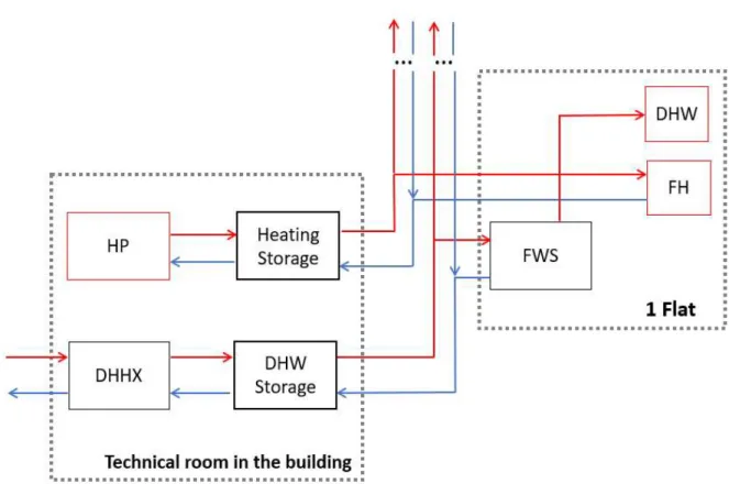
A 4-pipe distribution system has been studied to cover the heating demand and the DHW preparation: 2 pipes are used for the space heating with HP, while 2 pipes are used for the DHW. A scheme of the system is shown in Figure 4.
A Fresh Water Station (FWS) is placed in each flat in order to provide DHW. The hot source for the FWS is taken from a DHW storage in the technical room, heated up by the DH through
18
a district heating heat exchanger (DHHX). The space heating, provided by a heat pump, has not been investigated in this work, while DHW preparation from DH is subject of the study. The technical room is placed in the corner on the left-hand side of the building (see Figure 3). A system of pipes connects the technical room with each flat of the building. Building A has 96 flats and an average number of 2 people per flat is assumed for DHW calculation.
2.2.
Dynamic simulation tool.
The model for the DHW preparation has been developed in Matlab/Simulink environment in order to carry out dynamic simulations. A method to run a dynamic simulation for a big multi-family building, based on the flat-level DHW preparation model, is then developed.
A dynamic simulation is the first step to design energy-efficient buildings since it takes into account short time variables that would be neglected in a stationary simulation. Thus, the aim of a dynamic simulation is to draw out a set of results over time, which can help the decision-making process for the design of heating and DHW preparation systems. Short time variables are not only the one linked to the DHW usage (which can change second by second), but also all those variables linked to the thermal inertia of the components constituting the DHW preparation system. In Matlab/Simulink, every component of the system can be represented with its own thermal capacity.
Blocks representing hydraulic and thermodynamic components of a DHW production model are taken from the CARNOT ("Conventional And Renewable eNergy systems OpTimization") block-set library. All the blocks are connected in order to communicate with each other through transfer functions.
19
2.3.
Simulation models
2.3.1.
DHW preparation model, flat-level
The model developed in Matlab/Simulink has the purpose to simulate a system to produce DHW for a single flat. Each of the 96 flats of the building has its own FWS for DHW preparation. The study of the FWS in one flat is the starting point of this work: the flat-level HX can be rescaled in order to simulate the supply of DHW to 96 flats with a single central HX.
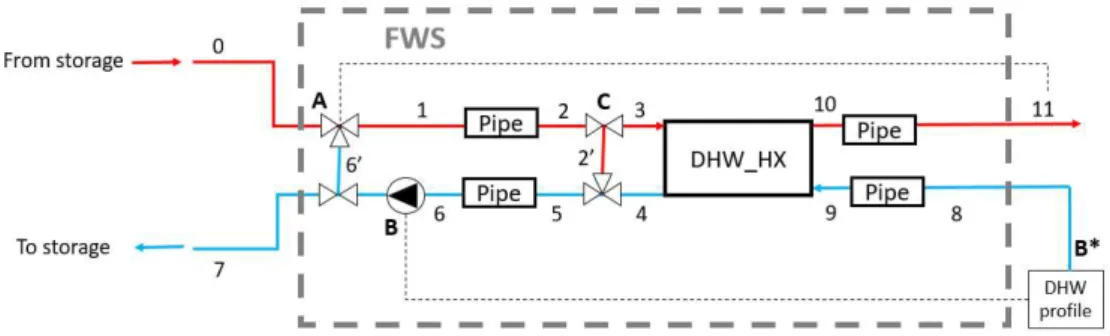
A simplified hydraulic scheme of the model is shown in Figure 5.
The hot water entering the FWS comes from a central thermal storage tank placed in the central technical room. In this tank, the energy to supply to all the flats of the building is stored as hot water. The temperature of the water coming from the storage (position 0 in Figure 5) is fixed. The first mixer-diverter (position A) has the purpose to control the required temperature of hot water supplied to the user (position 11) in order to always achieve the set point temperature. The second mixer-diverter (position C) works as a bypass for the HX. The system, in fact, is configurated in order to always have a minimum mass flow circulating in the primary side. A bypass of the HX is necessary when there is no mass flow in the secondary side. In this study, the value of the minimum mass flow has a fixed value. However, in reality, this mass flow should be controlled considering that the return temperature to the storage (after the thermal losses in the bypass pipe) should not be too high (around 35°C) in order to avoid high thermal losses in the return pipe to the storage.
Four pipe blocks are placed before and after the FWS in both sides. Pipe blocks are used to simulate thermal behaviour of the pipes and to get stability in the model.
20
The mass flow circulating in the secondary side is fixed by the DHW user profile (see 2.5). The mass flow circulating in the primary side, instead, is fixed by the circulation pump. The control on the pump is based on a logic linked to the user profile (see 2.4).
FWS includes a cross flow HX. In the primary side, the hot water comes from the storage. In the secondary side the cold water is heated up to the set point temperature.
2.3.2.
DHW preparation model, building-level
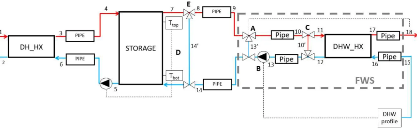
The development of the model for the building-level DHW preparation is based on the flat-level model. A single FWS simulates a central production of DHW for 96 flats. The hydraulic scheme of the model is shown in Figure 6.
The model can be divided into three branches: storage charging circuit (including positions from 3 to 6 in Figure 6), storage discharging circuit (including positions from 7 to 14), and user circuit (including positions from 15 to 18).
The DH heats up a thermal storage tank. The heat exchange between the water from the DH and the water circulating in the storage charging circuit is realized by a HX (so called district heating heat exchanger DHHX). The DHHX and the storage tank are in the same technical room and the length of the pipes is 3 m. A pump circulates the water in the storage charging circuit.
The storage tank is designed to be heated to 85°C by the hot water produced in the DHHX and it is sized in order to hold all the daily thermal energy required to produce DHW in the building.
21
Two temperature signals are used to control the circulation pump: Ttop (measured at the top of the tank) and Tbot (measured at the bottom of the tank).
The storage discharging circuit connects the storage tank to the FWS. In the reality, one FWS is placed in each flat. The sum of the length of the pipes that connect the storage to every single FWS placed in each flat, is equal to 426 m and it is assumed, in the simulation model, as the length of the connection between the storage tank and the central FWS.
Three mixer-diverter couples are used along this path to maintain the designed operative conditions for the HX. The first mixer-diverter (position E in Figure 6) is placed right after the storage tank and it aims to fix the temperature of the hot water out of the storage. The second mixer-diverter, included in the FWS (position A), acts as a controller on the temperature of the DHW supplied to the user (position 18). The third mixer-diverter (position C) is also included in the FWS and it acts as a bypass for the HX.
As already explained for the flat-level model, also for the building model, four pipe blocks are located before and after the HX in both sides to simulate thermal behaviour of the pipes and to get stability in the model.
The mass flow circulating in the user circuit is set according to the user profile. The user profile is also the input for the controller of the circulation pump in the storage discharging circuit (as it is explained in 2.4.4).
22
2.4.
Controllers
For the proper development of a model it is essential to well define the controllers. In a typical controller, a set of variables acts as an input for a system that manipulates these variables in order to get an output. The output is called “control signal” and it is used, in these models, as an input for mixers-diverters or pumps. It aims to set the so called “controlled variable” to a set point value.
The FWS model includes two controllers: user mixer-diverter control (position A in Figure 5 and in Figure 6) and storage discharging-pump control (position B in Figure 5 and in Figure 6). These two controllers are included in the FWS and so they are used for both the models: flat-level model and building-flat-level model. A user mass flow control is also used in the flat-flat-level model (position B* in Figure 5). The building-level model also includes the storage-charging pump control (position D in Figure 6) and storage mixer-diverter control (position E in Figure 6). In the next paragraphs, all these controllers are described.
2.4.1.
Storage charging-pump controller
This controller is used to set the mass flow in the storage charging circuit. The mass flow is controlled in order to always get the set point temperature in the whole storage tank. Thus, the control signal is an input for the storage charging pump and the controlled variable is the mass flow.
Two values of temperature are the inputs of the controller: the temperature Ttop of the water at the top of the storage tank, and the temperature Tbot of the water at the bottom of the tank. The scheme of the controller is shown in Figure 7.
23
These two values of temperature are then compared to the set point, giving a boolean output (1 or 0 if the comparison is, respectively, true or false). The boolean outputs from the comparison are the “input” and “reset” values of an integrator. The “input” signal is the value that is integrated. With regard to the “reset” value, every time the Ttop switches from Ttop < 85°C to Ttop ≥ 85°C, it switches from 0 to 1 and it resets the initial value of the integral to 0.
Two cases are presented in Table 1. In both cases Tbot is switching from a T < 85°C to T = 85°C, resetting the initial value to 0.
In Case 1 Ttop > 85°C. The “reset” signal fixes the initial condition of the integral back to 0: the output of the integral is 0 and stops the pump.
In Case 2 Ttop<85°C. The “reset” signal fixes the initial condition of the integral back to 0: the output of the integral is 1 and it activates the pump.
These two cases are summarised in Table 1.
Table 1: reaction of the control in two simple cases Ttop < 85°C Reset to initial condition Output
Case 1 0 Reset to 0 0
Case 2 1 Reset to 0 1
2.4.2.
Mixer-diverter controller
This is a temperature controller and it is used to limit the temperature of the water in certain branches of the circuit. The controller is composed by a mixer and diverter as it is shown in Figure 8.
24
The controlled variable is the temperature of the fluid that comes out from the mixer. The control signal is called fdiv and it is elaborated by the mixer, based on the difference between the temperature to control and a set point temperature as it is possible to see from the scheme in Figure 9.
The error is also multiplied by a constant called t1 and then integrated in order to create the fdiv signal. The smaller the constant t1, the sooner the system reaches the stability after the action of the control. fdiv is in the range between 0 and 1 and it acts on the diverter, setting the percentage of the fluid that is diverted to the mixer. The mass flows are set according to the following equations referred to the scheme in Figure 8
ṁ2 = ṁ1 · 𝑓𝑑𝑖𝑣 (1) ṁ3 = ṁ1 · (1 − 𝑓𝑑𝑖𝑣) (2)
One mixer-diverter controller (called storage mixer-diverter controller) is included in the building-level model and it is placed right after the storage in the storage discharging circuit (position D in Figure 6). The controlled temperature is the one of the water sent to the FWS. A mixer-diverter controller (called user mixer-diverter control) is also included in the FWS and so it is used in both the models (position A in Figure 5 and Figure 6). The controlled variable is the DHW supply temperature (position 11 in Figure 5 and position 18 in Figure 6). In this case, this temperature is controlled indirectly. The controller, in facts, does not changes directly the temperature of DHW supply, but it changes the temperature of the water entering the HX in the primary side (position 3 in Figure 5 and position 11 in Figure 6) in order to get the set point temperature in the DHW supply.
25
2.4.3.
Storage discharging-pump controller
This controller is used to set the mass flow in the storage discharging circuit. The value of this mass flow is set in order to provide, to the HX, the hot source to achieve the requests.
Thus, the control signal is an input for the storage discharging pump and the controlled variable is the mass flow. The control signal, in the range between 0 and 1, acts on the pump fixing the percentage of the design value of the mass flow circulating. Two different discharging-pump strategies are considered: on-off control and proportional control:
1) The on-off control takes as input the value of the mass flow defined by the user profile and fixes the control signal to 1 (if the user is asking for DHW) or to “minimum” (if the user is not asking for DHW). 1 means that 100% of the designed mass flow circulates in the storage-discharging circuit, while “minimum” means that the mass flow circulating is at a fixed minimum value.
2) The proportional control takes as input the value of the mass flow defined by the user profile. The controller elaborates an input signal on the pump that is between 1 and a minimum value. The signal 1 is obtained during the peak request and it fixes the mass flow on the storage-discharging circuit to the design value. When there is no DHW request by the user, the controller elaborates a minimum value for the input signal of the pump, in order to set the mass flow circulating in the circuit to a minimum value, ensuring the minimum mass flow circulating in the primary side of the FWS.
2.4.4.
User mass flow controller
This control is only used in the flat-level model and it aims to achieve the thermal energy request by the user (achievement of useful energy). The controller sets the duration of the tappings creating a user mass flow profile. The duration of each tapping is calculated with the following equation:
𝑑𝑢𝑟𝑎𝑡𝑖𝑜𝑛 =
ṁ· · (3)
Where Q [kWh/tapping] is the energy supplied to the user by each tapping; ṁ [kg/(s·tapping)] is the mass flow of each tapping based on the DHW profile; Δθ is the temperature difference
26
between the cold water and the set point of the supplied DHW. In the first seconds of tappings, the mass flow supplied is at a temperature lower than the set point. The energy supplied in these seconds is not counted as useful energy. It means that the duration of each tapping can be longer lasting than the duration required by the original profile. Based on the calculated duration of the tappings, a new mass flow profile is created.
A simplified scheme, considering the input and the output of the controller, is shown in Figure 10.
27
2.5.
DHW profiles
The DHW profile strictly depends on the behaviour of the occupants of the house. For flat-level model and for building-level model, different profiles are described, aiming to check the influence of the profile on the simulation results. The profiles are either based on the standard EN16147, profile M (where a daily tapping cycle is described), or created as stochastic profiles with DHWcalc tool.
2.5.1.
Standard EN16147
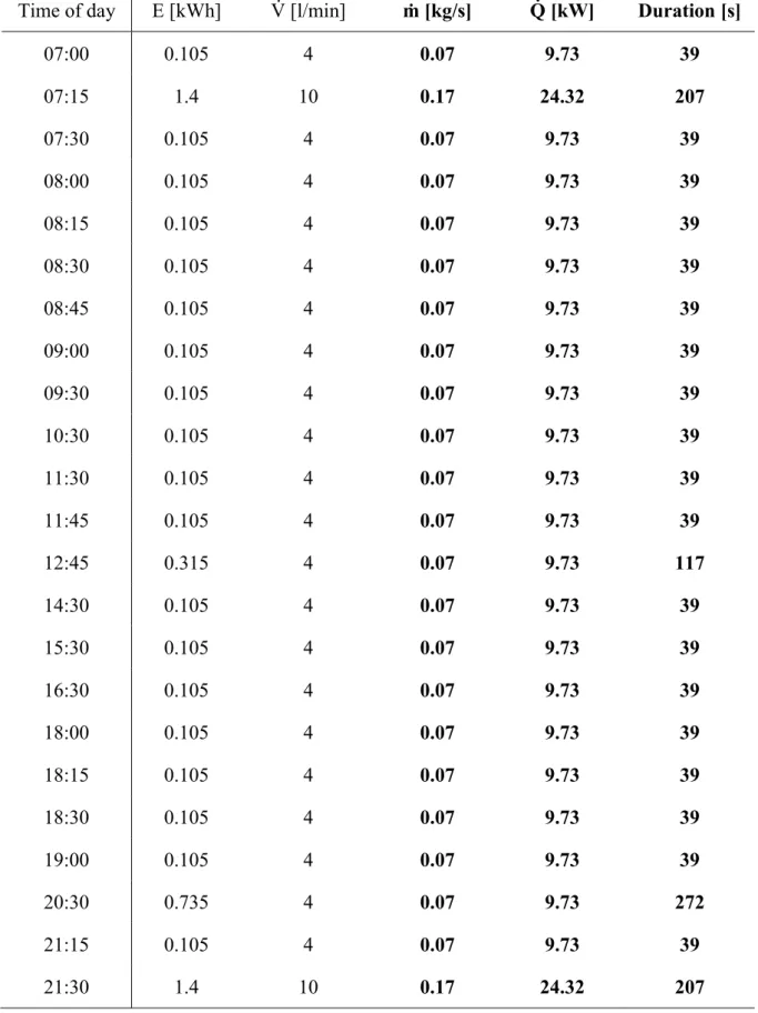
The standard EN16147 lists the tappings occurring during one day in a typical 4-people apartment. The profile M for the standard is considered. For each tapping, the starting time, the energy required and the volume flow are given.
The tapping cycle derived from the standard EN16147 includes three kinds of tappings: small tapping, shower (occurring twice per day) and dish washing. The mass flow [kg/s] from each tapping is derived by the volume flow listed in the standard EN16147 in l/min. The set point of the DHW supplied to the user is considered to be at 45°C while the cold water is considered to be at 10°C: Δθ = 35 °C. From Δθ and from the mass flow, it is possible to calculate the power associated to each tapping (Q̇) with Equation 14. Once the power of each tapping is calculated, it is divided by the energy given by the standard EN16147 in order to obtain the information about the duration of each tapping.
28
Table 2: daily tapping cycle based on the standard EN16147
Time of day E [kWh] V̇ [l/min] ṁ [kg/s] Q̇ [kW] Duration [s]
07:00 0.105 4 0.07 9.73 39 07:15 1.4 10 0.17 24.32 207 07:30 0.105 4 0.07 9.73 39 08:00 0.105 4 0.07 9.73 39 08:15 0.105 4 0.07 9.73 39 08:30 0.105 4 0.07 9.73 39 08:45 0.105 4 0.07 9.73 39 09:00 0.105 4 0.07 9.73 39 09:30 0.105 4 0.07 9.73 39 10:30 0.105 4 0.07 9.73 39 11:30 0.105 4 0.07 9.73 39 11:45 0.105 4 0.07 9.73 39 12:45 0.315 4 0.07 9.73 117 14:30 0.105 4 0.07 9.73 39 15:30 0.105 4 0.07 9.73 39 16:30 0.105 4 0.07 9.73 39 18:00 0.105 4 0.07 9.73 39 18:15 0.105 4 0.07 9.73 39 18:30 0.105 4 0.07 9.73 39 19:00 0.105 4 0.07 9.73 39 20:30 0.735 4 0.07 9.73 272 21:15 0.105 4 0.07 9.73 39 21:30 1.4 10 0.17 24.32 207
29
In the period between 21:30 and 7:00 no tappings occur. The value of the daily thermal energy request obtained from the standard EN16147 is the sum of the energy taken from each tapping and it is equal to 5.8 kWh/day (useful energy).
2.5.2.
Stochastic profile
A stochastic profile can be generated using DHWcalc tool. The profile is based on statistics, distributing DHW tappings throughout a fixed period, following a probability function. The user can set the reference conditions such as volume of DHW required daily, duration of the tappings, daily probabilities. Total mean daily draw-off volume in l/day is fixed according to the information derived from the standard EN16147. For a long period-simulation, probability seasonal variations, weekend variations and holiday periods can be set. The tool can be used to create either a profile per each flat separately or a profile for the whole building. The profiles are given as text files containing all the information related to the tappings.
2.5.3.
Simultaneity factor
In order to evaluate a building profile for the building-level DHW preparation model, one approach would be to consider the same DHW profile for all the flats. In this case the tappings for each flat would be considered occurring at the same time and the peak load for the building would be the sum of the peak load of each flat. However, in reality, the loads for every single flat do not occur at the same time. This is the reason why this approach cannot be considered. A simultaneity factor fs is taken into account in these simulations. The simultaneity factor is calculated as follow:
𝑓𝑠 = ∑
_
(4)
The denominator of the ratio is the sum of the maximum load daily asked by each flat. The numerator is the daily peak load of the building. As already mentioned, the peak loads for each flat do not occur at the same time, this is the reason why the building peak load differs from the sum of the flat peak loads. This difference changes according on how the building-level profile is implemented from the flat-level profile.
If the flat peak loads occur simultaneously, their sum is equal to the building peak load and fs is equal to 1, otherwise fs is lower than 1.
30
2.5.4.
Implemented DHW profiles
2.5.4.1. Flat-level
For the flat-level model, two DHW profiles are tested:
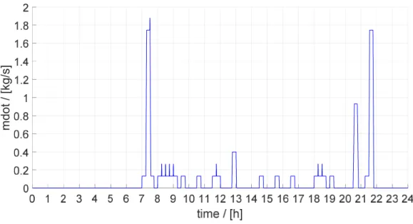
1) One profile derives from the standard EN16147 (profile M). With this DHW profile, 5.8 kWh/day is the daily useful energy requested by the user. Two peaks (0.17 kg/s) occur at 7:15 and 21:30 and they are due to the showers. The duration of the tappings has been already shown in Table 2. No tappings occur during the night between 21:30 and 7:00. The trend of this profile is shown in Figure 11.
Figure 11: DHW profile from standard EN 16147, single flat-level
m d o t / [k g/ s]
31
2) Stochastic profile derives from DHWcalc, considering 144 l/day as daily DHW draw-off volume, in order to supply 5.8 kWh/day of useful energy to the user. The profile is generated for one day and the tappings are randomly distributed all over the day. The mass flow of the first tapping occurring in the morning is equal to 0.42 kg/s. No tappings occur during the night between 22:30 and 7:00.
The trend of this profile is shown in Figure 12.
Figure 12: stochastic DHW profile, single flat-level
m d o t / [k g/ s]
32 2.5.4.2. Building-level
In order to simulate the influence of the DHW profiles on the results, four different building profiles are tested: two of them are derived from the standard EN16147, two are crated with DHWcalc.
An average number of two people per flat is considered for the creation of the building profiles. The four building DHW profiles are here listed:
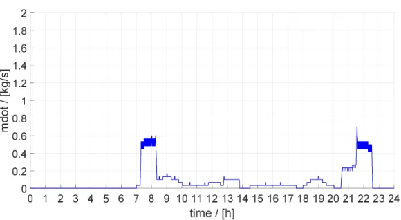
1) Hourly average profile. From standard EN16147, profile M, the energy requested of the building from each tapping is spread over one hour. The peak load for the DHW (occurring from 7:00 to 8:00 and from 21:00 to 22:00) is calculated assuming a simultaneity factor equal to 0.2 and the reduced energy in the peak power is added in the hour before the first peak (from 6:00 to 7:00) and after the last peak (from 22:00 to 23:00) (Dermentzis, 2019). The sum of the individual mass flow peaks is equal to 16.32 kg/s, while the value of the maximum mass flow with this profile is equal to 0.36 kg/s, then the simultaneity factor is 0.02. The resulting profile is shown in Figure 13.
Figure 13: hourly average profile, building-level
m do t / [k g/ s]
33
2) 10 seconds profile. The reference is the standard EN16147, profile M. A single flat profile is derived from the standard. In the implementation of the profile in the building model, a delay of 10 seconds on the starting time of the daily tapping routine of each flat is considered. It means that, if the first tapping for the first flat occurs at 7:00:00, the first tapping for the second flat occurs 10 s after, at 7:00:10. The first tapping for the 96th flat occurs after 960 s from the first one, at 7:16:00. The value of the maximum mass flow with this profile is equal to 1.91 kg/s. The simultaneity factor in this case is equal to 0.12.
This profile is shown in Figure 14.
Figure 14: 10 seconds profile, building-level
m do t / [k g/ s]
34
3) 39 seconds profile. Also in this case, a profile for a single flat is derived from the standard EN16147, profile M. The delay on the starting time of the daily tapping routine for each flat is 39 s, which is the duration of a small tapping (see Table 2). The starting time for the daily tapping routine of the first flat is 7:00:00, while the starting time for the 96th flat is 8:02:24. The value of the maximum mass flow with this profile is equal to 0.69 kg/s and the simultaneity factor is equal to 0.04. The profile is shown in Figure 15.
Figure 15: 39 seconds profile, building-level
m do t / [k g/ s]
35
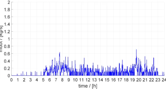
4) Stochastic profile. DHWcalc tool is used to generate a stochastic building profile. The profile is generated for one day and it spreads the daily tappings all over the day. The total draw-off volume per day is derived from the standard EN16147, multiplying the daily DHW volume used in a 2-people flat, for the number of flats of the building. The value of the maximum mass flow with this profile is equal to 0.70 kg/s. Also considering the sum of the individual mass flow peaks equal to 16.32 kg/s the simultaneity factor for this profile is equal to 0.04. The profile is shown in Figure 16.
Table 3 summarises the simultaneity factor for the four different building profiles.
Table 3: simultaneity factor with the four different building profiles Hourly average profile 10s profile 39s profile Stochastic profile
fs 0.02 0.12 0.04 0.04 m do t / [k g/ s]
36
2.6.
Parametrization of the models
2.6.1.
Flat-level model
A flat with 4 occupants, with a useful energy request equal to 5.8 kWh/day, is considered for the simulations. The temperature of the water coming from the storage is fixed at 52°C (position 0 in Figure 5). No storage is simulated in the flat-level model. The water in the secondary side of the HX is taken as cold water at 10°C (position 8 in Figure 5) and it is heated up to 45°C (position 11). The temperature of the water out of the HX in the primary side (position 4) is the only temperature that is not fixed.
A temperature not higher than 30°C is desirable for the water out of the HX in the primary side (position 4). This water, after the exchange, still holds thermal energy and it causes non-neglectable thermal losses in the return pipe to the storage tank.
The four 1-m pipes located in each branch of both sides of the FWS have a small capacity (100 J/(m·K)) and high thermal losses (5 W/(m·K)) so that, when there is no DHW request from the user, the water contained in these pipes reaches the room temperature (fixed at 20°C).
A 35-kW HX is chosen, based on common practise. Based on the characteristics derived from the data sheet of Danfoss, three parameters of the HX are calculated: the heat transfer coefficient between the two sides of the HX UAHX [W/K], the thermal capacity C [J/K] and the heat losses coefficient UAHL [W/K].
UAHX value is calculated with the following equation. UAHX=
̇
[ ] (5)
Where Q̇ is the power of the chosen HX, while Δθlog is calculated as follow: 𝛥𝜃 log = ( )
( ⁄ ) (6)
Where:
𝛥𝜃1 = 𝜃 _ − 𝜃 _ (7)
𝛥𝜃2 = 𝜃 _ − 𝜃 _ (8)
primary_in and primary_out are referred respectively to the inlet and outlet of the primary side HX, while secondary_in and secondary_out are referred to the inlet and outlet of the secondary side of the HX.
37
The thermal capacity C [J/K] is calculated with the following equation. 𝐶 = 𝑐𝑝 · 𝑚 (9)
Where cp is the thermal capacity of the stainless steel (cp_stainless_steel = 502 J/kgK) and m is the mass of the HX shown in Table 4.
Heat transfer coefficient with the ambient UAHL [W/K] is calculated from the thickness of the insulant s, its thermal conductivity λ and the total external surface S of the HX (listed in Table 4) with the following Equation 9.
𝑈𝐴 = · 𝑆 (10)
Figure 17 shows a simplified representation of the HX.
Table 4 summarizes the main characteristics of the HX chosen by the catalogue of Danfoss
Table 4: characteristics of the HX
Model of HX XB51L
A [m] 0.466
B [m] 0.256
C [m] 0.064
38
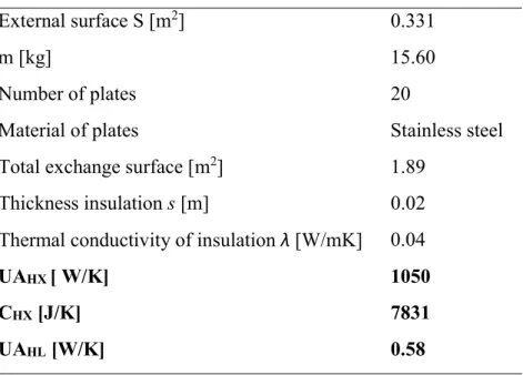
External surface S [m2] 0.331
m [kg] 15.60
Number of plates 20
Material of plates Stainless steel
Total exchange surface [m2] 1.89
Thickness insulation s [m] 0.02
Thermal conductivity of insulation λ [W/mK] 0.04
UAHX [ W/K] 1050
CHX [J/K] 7831
UAHL [W/K] 0.58
As already mentioned, two different user profiles are considered: the one given by the standard EN 16147 and the stochastic profile. Also, two different control for the circulation pump are tested: on-off and proportional control. Four different cases can be simulated, as shown in Table 5.
Table 5: single flat analysed cases Profile Pump control Case 1 EN 16147 On-Off Case 2 EN 16147 Proportional Case 3 Stochastic On-Off Case 4 Stochastic Proportional
In this model, no distribution system from/to the storage is considered, thus no considerations about thermal losses in the pipes can be made.
The model of the HX chosen from CARNOT library calculates the outlet temperatures referring on the inlet temperatures using the following equations taken from the CARNOT user guide:
θ _ = θ _ − 𝛹 · (θ _ − θ _ ) (11) θ _ = θ _ − · (θ _ − θ _ ) (12)
39
Where Ψ is a parameter called “dimensionless temperature change”, while W and W are the product between the mass flow and the capacity of the fluid in the two sides of the HX expressed in W/K.
2.6.2.
Building-level model
The daily thermal energy required by the building is equal to 280 kWh/day. This is the base data used to size the storage thermal tank which is simulated in the building model. The volume V [m3] of the storage tank, necessary to store the daily thermal energy, is calculated with the following equation.
𝑉 =
· · (13) Where:
Q = 280 kWh/day is the daily thermal energy stored in the tank; ρ = is the value of water density;
cp = is water specific heat capacity;
Δθ = is the temperature difference between the hot water filling the tank (position 4 in Figure 6) and the cold water leaving the tank (position 5 in Figure 6).
In respect to Equation 13, fixing Δθ = 60 K, a 4 m3 thermal storage tank is chosen. The diameter of the tank is supposed to be 2 m. The heat losses of the walls of the storage tank are taken from the PHPP and they are equal to 5.5 W/K. Geometrical and thermal characteristics of the tank are summarized in the Table 6.
Table 6: Geometrical and thermal characteristics of the storage tank Surface [m2] Heat losses coefficient [W/m2K]
Top cover 3.14 1.2
Bottom 3.14 1.2
Cylindrical surface 8 3.08
The set point temperature of the storage is constantly 85°C.
All the distribution pipes of the building are considered in a single pipe connecting the storage tank to the central HX. As already mentioned in 2.3.2, this pipe is considered to be 426 m
40
(Dermentzis, 2019). The diameter of the pipes is considered to be 3.5 cm. The insulation of the pipe is considered with a heat transfer to the ambient coefficient equal to 0.227 W/(m·K) (Dermentzis, 2019). The thermal capacity of the pipes is 1440 J/(m·K) as a typical value of thermal capacity of the pipes taken from data sheets. Four 1-m pipes (with high losses equal to 5 W/(m·K) and low thermal capacity of 100 J/(m·K)) are placed in each branch of the FWS in order to give stability to the systems and to let the fluid reach the temperature of the room while no mass flow is circulating.
For the storage-discharging pump control, only the proportional control is tested.
Once the user mass flow profile is predicted, the maximum load of the HX is fixed. From the peak of the DHW mass flow supplied to the user (and so the peak load), it is possible to calculate the power Q̇ [W] of the HX with the following equation.
𝑄̇ = ṁ · cp · Δθ (14)
Where:
- ṁ [kg/s] is the maximum DHW mass flow supplied to the user; - cp is the water thermal capacity;
- Δθ is the temperature difference between the cold water and the DHW supplied to the user.
The parametrization of the HX for the building is based on the peak loads: it gives different values depending on the chosen DHW profile and so on the simultaneity factor. Figure 18 shows the different building peak load obtained considering or not considering the simultaneity factor.
Building peak load [kW]
(Flat_peak_load x 96)
n of flats (Flat_peak_load x 96) x fs
96 0
41
Table 7 summarizes the 4 different user DHW profiles considered in this work for the building-level model, with the simultaneity factor associated to each profile and the calculated values of Q̇ (Equation 13) and UAHX (Equation 4) of the HX.
Table 7: list of user profiles with fs and calculate values of Q̇ and UAHX for each profile.
Name of the profile Maximum ṁ [kg/s] fs Q̇
[kW]
UAHX [W/K]
Case 1: Hourly average profile 0.37 0.02 53 4280
Case 2: 10 seconds profile 1.91 0.12 280 22612
Case 3: 39 seconds profile 0.69 0.04 101 8156
Case 4: Stochastic profile 0.71 0.04 104 8399
Based on Table 7 it is possible to parametrize the HX in four cases which differ with respect to the user DHW profile. In each case, a different value of thermal capacity of the HX is calculated, in order to approximate a realistic behaviour of 96 HXs together. The parametrization of the HX in each case is summarised in Table 8.
Table 8: characteristics of the HX in each case
Characteristics Case 1 Case 2 Case 3 Case 4
Model of HX XB51L XB51L XB51L XB51L A [m] 0.466 0.466 0.466 0.466 B [m] 0.256 0.256 0.256 0.256 C [m] 0.106 0.220 0.142 0.142 External surface S [m2] 0.392 0.556 0.444 0.444 m [kg] 21.68 38.40 27 27 Number of plates 36 80 50 50
Material of plates Stainless steel Stainless steel Stainless steel Stainless steel Total exchange surface S [m2] 3.57 8.19 5.04 5.04 Thickness insulation s [m] 0.02 0.02 0.02 0.02 Thermal conductivity of insulation
λ [W/mK] 0.04 0.04 0.04 0.04 CHX [J/K] 10883 19277 13554 13554 UAHL [W/K] 0.69 0.97 0.78 0.78 A B C
42
Chapter 3. Results
The following key performance indicators are considered:
Useful energy UE, i.e. the amount of energy supplied to the user; Final energy FE, i.e. the energy taken from the DH;
Losses, as the difference between FE and UE;
θDHW, i.e. the temperature of the water supplied to the user;
θreturn, i.e. the temperature of the water sent back to the storage from the FWS;
Waiting time, i.e. the time that the DHW needs to reach the set point temperature, as it is shown in Figure 19.
43
For the flat-level DHW production model, the logic of the control of the pump and the DHW profiles are the variables for the simulations. The simulations aim to get information about the achievement of the required useful energy and about the comfort which includes analysis of the temperature development and the dynamic behaviour as it is shown in the scheme in Figure 20.
For the building-level DHW preparation model, DHW profiles and the size of the HX are the variables for the simulations. The results regarding the achievement of the required useful energy, the temperature development and the dynamic behaviour allow to evaluate the comfort. The return temperature to the storage is analysed. With the building-level DHW preparation model, the temperature development also allows to get information about the pipe losses, as it is shown in Figure 21.
Figure 20: scheme of the methodology used in the flat-level simulations
44
3.1.
Results of the flat-level model
Table 9 summarises the simulation cases for the flat-level DHW preparation.
Table 9: simulation cases for flat-level DHW preparation FLAT-LEVEL
Case 1 Standard EN16147 profile + on-off control Case 2 Standard EN16147 profile + proportional control Case 3 Stochastic profile + on-off control
Case 4 Stochastic profile + proportional control
According to Table 9 the DHW profile and the logic of the control of the pump varies in the 4 cases, while the parametrization of the HX does not change in the 4 cases.
Referring to Figure 5 the following temperatures are analysed: water from storage, “From_storage”, position 0;
water entering in the primary side of the HX, “Pri_in”, position 3; water going out from the primary side of the HX, “Pri_out”, position 4; water entering in the secondary side of the HX, “Sec_in”, position 9; DHW temperature, “Sec_out”, position 11;
water to storage, “To_storage”, position 7.
The trend of the mass flow circulating in the FWS is also analysed, referring to Figure 5: mass flow circulating in the primary side of the HX, “primary”;
mass flow circulating in the secondary side of the HX, “secondary”; mass flow diverted by the mixer-diverter control, “diverted”, position 6’;
45
3.1.1.
Energy evaluation
Table 10 shows the useful energy for each case.
Table 10: useful energy in the 4 cases for the flat-level DHW preparation Case 1 Case 2 Case 3 Case 4 Useful energy [kWh/day] 5.85 5.85 5.85 5.89
As it is possible to see, the daily amount of useful energy for DHW is achieved in each case, showing that the HX is well parametrized for these operative conditions.
46
3.1.2.
Comfort
Temperature development
The daily development of the temperatures can help to understand the influence of the DHW profile and of the logic of control on the behaviour of the HX. Figure 22 shows the temperatures development and the mass flows primary, secondary and diverted for case 1.
The temperature From_storage of the water coming from the storage is fixed at 52°C. This water either circulates in the primary side of the HX or bypasses the HX when there is no request by the user.
In the period between 00:00 and 7:00, no mass flow enters the HX and so the temperature Pri_in of the water entering the HX reaches the room temperature which is 20°C.
In order to have a more understandable representation of these trends, the period between 6:48 and 9:12 is shown in Figure 23. In this period a maximum load (due to the shower) and some small peaks occur.
Figure 22: temperatures of the system and mass flow circulating in FWS in case 1 during one day
/ [° C ] m do t / [k g/ s]
47
During the tappings, the hot water from the storage enters the HX. The temperature of the water entering the HX in the primary side (Pri_in), changes from the temperature of the room to the temperature of the water coming from the storage. Once the tapping stops, this temperature decreases, reaching again the temperature of the room, with a delay due to the capacity of the HX.
When a tapping occurs, the mass flow circulating in the primary side of the HX is fixed at 0,38 kg/s. The higher the mass flow of the DHW supplied to the user, the lower the temperature of the water going out from the HX in the primary side (Pri_out).
For long periods without tappings, the temperature of the water out of the HX in the secondary side (Sec_out) reaches the temperature of the room with a certain delay also due to the thermal capacity of the HX. As soon as a tapping starts, this temperature increases reaching a peak temperature that is higher than the set point, here fixed at 45°C. This is the reason why a user mixer-diverter control is needed. With a certain delay, the control stabilizes this temperature at the set point.
When the hot water bypasses the HX, it is reduced by the heat losses in the bypass pipe. In this case the temperature of the water sent back to the storage (To_storage) slightly differs from the temperature of the water coming from the storage (From_storage). When the hot water
Figure 23: temperatures of the system and mass flow circulating in FWS in case 1 from 6:48 to 9:12 / [° C ] m do t / [k g/ s]
48
circulates in the HX, instead, it is reduced by the heat exchanged with the cold water circulating in the secondary side. In this case it is desirable to have a lower temperature of the water sent back to the storage, in order to reduce the losses in the return pipe. The logic of the control used in each case, influences this temperature.
The same period between 6:48 and 9:12 is represented in Figure 24 for case 2.
The discussion about the development of the temperatures for case 1 is still valid for case 2. The two cases differ on the mass flow circulating in the primary side of the HX (primary) that, in case 2, assumes different values according to the mass flow circulating in the secondary side (secondary). For the trend of the temperatures of the water coming from the storage, the water entering the HX in both the sides and the DHW supplied to the user (respectively: From_storage, Pri_in, Sec_in and Sec_out), no differences are observed in case 1 and case 2. The temperature development of the water leaving the HX in the primary side (Pri_out) and of the water sent back to the storage (To_storage), instead, is different for the two cases. For the first peak represented in Figure 23 and Figure 24, the mass flow circulating in the primary side of the HX (primary) is lower in case 2 than in case 1. It means that less energy is supplied to the HX during this peak and so that the temperature leaving the HX from the primary side (Pri_out) is also lower in case 2 than in case 1. During the tapping, the temperature leaving the
/ [° C ] m do t / [k g/ s]
Figure 24: temperatures of the system and mass flow circulating in FWS in case 2 from 6:48 to 9:12
49
HX from the primary side and the temperature of the water sent back to the storage are the same. This is also true for all the small tappings occurring in the examined period. For the big tapping occurring at 7:15, the mass flow circulating in the primary side (primary) is the same in case 1 and case 2. Also the temperature leaving the HX from the primary side and the temperature of the water sent back to the storage are the same for the big tapping.
The comparison between the temperature of the water sent back to the storage (To_storage) in case 1 and in case 2 is represented in Figure 25 in the period between 6:48 and 9:12.
The comparison between the temperature of the DHW supplied to the user (Sec_out) in case 1 and in case 2 is represented in Figure 26 in the period between 6:48 and 9:12.
/
[°
C
]
Figure 25: comparison of the temperature sent back to the storage for case 1 and case 2 in the period between 6:48 and 9:12
50
Figure 27 shows the temperatures development and the mass flows circulating in both the sides of the HX (primary, secondary) and the mass flow diverted by the mixer-diverter control (diverted ) for case 3 during one day.
/ [° C ] m do t / [k g/ s]
Figure 27: temperatures of the system and mass flow circulating in FWS in case 3 during one day
/
[°
C
]
Figure 26: comparison between the temperature of the DHW supplied to the user for case 1 and case 2 in the period between 6:48 and 9:12
51
The considerations about the trend of the temperature of the water from the storage and of the water entering the storage in the primary side, made for case 1, are still valid for case 3. The temperature From_storage of the water coming from the storage is fixed at 52°C: this water either circulates in the primary side of the HX or bypasses the HX when there is no request by the user.
In the period between 00:00 and 7:00, no mass flow enters the HX and so the temperature of the water entering the HX in the primary side (Pri_in) reaches the room temperature which is 20°C.
Also in this case, the period between 6:48 and 9:12 is represented in Figure 28. In this period, a maximum peak occurs with a long tapping between 7:00 and 7:12, and two other lower tappings occur later on.
The mass flow primary circulating in the primary side, during the tappings, is always equal to 0,38 kg/s. In the first big tapping occurring in the morning, the mass flow secondary, circulating in the secondary side, changes throughout the duration of the tapping assuming values that are even higher than 0,38 kg/s. For this tapping, the temperature Pri_out entering the HX, and so the temperature of the water sent back to the storage (To_storage), reaches a value that is lower
/ [° C ] m do t / [k g /s ]
Figure 28: temperatures of the system and mass flow circulating in FWS in case 2 from 6:48 to 9:12
52
than 30°C and this would be good in order to reduce the losses in the return pipe to the storage. However, the set point temperature of the DHW provided to the user (Sec_out) is not achieved. This temperature reaches only 42°C.
The same period between 6:48 and 9:12 is represented in Figure 29 for case 4.
With a proportional control, the mass flow circulating in the primary side of the HX (primary) in the first tapping occurring in the morning in case 4 is higher than in case 3. During this tapping, in case 4, the set point of the DHW supplied to the user (Sec_ou) (fixed at 45°C) is achieved. However, the temperature Pri_out entering the HX in the primary side, and so the temperature To_storage of the water sent back to the storage, during this tapping in case 4 are higher than in case 3. For the other three tappings represented in Figure 28 an Figure 29, the temperature Pri_out and To_storage in case 4 are lower than in case 3.
The comparison of the temperature To_storage of the water sent back to the storage in case 3 and case 4 is presented in Figure 30 for the period between 6:48 and 9:12.
/ [° C ] m do t / [ kg /s ]
Figure 29: temperatures of the system and mass flow circulating in FWS in case 4 from 6:48 to 9:12
53
From the comparison between case 3 and case 4 it is possible to see that on-off control does not guarantee the set point temperature of the DHW supplied to the user (Sec_out) in the big tapping occurring in the morning for the stochastic profile derived from DHWcalc. Furthermore, for the small tappings spread all over the day, the proportional control allows to have a lower temperature of the water sent back to the storage.
The comparison between the temperature of the DHW supplied to the user (Sec_out) in case 3 and in case 4 is represented in Figure 31 in the period between 6:48 and 9:12.
/
[°
C
]
Figure 30: comparison of the temperature sent back to the storage for case 3 and case 4 in the period between 6:48 and 9:12

![Table 6: Geometrical and thermal characteristics of the storage tank Surface [m 2 ] Heat losses coefficient [W/m 2 K]](https://thumb-eu.123doks.com/thumbv2/123dokorg/7397502.97525/39.892.171.721.910.1034/table-geometrical-thermal-characteristics-storage-surface-losses-coefficient.webp)
