A next-best-smell approach for remote gas detection with a mobile robot

(1)

POLITECNICO DI MILANO

Corso di Laurea Magistrale in Ingegneria Informatica Dipartimento di Elettronica, Informazione e Bioingeneria

A NEXT-BEST-SMELL APPROACH

FOR REMOTE GAS DETECTION

WITH A MOBILE ROBOT

Relatore: Prof. Francesco Amigoni Correlatore: Dr. Erik Schaffernicht

Tesi di Laurea Magistrale di: Riccardo Polvara, matricola 817572 Marco Trabattoni, matricola 823346

(2)

(3)

(4)

(5)

List of Figures

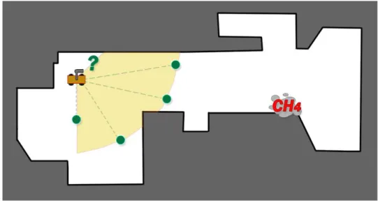
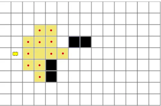
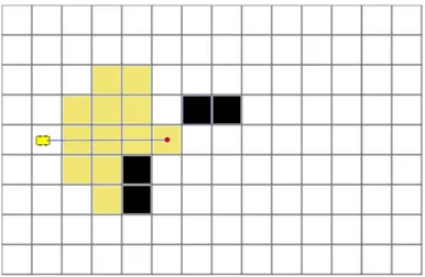
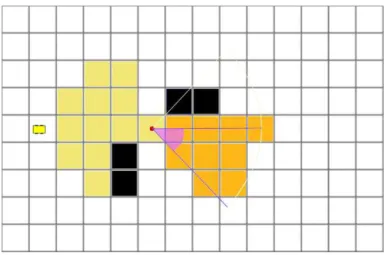
1.1 The Next-Best-Smell algorithm identifies, on the frontier

sep-arating explored and unexplored area, the next pose the robot has to reach combining in a single utility function different criteria. . . 2 2.1 Because the flexibility they can offer, mobile robots (left)

rep-resent an important innovation in a dangerous task like the gas detection one. In the first years they were combined with in-situ gas sensors (right), whose limitation is the fact they

have to be in direct contact with the gas to perceive it. . . 6

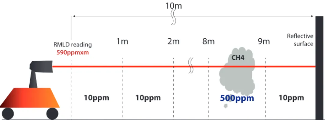
2.2 The Remote Methane Leak Detector is a TDLAS sensor which

can report the integral concentration of methan along its laser

beam (parts per million x meter) . . . 6

2.3 Next-Best-View system: acquire a partial map of the

sur-rounding environment, integrate it with the global map, iden-tify the new position to reach and then reach it. These steps

are usually reiterated until full coverage is achieved. . . 7

2.4 Different approaches were suggested in the field of map

cov-erage but most of them were not theoretically-grounded. For this reason Multi Criteria Decision Making was introduced with promising results. . . 8

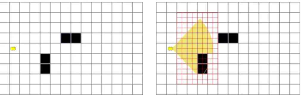
3.1 Grids representing the environment. We can see how when

performing a sensing operation (figure on the right) a grid with a higher resolution is used . . . 12

3.2 Candidate positions (marked with red dots) are the cells on

the boundary between the scanned and unscanned portion of the environment. . . 13

3.3 Travel distance criterion is computed as the distance between

the current robot position and the candidate pose. . . 14

(8)

3.4 Information gain criterion is computed as the number of free unscanned cells that the robot will be able to perceive from the candidate pose. . . 15

3.5 Sensing time criterion is computed as the scan angle required

to sense all the free unscanned cells visible from the candidate pose in the sensing operation (φmax - φmin). . . 15

4.1 After checking the termination condition, the robot scans the

surrounding environment, identifies new candidate positions and, after having evaluated them, selects the best one. These steps are iterated untill the full coverage is reached. . . 20 4.2 The three criteria are calculated with different techniques: ray

casting is used to estimate the value of information gain and

sensing time, while A* is implemented for the travel distance. 21

4.3 Ray casting used to calculate the value of information gain

of a candidate pose. When a ray reaches the center of a free cell, the information gain value is increased. . . 23

4.4 The information gain of a candidate pose is the number of

visible free unscanned cells. . . 24

4.5 The sensing time of a candidate pose is the angle between

the first and last rays shot to scan all the free unscanned cells visible from that pose. . . 24

4.6 The initial pose of the robot and the target cells. Different

weights are assigned to orthogonal and diagonal cells. . . 27

4.7 The cumulative costs are spread from the starting point to

the goal one, expainding always in the tree the node with the smallest value. . . 28

4.8 The shortest path is found proceeding backwards from the

goal and selecting each time the cell with the minimum f (n) value. . . 28

4.9 The backtracking operations is performed modeling a search

problem with a depth-first search algorithm. . . 29

4.10 Structure of the tree built during the navigation. Every time the robot reach a new position, this is add in the free with a list of all frontiers visible from there . . . 30 4.11 Every time the robot can not find any further frontiers in

front of it, it comes back to the previous pose and try to

(9)

5.1 Sensing positions identified during the exploration of the Freiburg University’s map using Configuration K, 15 meters for the gas

sensor range and 180 degrees for the scan angle φ. . . 40

5.2 Coverage ratio during the exploration of the Freiburg Uni-versity’s map using Configuration K, 15 meters for the gas sensor range and 180 degrees for the scan angle φ. . . 41

5.3 Sensing positions identified during the exploration of the Teknikhuset corridor’s map using Configuration M, 15 meters for the gas sensor range and 180 degrees for the scan angle φ. . . 42

5.4 Coverage ratio during the exploration of the Teknikhuset cor-ridor’s map using Configuration M, 15 meters for the gas sen-sor range and 180 degrees for the scan angle φ. . . 43

5.5 Husky A200 (Clearpath Robotics) equipped with a Lidar scan-ner, a pan-tilt unit and a TDLAS sensor for remote gas detec-tion. Methane leaks are simulated in the environment with some bottles filled with the gas . . . 44

5.6 Sensing positions obtained during the experiment in the real world using 10 meters for the gas sensor range and 180 degrees for the scan angle φ. . . 44

5.7 The weights assigned to the three criteria are shown on the simplex surface. Experimental activities demonstrated the the upper part of the simplex represent the locus of point offering a better overall performance. . . 49

5.8 Sensing positions obtained with the offline algorithm using only 4 directions, 90 degrees for the scan angle φ and a gas sensor range of 10 meters. . . 50

5.9 Sensing positions obtained with the online algorithm using only 4 directions, 90 degrees for the scan angle φ and a gas sensor range of 10 meters. . . 50

5.10 Sensing positions obtained with the online algorithm using 8 directions, 180 degrees for the scan angle φ and a gas sensor range of 10 meters. . . 50

A.1 Navigation stack tf tree (wiki.ros.org) . . . . 60

A.2 Example of a tf transform (wiki.ros.org) . . . . 61

A.3 Tf tree of the Husky robot used in our experiments . . . 62

(10)

(11)

List of Tables

3.1 Example of candidate evaluation with MCDM. . . 17

5.1 Criteria configuration - Weights assigned to each criterion and

coalitions among them. A coalition is defined as a subset of the criteria involved in the evaluation. . . 39

5.2 Results for Freiburg University map for each considered

con-figuration. In only two cases among thirteen the exploration was not totally completed. . . 39

5.3 Results for Teknikhuset corridor map for each considered

con-figuration. The full coverage was completed in all the tests. . 42

5.4 Comparison between the results obtained with the experiment

in the real world and the ones in simulations, using the same configuration and the same map. The different number of

total cells depend on the discretization process inside ROS. . 45

5.5 Having 8 directions instead of 4 among to choose can

repre-sent either an advantage (with tight spaces like in the Teknikhuset’s corridor, on the right) either a disadvantage (with open spaces

like in the Freiburg example, on the left). . . 47

5.6 The adoption of a pruning factor speeds up the convergence

of our algorithm but decrease the total amount of area we can cover. . . 47

5.7 Assigned a coverage constraint to satisfy, an higher

prun-ing factor can speed up the convergence speed of Next-Best-Smell, but in some cases (if a full coverage is required) it could

prevent to complete the task. . . 48

5.8 Comparison between offline and online approach. Two

con-figurations are reported for the online: 4 orientations with 90 degrees for the scan angle φ for the first and 8 orientations

(12)

(13)

List of Listings

4.1 Ray caster pseudocode . . . 22

4.2 A* pseudocode . . . 26

4.3 Subscription ot map server node to the the global costmap of the environment . . . 31

4.4 Sensing a MoveBaseGoal message to move the robot to the next pose . . . 32

4.5 Retrieving the exact pose of the pan-tilt unit before perform-ing a scannperform-ing operation . . . 33

4.6 Sending the right parameter to ptu control node to perform a scanning operation . . . 34

A.1 An example of nav msgs/Odometry . . . 63

A.2 Code used to get from tf the exact pose of the robot . . . 63

A.3 An example of YAML file . . . 64

(14)

(15)

Abstract

The problem of gas detection is relevant to many real-world applications, such as leak detection in industrial settings and landfill monitoring. In this thesis we address the problem of gas detection in large areas with a mobile robotic platform equipped with a remote gas sensor. We propose an online algorithm based on the concept of Next-Best View for solving the coverage problem to which the gas detection problem can be reduced. To demonstrate the applicability of our method to real-world environments, we performed a large number of experiments, both in simulation and in a real environment. Our approach proves to be highly efficient in terms of computational requirements and to achieve good performance.

(16)

(17)

Sommario

Il problema legato al rilevamento del gas `e di fondamentale importanza in molte applicazioni, quali l’identificazione delle perdite in ambienti industri-ali e il monitoraggio delle discariche. In questa tesi affrontiamo il problema del rilevamento del gas in ampi spazi interni con una piattaforma robotica mobile, equipaggiata con un sensore gas remoto. Proponiamo un algoritmo online basato sul concetto di Next-Best-View per risolvere il problema di copertura a cui il problema del rilevamento del gas pu`o essere ridotto. Per

dimostrare l’applicabilit`a del nostro metodo abbiamo svolto un elevato

nu-mero di esperimenti, sia simulati che in un ambiente reale. Il nostro ap-proccio ha dato prova di essere altamente efficiente in termini di risorse computazionali, e di raggiungere buone prestazioni.

(18)

(19)

Aknowledgment

Firstly, I would like to express my sincere gratitude to my advisors Prof. Francesco Amigoni and Dr. Erik Schaffernicht, for support while I was working on my Master thesis and the associated article, for their patience, motivation, and immense knowledge. Their guidance helped me during the time of research and writing of this thesis.

My sincere thanks also goes to Prof. Achim Lilienthal, who provided me an opportunity to join his team, and who gave access to the laboratory and research facilities. Without his precious support it would not be possible to complete this work.

I thank my fellow labmates Tomek, Malcolm, Ravi, Chit and Han for the stimulating discussions, for the sleepless nights we were working together before my departure, and for all the fun we have had in the five months spent in ¨Orebro.

Last but not the least, I would like to thank my family: my parents and my sister, for supporting me spiritually throughout writing this thesis and my life in general.

(20)

(21)

Chapter 1

Introduction

Recent advances in mobile robotics showed that the employment of au-tonomous mobile robots can be an effective technique to deal with tasks that are difficult or dangerous for humans. Examples include map exploration, map coverage, search and rescue, and surveillance. Fundamental issues in-volved in the development of autonomous robots span through locomotion, sensing, localization, and navigation. One of the most challenging problems is the definition of navigation strategies. A navigation strategy can be gen-erally defined as the set of techniques that allow a robot to autonomously decide where to move in the environment in order to accomplish a given task.

In the last years robot olfaction, a branch of robotics that combines gas sensors with the freedom of maneuver of mobile robots, has attracted more and more interest [30]. This interested has further increased with the birth of remote sensors which, unlike in-situ ones that must come directly into contact with the gas to be able to perceive it, allow to perform scans of the environment from considerable distances [7, 11], up to a couple of tens of meters, as in the case of TDLAS sensor, based on the spectroscopy analysis of the wavelengths of a laser [22, 14]. Because of their large size and cost it is virtually impossible to adopt a distributed solution with multiple sensors of this type in order to cover an environment, and therefore it has been tried to integrate this technology with mobile robots.

In this thesis we focus on the problem of gas detection in large environ-ments, like an office or a corridor with multiple rooms, calculating a path to cover all the area and to gain a complete mapping of the detected gas. Our approach is online, namely it incrementally perceives the environment and makes decisions on the basis of the knowledge obtained so far rather than a priori like happens with an offline strategy (Figure 1.1).

(22)

Figure 1.1: The Next-Best-Smell algorithm identifies, on the frontier separating explored and unexplored area, the next pose the robot has to reach combining in a single utility function different criteria.

In more details, we propose a Next-Best-Smell algorithm that exploits

Multi-Criteria-Decision-Making (MCDM) [3] to combine different criteria in

order to decide the next position the robot should reach to cover the envi-ronment with its remote gas sensor. After having reached the last position chosen, the robot acquires a new partial map, integrates it with the global map saved in his memory, decides the next location and reaches it, and repeat the steps above until it reachs an acceptable level of coverage. Can-didate locations are identified among multiple points on the frontier dividing scanned and unscanned space. In MCDM a robot evaluates the candidate locations in a partially explored environment according to an utility function that combines different criteria (for example, the distance of the candidate location from the robot and the expected amount of new information ac-quirable from there). Criteria are combined in a way that accounts for their synergy and redundancy.

The proposed approach seems to be promising: results reported in the following sections demonstrate that, because of the greedy nature of the Next-Best-Smell algorithm it is possible to cover most part of the environ-ment (a percentage around 80-90%) in relatevely few rounds, usually half of the ones required for a full coverage, but sometimes also less. For this reason it can represent an interesting solution in the field of gas detection where gas doesn’t remain near the source but moves around in the environment. These results are confirmed also by a simulated comparison made with an

(23)

offline approach, in which our algorithm obtained good performance, really close to the other’s ones in some circumstances.

The structure of this thesis is as follows: first of all (Chapter 2) we il-lustrate the current state of the art for what concerns gas detection and online navigation, then we will define the problem we want to solve and our solution proposal (Chapter 3). After having defined the architecture of our system (Chapter 4), we will report the results of our experiments (Chap-ter 5), performed both in simulation and with a physical platform, and the

comparison with an offline approach developed at MRO Lab at ¨Orebro

Uni-versity. In the end (Chapter 6) we summarize our approach, highlighting the main concepts, its advantages, and future works.

(24)

(25)

Chapter 2

State of the art

The idea of adopting online exploration strategies represents a novel ap-proach in the field of mobile robotic olfaction. Due to the lack of literature we split the current chapter in two parts, the first one aiming to illustrate the main techniques used until now for gas detection and the second one dedicated to online navigation.

2.1 Robot olfaction

Stationary networks of gas sensors represented until some years ago the most spread technique for gas detection, especially in situation of pollution monitoring [31]. The main particularity of this choice was the utilization of sensors defined in situ [23] because they should be in direct contact with the gas to perceive it. This represents a strong limitation because it poses the problem of their initial positioning and how they should be moved after some changes in the environment.

Recently, interest started growing towards mobile robot olfaction, a novel approach for gas detection using a mobile platform, with all the advantages that it can offer [21, 20].

The first step was combining mobile robots with in situ sensors (Figure 2.1), and this solution was used for mapping gas distribution [9, 8] and leak detection [25, 11]. The problem about this approach is that the robot still moved between predefined positions, along a path that should be recom-puted after changes in the environment, as for the static networks.

One of the biggest contributions in this field was represented by the adoption of Tunable Diode Laser Absorption Spectroscopy (TDLAS) sen-sors, able to perform remote measurements up to a limited range ( ∼ 30, 50

(26)

Figure 2.1: Because the flexibility they can offer, mobile robots (left) represent an important innovation in a dangerous task like the gas detection one. In the first years they were combined with in-situ gas sensors (right), whose limitation is the fact they have to be in direct contact with the gas to perceive it.

10ppm 10ppm 500ppm 10ppm 1m 10m 2m 8m 9m Reflectivesurface RMLD reading 590ppmxm CH4

Figure 2.2: The Remote Methane Leak Detector is a TDLAS sensor which can report the integral concentration of methan along its laser beam (parts per million x meter)

meters) [8], as shown in Figure 2.2. Because performing a scanning oper-ation is an extremely time consuming operoper-ation and the robot’s battery is limited, it became really important to find a path minimizing the number of times in which the robot stopped to sense for gas.

2.2 Exploration strategies

In general, almost all navigation strategies take as input a state enclosing information about the environment and provide as output the next location reachable by the robot. The way in which this process is performed allows to distinguish two class: offline and online strategies. In the first case, the set of possible destinations is computed for every possible input state before the beginning of the exploration task. With an online strategy, instead, the decision is computed during the task execution for the different situations the robot encounters.

(27)

ACQUISITION INTEGRATION SELECTION MOTION

Figure 2.3: Next-Best-View system: acquire a partial map of the surrounding environ-ment, integrate it with the global map, identify the new position to reach and then reach it. These steps are usually reiterated until full coverage is achieved.

criteria, each one with its own importance that can vary according to our scope. For example, one could search for the strategy minimizing the time spent in exploration while another for the one minimizing the total distance travelled by the robot. But sometimes a combination of these criteria can also be desirable.

Following the idea proposed by the offline strategy, some approaches were suggested in the mobile olfaction field but the most promising seems to be the one proposed by Arain et al. in [6], as extension of the work of Tamioka

et al [28], based on the combination of the Art Gallery Problem and the Travelling Salesman Problem: first of all they identify all the positions from

which the robot is able to see all the environment and then they calculate the minimum path connecting all these positions. In this way Arain et al. are able to find a closely optimal solution to cover all the environment and therefore detect any possible gas leak.

Starting from the assumption that gases move in the environment, our contribution in this thesis is a new approach that takes inspiration from the online strategy for map building, where the environment is usually unknown at the beginning and the robot has to incrementally discover it.

This kind of strategies usually follows the repetition of simple steps, reported in Figure 2.3: sensing the surrounding environment to build a partial map, integrating it with the current global map, selecting the next observation location, and reaching it.

An important feature of these systems, called Next-Best-View (NBV) systems, is how to choose the next observation location among a set of candidate locations, evaluating them according to some criteria. Usually, in NBV systems, candidate locations are chosen in such a way that they are on the frontier between the already explored free space and the unknown one [32], and they should be reachable from the current position of the robot.

During the evaluation phase of a candidate position, different criteria can be used and combined in diffent ways. A simple one is the travelling

cost [33], according to which the best observaton location is the nearest one.

Other works combine the travelling cost with expected information gain, 7

(28)

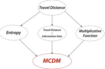
MCDM

Entropy

Travel Distance+

Information Gain

Multiplicative Function

Travel Distance

Figure 2.4: Different approaches were suggested in the field of map coverage but most of them were not theoretically-grounded. For this reason Multi Criteria Decision Making was introduced with promising results.

that is the expected amount of new information about the environment the robot can acquire performing a sensing action from the candidate location p. Given a candidate location p and called c(p) and A(p) the travelling cost and

the expected information gain, respectively, Gonz´ales-Ba˜nos and Latombe

[15] combine these two criteria with an ad hoc function in order to compute an overall utility (λ weighs the travelling cost and the information gain):

u(p) = A(p)e−λc(p) (2.1)

Similar criteria were considered also by Stachniss and Burgard [27], where the cost of reaching a candidate locations p, measured as the distance d(p) from the actual position of the robot, is linearly combined with the infor-mation gain A(p) acquirable from p:

u(p) = A(p) − βd(p) (2.2)

where β balances the relative weight of the two criteria.

Other examples include the work of Amigoni et al. [4], in which a technique based on relative entropy is used, and of Tovar et al. [29], where several criteria are employed in a multiplicative function to obtain a global utility value.

The problem with the previous strategies is that they define an aggre-gation method too much dependent on the criteria considered. For this reason, Amigoni and Gallo [5] proposed a more theoretically-grounded ap-proach based on multi-objective optimization, in which the best candidate

(29)

location is selected on the Pareto frontier (see Figure 2.4).

According to the goals of this thesis, in the following chapters we pro-pose the adoption of a decision theoretical framework called Multi-Criteria

Decision Making (MCDM) for the addressing and solving the gas detection

problem. MCDM represents a flexible way to combine criteria that should be contrasted with ad hoc compositions (like weighted mean of [27], the multiplicative function of [29], and the other works listed above). This tech-nique deals with problems in which a decision maker has to choose among a set of alternatives and its preferences depend on different, and sometimes conflicting, criteria. It is employed in several applicative domains such as Economy, Ecology, and Computer Science [16, 26]. The Choquet fuzzy in-tegral [18] is used in MCDM to combine different criteria in a global utility function whose main advantage is the possibility to account for the relations between criteria [16, 17].

(30)

(31)

Chapter 3

Problem Definition and

Solution Proposal

In this chapter we provide a short description of the problem of gas detec-tion using a mobile robot equipped with a remote gas sensor in a known environment. Therefore we explain the approach used: how the environ-ment and the robot is represented, how the problem has been modeled as one of optimizing a multiobjective function and how this is solved with the concept of MCDM using the Choquet Fuzzy Integral. We call our approach Next-Best-Smell.

3.1 Environment Representation

We assume the task of gas detection to be performed in an environment with no major changes in the gas distribution due to the presence of wind or other means and that gas sources do not occur on top of obstacles. These hypothe-ses hold in many real world scenarios, but they need to be re-evaluated if the task is one of localizing the gas source or mapping the gas distribution of the environment.

Gas sensing is carried out using a TDLAS remote gas sensor mounted on a mobile robot. TDLAS sensor reports the integral concentration mea-surements along a beam; in order to scan a portion of the environment a pan-tilt unit is used to aim the sensor at various orientation, performing a sweep and thus scanning a circular sector of range r and scan angle φ. The scan angle phi is defined as the difference φmin−φmax, where φmin and φmax

(32)

Figure 3.1: Grids representing the environment. We can see how when performing a sensing operation (figure on the right) a grid with a higher resolution is used

values of r and φ are restricted by the limit value rmaxand by the maximum

opening angle, respectively, due to sensor’s physical constraints.

The environment in which the mobile robot acts is assumed to be known in advance. Given a map representing the environment to explore, we can divide it into a grid A of n identical sized cells: A = {a1, a2, ..., an}. The

cells of A can be partitioned into two subsets: the subset O, composed of the cells containing some kind of obstacle and thus are not traversable by the robot and able to stop the beam of the gas sensor, and the subset F of free cells, not containing any obstacle and thus traversable by the robot. Two grids working in this way are used to represent the environment, one for navigation and one for gas detection, of possibly different resolutions.

We can specify the state of the robot in the grid with two values: its position and its orientation. The position is represented by the free cell a in which the robot is currently located, and we assume the robot to always be in the center of the cell. Given a set Θ of possible orientations, with Θ equally spaced in [0, 2π), we can define the possible robot poses as the couples (a, θ) with a ∈ F and θ ∈ Θ.

When not moving, the robot can perform a sensing operation to analyze the presence of gas in a portion of the environment. A sensing operation is thus defined by a robot pose p = (c, θ), the radius r, and the scan angle φ, that together define the Field of Vision (FoV) of the robot, as the set of cells that are perceived from p.

We can now introduce the concept of visibility: a free cell a ∈ F is visible from a robot pose p = (c, θ) if the line segment spanning from the center of c to the center of a does not intersect any occupied cell and if the center of

a is inside the circular sector centered in p and defined by r and φ. This

corresponds to the assumption that all obstacles fully occupy grid cells and that they are high enough to obstruct the line of sight of the remote gas sensor. During a sensing operation, all the cells which are visible from p are

(33)

Figure 3.2: Candidate positions (marked with red dots) are the cells on the boundary between the scanned and unscanned portion of the environment.

scanned.

The problem of planning a path for gas detection in a given environment is that of finding the optimal sequence of sensing operations h((c1, θ1), r1, φ1),

((c2, θ2), r2, φ2), . . ., ((cn, θn), rn, φn)i to be performed in order to scan

(cover) all the free cells of the environment, with pose (c1, p1) as the

start-ing pose of the robot in the environment.

The solution we propose is the Next-Best-Smell approach, an on-line greedy algorithm following the concept of Next-Best-View (NBV). At each step of the algorithm the robot performs a sensing operation from its current pose and then selects the next pose from a set of candidate ones, evaluating each of them and choosing the one with the best evaluation.

3.2 Candidate Evaluation

We define candidate positions as the cells on the boundary between the portion of environment that has already been scanned and the one which has yet to be perceived.

For each of these candidate position we can obtain multiple candidate robot poses, one for each orientation θ belonging to the set Θ defined above.

(34)

Figure 3.3: Travel distance criterion is computed as the distance between the current robot position and the candidate pose.

In order to choose the best pose among the candidate ones, we identified three criteria useful for the evaluation:

• Travel distance, computed as the distance between the current robot position and the candidate pose.

• Information gain, computed as the number of free unscanned cells that the robot will be able to perceive from the candidate pose.

• Sensing time, computed as the scan angle required to sense all the free unscanned cells visible from the candidate pose in the sensing operation (φmax - φmin).

For each of these criteria, a utility value indicating how much a candi-date pose satisfies the criteria is obtained; the value is normalized in order to obtain a number between 0 and 1, the higher the value the better the pose is with respect to the criterion considered.

3.3 Using MCDM to find the Next-Best-Smell

In order to select the best candidate pose, a global utility function combin-ing these utility values is necessary. We can define this function uscombin-ing the

Multi-Criteria Decision Making (MCDM) method. An important aspect

when evaluating on multiple criteria is the dependency among them, and a simple weighted average is unable to model this. For example, two criteria

(35)

Figure 3.4: Information gain criterion is computed as the number of free unscanned cells that the robot will be able to perceive from the candidate pose.

Figure 3.5: Sensing time criterion is computed as the scan angle required to sense all the free unscanned cells visible from the candidate pose in the sensing operation (φmax

- φmin).

(36)

might estimate similar features using two different methods. In this case a relation of redundancy holds among them, and their overall contribution to the global utility should be less than the sum of their individual ones.

On the other hand, two criteria might estimate two very different fea-tures, meaning that in general a candidate optimizing both of them is hard to find. In this case a relation of synergy holds among the criteria, and their overall contribution to the global utility should be larger than the sum of the individual ones.

In order to account for the relations of redundancy and synergy when combining the utilities of criteria, MCDM provides an aggregation method that can deal with this aspect: the Choquet Fuzzy Integral. In order to present it, we first need to introduce a function µ : P(N) → [0, 1], where P(N) is the power set of N, with the following properties:

• µ({∅}) = 0, • µ(N) = 1,

• if A ⊆ B ⊆ N , then µ(A) ≤ µ(B).

This means that µ is a fuzzy measure on the set N of criteria and it will be used to specify weights for each subset of criteria. The weights specified by µ describe the above mentioned relations among criteria: if two criteria are redundant, then µ(c1, c2) < µ(c1) + µ(c2), while if they are synergic µ(c1, c2) > µ(c1) + µ(c2); in case µ(c1, c2) = µ(c1) + µ(c2) we say that the criteria are independent.

The global utility function of a candidate pose p can then be computed as the discrete Choquet integral with respect to the fuzzy measure µ using the utilities of p on the criteria:

f(up) = n

X

j=1

(u_(j)(p) − u_(j−1)(p))µ(A_(j),

where j indicates the j − th criterion after criteria have been permutated in order to have, for a candidate pose p: u₍₁₎(p) ≤ ... ≤ u_(n)(p) ≤ 1. We assume u₍₀₎(p) = 0. The set A is defined as A(j)= i ∈ N |u(j)(p) ≤ u(i)(p) ≤ u(n)(p).

It is easy to see how the weighted average is a specific case of the Choquet Integral, in which all the criteria are considered as independent.

Let’s consider a simple example, using the following utilities for criteria and coalitions:

(37)

candidate Travel Distance Information Gain Sensing Time Weighted Average Choquet Integral

p1 0.95 0.1 0.9 0.76 0.47

p2 0.7 0.6 0.7 0.68 0.64

p3 0.05 0.8 0.1 0.22 0.47

Table 3.1: Example of candidate evaluation with MCDM.

µ(T ravelDistance) = 0.2 µ(Inf ormationGain) = 0.6

µ(SensingT ime) = 0.2

µ(T ravelDistance, Inf ormationGain) = 0.9 µ(T ravelDistance, SensingT ime) = 0.4 µ(Inf ormationGain, SensingT ime) = 0.9

Results on three candidate positions are shown in Table 3.1. If we use the weighted average as aggregation function, the next position we should reach is p1 but it does not seem the best solution because it is largely unsatisfactory from the travel distance cost’s point of view. For this reason, using the Choquet Fuzzy Integral we can select as solution p2 because is has criteria in a balanced way.

(38)

(39)

Chapter 4

Architecture of the System

In this chapter we illustrate how the Next-Best-Smell algorithm is struc-tured. First of all we introduce, with the help of a flowchart, the main blocks that compose our work; then we describe more in depth the tech-niques adopted and implemented to calculate the three criteria considered and to model the online coverage problem.

4.1 Algorithm Overview

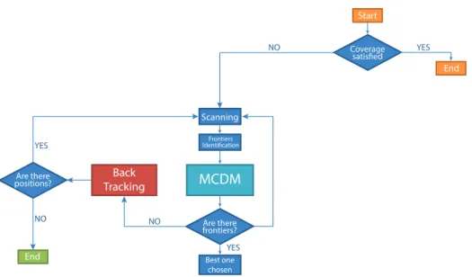
As shown in Chapter 2, the Next-Best-View approach consists in the repe-tition of different steps until a chosen condition is satisfied, usually the full coverage of an environment’s map. Often these steps are the following: ac-quire and integrate a scan from the current position, identify the next best position to reach, reach it, acquire and integrate the new scan in the global map representing the phenomenon that the robot is perceiving. Following an approach like this, it could happen that the robot goes into a corridor and then it is not able to move anymore since it does not see any further interesting position in front of it. For this reason, in the online exploration field the adoption of backtracking techniques allowing the robot to go back to previous pose until it can find a new unexplored path to follow is largely diffused. These basic concepts are collected and modeled in Figure 4.1, that summarizes how the Next-Best-Smell algorithm works.

Looking at the flowchart and starting from the top, the first operation we do at every iteration of the algorithm is to check if we have reached the coverage target we chose before. There are no limits in it; in our tests we were able to cover the full map but it is also possible to adopt a coverage value less than 100%. If this condition is satisfied, the algorithm ends with success otherwise a control loop starts.

(40)

Back Tracking Scanning End End Start Best one chosen Frontiers Identification Are there frontiers? Coverage satisfied Are there positions? MCDM NO NO _NO YES YES YES

Figure 4.1: After checking the termination condition, the robot scans the surround-ing environment, identifies new candidate positions and, after havsurround-ing evaluated them, selects the best one. These steps are iterated untill the full coverage is reached.

This loop represents the core of our online approach and it is repeated until the coverage constraint is fullfilled or the robot comes back to the initial position without other candidate poses.

The first operation performed by the robot is a scanning of the sur-rounding environment, with the limitation introduced by the Field of Vision parameter adopted. The scanning phase consist in marking as seen, assign-ing a value of 2, those cells visible from the robot’s current position. If it can find, with the method that will be shown in the following section, po-sitions candidate to be reached on the edges separating the known and the unknown area, it can start the evaluation phase.

Evaluating a position consists in applying the Choquet Fuzzy Integral described in Chapter 3, to get a score belonging to [ 0, 1] . All those positions from which the robot can’t acquire a new portion of the map are discarded; the others are collected in a record with their evaluation. If there is at least one frontier in this record, the best one (the one with the highest score) is chosen as the next goal position. Therefore the robot will reach it and it will redo all the previous steps, starting from the evaluation of the coverage condition, until the algorithm’s end.

If there are no interesting frontiers, it means that the robot is stuck at the end of a corridor or it has already explored all the cells around it. At this point it performs a backtracking operation: the robot returns to its

(41)

Back Tracking Information Gain Sensing Time Travel Distance A* Ray Casting MCDM

Figure 4.2: The three criteria are calculated with different techniques: ray casting is used to estimate the value of information gain and sensing time, while A* is implemented for the travel distance.

previous pose or, if it can’t find any further candidate position from there, to the last pose that allows it to find a new path to follow. While perform-ing backtrackperform-ing, if the robot comes back to the initial position it means that there are no more candidate positions in the map and therefore the exploration ends, in most of the case successfully (as it will be shown in Chapter 5, in some circumstances the robot could not complete the full map coverage, even if the number of ignored cells is almost irrelevant compared to the total one).

4.2 Techniques used for Implementation

In this section we describe the techniques adopted to calculate the three criteria used in the evaluation phase: information gain, sensing time and

travel distance. In the end it will be also explained how the exploration

phase is implemented in the algorithm.

Figure 5.1 represents the flowchart of our algorithm with the evaluation block expanded. As it is possible to see, the evaluation phase is computed using the Multi Decision Criteria Making approach that merges the three criteria’s contribution in a single utility function, as described in Chapter 2.

(42)

Listing 4.1: Ray caster pseudocode

1 robotX , robotY := c o o r d i n a t e s of the robot in the map

2 _{x , y := c o o r d i n a t e s of cell to scan}

3 _{curX , curY := robotX , robotY} _{// c u r r e n t cell of the ray}

4 _{m := 0} _{// v a r i a b l e to move along the ray}

5 _{hit := 0} _{// set to 1 if an o b s t a c l e is hit by the ray}

6 slope := atan2 ( y - robotY , x - robotX ) // slope b e t w e e n the cell to

7 _{// scan and the robot}

8 _{if ( d i s t a n c e from robot to cell to scan <= range )} _{// ray is cast only}

9 _{// if the cell is in}

range

10 while ( hit == 0) // move along the ray until o b s t a c l e is found

11 _{curX = robotX - m * sin ( slope )} _{// get c o o r d i n a t e s of c u r r e n t}

12 _{// cell of the ray}

13 curY = robotY + m * cos ( slope )

14 _{if ( o b s t a c l e in curX , curY ) hit = 1} _{// if cell c o n t a i n s an}

15 _{// obstacle , stop the ray}

16 _{if ( curX == x && curY == y )} _{// if the ray r e a c h e s the cell}

17 _{cell is v i s i b l e} _{// to scan , then it is v i s i b l e}

18 stop ray // stop the ray when cell is found

19 _{else m = m + 0.2} _{// move along the ray until o b s t a c l e}

20 _{// is found or cell to scan is r e a c h e d}

4.2.1 Ray Casting

In order to implement the criteria of information gain and sensing time, we implemented a ray caster.

Ray casting is a rendering technique first introduced by Arthur Appel

in 1968, and has been used for a variety of tasks in the computer graphics field.

The basic idea behind ray casting is to find what is to trace various rays from the eye, one for each pixel, and then find the closes object that blocks the path of that ray.

Our ray caster works in the following way: given a cell of interest, which in the case of calculating the value of information gain for a candidate po-sition would be a free cell which has not yet been scanned, the slope of the line connecting the centers of the cell of interest with the one of the current position is calculated.

If the line lies inside of the FoV of the robot, and the distance between the center of the considered cell and the current robot position is not greater than the range of the TDLAS sensor, a ray is shot along the line.

By moving along the ray in small increments, each cell traversed by the ray is analyzed: if an obstacle is found, the ray is stopped, otherwise if the ray reaches the cell of interest it means that it is visible from the current

(43)

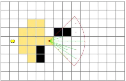
Figure 4.3: Ray casting used to calculate the value of information gain of a candidate pose. When a ray reaches the center of a free cell, the information gain value is increased.

position. An example of a ray being casted in pseudocode is shown in 4.1. In Figure 4.3 we can see rays being casted to calculate the information gain of a candidate pose. The centers of visible cells are reached by rays, while rays pointed at non visible cells are blocked by obstacles.

The value of information gain is calculated as the number of free cells which have not yet been scanned and are visible from the candidate pose (Figure 4.4).

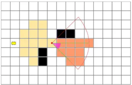
The value of sensing time is calculated as the angle between the first and the last rays to be shot in order to scan all the free unscanned cells visible from the candidate pose, and the values of the two slopes are stored to define the angle used in the following sensing operation (Figure 4.5).

Other than for these two criteria, we also used ray casting to identify candidate positions at each step of the algorithm, by finding visible free cells which are on the boundary between scanned and unscanned area.

4.2.2 A*

The last criteria we have to address is the travel distance, computed as the distance between the robot’s current position and the target one. To have an estimate as precise as possible of such distance, we implemeted the A*

(44)

Figure 4.4: The information gain of a candidate pose is the number of visible free unscanned cells.

Figure 4.5: The sensing time of a candidate pose is the angle between the first and last rays shot to scan all the free unscanned cells visible from that pose.

(45)

algorithm, developed by Peter Hart et al. [19] as extension of Dijkstra work [13].

A* uses a best-first search to find the minimum cost path from an ini-tial node to one goal node. Best-first search is a search algorithm which explores a graph by expanding the most promising node chosen according to a specified rule. Traversing the graph, A* builds up a tree of partial paths; the leaves of this tree (called the open set or fringe) are stored in a queue ordered by a cost function combining a heuristic estimate of the cost to reach a goal and the distance traveled from the initial node. Specifically, the cost function is

f(n) = g(n) + h(n). (4.1)

where g(n) is the cost of getting from the initial node to n and h(n) is a heuristic estimate of the cost to get from n to any goal node.

To find the shortest path, the heuristic function must be admissible, meaning that it never overestimates the cost to get to the closest goal node from the actual one. In our experiments we use both the Euclidean distance and the Manhattan one.

If the heuristic h satisfies the additional condition h(x) ≤ d(x, y) + h(y) for every edge (x, y) of the graph (where d denotes the length of that edge), then h is called consistent. In this case, A∗ can be implemented more ef-ficiently, no node needs to be processed more than once. A pseudocode example of how A∗ works is provided in the following Listing 4.2.

We provide a little example to clarify the operation perfomed by this algorithm largely used for plath planning purpose. In Figure 4.6 a robot and the target cell to reach are represented in a grid map. As first step, A* assigns a different value to each possible cell the robot can reach from its current one: in the example, a value of 10 is assigned to orthogonal cells, while a value of 14 to those diagonals. These value are reported in black in the image, and they represent the cost g(n) to move from the actual position to that cell.

The red number represents instead the estimated distance between the con-sidered cell and the goal, according to the heuristic chosen h(n), in this case the Manhattan distance. This is calculated as the length of the path between two points in a grid based on a only horizontal and/or vertical movements (that is, along the grid lines).

The second step computed by A* is to sum g(n) and h(n) for all the cells and select the one with the smallest value. Starting from this point, the first step is repeated, expanding in the search tree the node corresponding to the

(46)

Listing 4.2: A* pseudocode

1 f u n c t i o n A *( start , goal )

2 _{c l o s e d s e t := the empty set} _{// The set of nodes a l r e a d y}

e v a l u a t e d .

3 _{o p e n s e t := { start }} _{// The set of t e n t a t i v e nodes to be}

evaluated ,

4 i n i t i a l l y c o n t a i n i n g the start node

5 _{c a m e _ f r o m := the empty map} _{// The map of n a v i g a t e d nodes .}

6

7 _{g _ s c o r e := map with d e f a u l t value of I n f i n i t y}

8 _{g _ s c o r e [ start ] := 0} _{// Cost from start along best known path .}

9 // E s t i m a t e d total cost from start to goal t h r o u g h y .

10 _{f _ s c o r e = map with d e f a u l t value of I n f i n i t y}

11 _{f _ s c o r e [ start ] := g _ s c o r e [ start ] + h e u r i s t i c _ c o s t _ e s t i m a t e ( start ,}

goal )

12

13 _{while o p e n s e t is not empty}

14 _{c u r r e n t := the node in o p e n s e t having the lowest f _ s c o r e []}

value

15 if c u r r e n t = goal

16 _{return r e c o n s t r u c t _ p a t h ( came_from , goal )}

17 18 _{remove c u r r e n t from o p e n s e t} 19 _{add c u r r e n t to c l o s e d s e t} 20 for each n e i g h b o r in n e i g h b o r _ n o d e s ( c u r r e n t ) 21 _{if n e i g h b o r in c l o s e d s e t} 22 _{c o n t i n u e} 23 24 _{t e n t a t i v e _ g _ s c o r e := g _ s c o r e [ c u r r e n t ] + d i s t _ b e t w e e n (} current , n e i g h b o r ) 25 26 _{if n e i g h b o r not in o p e n s e t or t e n t a t i v e _ g _ s c o r e < g _ s c o r e [} n e i g h b o r ] 27 _{c a m e _ f r o m [ n e i g h b o r ] := c u r r e n t} 28 _{g _ s c o r e [ n e i g h b o r ] := t e n t a t i v e _ g _ s c o r e} 29 _{f _ s c o r e [ n e i g h b o r ] := g _ s c o r e [ n e i g h b o r ] +} h e u r i s t i c _ c o s t _ e s t i m a t e ( neighbor , goal ) 30 if n e i g h b o r not in o p e n s e t 31 _{add n e i g h b o r to o p e n s e t} 32 33 return f a i l u r e 34 35 _{f u n c t i o n r e c o n s t r u c t _ p a t h ( came_from , c u r r e n t )} 36 _{t o t a l _ p a t h := [ c u r r e n t ]} 37 _{while c u r r e n t in c a m e _ f r o m :} 38 c u r r e n t := c a m e _ f r o m [ c u r r e n t ] 39 _{t o t a l _ p a t h . append ( c u r r e n t )} 40 _{return t o t a l _ p a t h}

(47)

Figure 4.6: The initial pose of the robot and the target cells. Different weights are assigned to orthogonal and diagonal cells.

cell having the smallest f (n), as defined in Equation 4.1, until reaching the goal. The final situation is represented in Figure 4.7.

At this point, proceeding backward from the goal to the initial pose of the robot, the path connecting these two points is built as the one passing each time in the cell minimizing Equation 4.1.

In this way, as shown in Figure 4.8, it is always possible to find the short-est path between the robot and the candidate position considered, obtaining a really good estimation of the real distance between these two points.

4.2.3 Depth-First Search

After having illustrated how we calculate information gain, sensing time and travel distance, it is also important to explain how we model and realize the online navigation. As explained in the previous section, the main problem that can arise when the robot does not follow precomputed paths is that it can be stuck at the end of a corridor or in a portion of map in which it cannot identify any further interesting position to reach. For this reason, implementing a backtracking technique that allows the robot to come back to previous positions is a good idea.

As it can be seen in Figure 4.9, we address this problem modeling the exploration as a search problem solved using the Depth-First Search (DFS) algorithm with backtracking, investigated for the first time by Charles Pierre Tr´emaux in the 19th century.

(48)

Figure 4.7: The cumulative costs are spread from the starting point to the goal one, expainding always in the tree the node with the smallest value.

Figure 4.8: The shortest path is found proceeding backwards from the goal and selecting each time the cell with the minimum f (n) value.

(49)

Depth first search with BT Back Tracking Information Gain Sensing Time Travel Distance A* Ray Casting MCDM

Figure 4.9: The backtracking operations is performed modeling a search problem with a depth-first search algorithm.

Differently from most cases that use DFS to explore a graph, we have not a preassigned graph containing the poses of the robot; every time the robot reaches a new one, we add it in the tree structure adopted as a leaf of the parent node representing the previous pose of the robot. Moreover, the new position is added to a closed list to prevent the robot to reach it another time in the future. In correspondence of each pose we also save all the other frontiers identified by the robot with it. The structure we obtain is represented in Figure 4.10.

The exploration phase takes place in this way: as said, we build a tree in depth adding each time the new pose as a child of the previous one; to each node is associated a list called nearCandidate of frontiers visible from that pose. This list, initially empty, is filled every time the robot reaches a new position with those frontiers that provide new information about the map. When the robot can not find further position in front of it, it evaluates all those frontiers inside the nearCandidate record. After having possibly reached all of them and followed new paths, it performs a backtracking operation to the upper level of the tree. These steps, reported in Figure 4.11, are repeated until the coverage is obtained or the robot reaches the initial pose without completing the task.

If we image the environment map as a graph in which each free cell is a node, the only possibility to not explore entirely this graph is that it’s not

connected. In graph theory, an undirected graph is called connected when

there is a path between every pair of vertices. In a connected graph, there are no unreachable vertices.

Given this definition it is obvious that it is impossible to fully explore a map 29

(50)

Figure 4.10: Structure of the tree built during the navigation. Every time the robot reach a new position, this is add in the free with a list of all frontiers visible from there

only if there are some free and unreachable cells, maybe because the access to them is prevented by the ostacles. This is true both in simulation and in the real scenario.

4.3 ROS Implementation

We implemented the Next-Best-Smell algorithm on the Robot Operating

Sys-tem (ROS) platform [2] to run it on the robot platform used during our tests.

In this section we provide only a brief overview of the system, please refer to Appendix A for full details.

The peculiarity of ROS is that every communication between two nodes is realized with an asynchronous system based on the publish − subscribe paradigm. However, if needed it, there is also the possibility to use syn-chronous calls (through the service oriented system).

Our algorithm, implemented in the mcdm framework node, subscribes to

move base/global costmap/costmap topic as shown in Listing 4.3, provided

by the map base node, to get the costmap 2d of the environment in which the robot is located. A costmap is a map in which the obstacles are inflated by a user defined radius. For our navigation purposes, this fact prevents to choose as goal a pose too close to walls or obstacles, in a way the robot can’t reach it due to its kinematics or physical constraints.

After the Next-Best-Smell algorithm identifies a new pose, a

Move-BaseGoal message is created and sent to move base node (Listing 4.4). This

(51)

1°

3°

4° 5°

2°

Figure 4.11: Every time the robot can not find any further frontiers in front of it, it comes back to the previous pose and try to expand the corresponding node towards a new direction

Listing 4.3: Subscription ot map server node to the the global costmap of the environ-ment 1 _{if ( m a p _ s e r v i c e _ c l i e n t _ . call ( s r v _ m a p ) ) {} 2 3 _{c o s t m a p _ s u b = nh . subscribe < n a v _ m s g s :: O c c u p a n c y G r i d >( " m o v e _ b a s e} / g l o b a l _ c o s t m a p / c o s t m a p " , 100 , g r i d _ c a l l b a c k ) ; 4 _{c o s t m a p _ u p d a t e _ s u b = nh . subscribe < m a p _ m s g s ::} O c c u p a n c y G r i d U p d a t e >( " m o v e _ b a s e / g l o b a l _ c o s t m a p / c o s t m a p _ u p d a t e s " , 10 , u p d a t e _ c a l l b a c k ) ; 5 6 _{if ( c o s t m a p R e c e i v e d == 0) {} 7 R O S _ I N F O _ S T R E A M ( " w a i t i n g for c o s t m a p " << std :: endl ) ; 8 _} 9 10 _{if ( c o s t m a p R e c e i v e d == 1) {}

11 _{// all the code is inside this block}

12 } 13 14 _{sleep (1) ;} 15 _{ros :: s p i n O n c e () ;} 16 _{r . sleep () ;} 17 18 _} 31

(52)

Listing 4.4: Sensing a MoveBaseGoal message to move the robot to the next pose 1 m o v e _ b a s e _ m s g s :: M o v e B a s e G o a l goal ;

2 _{double o r i e n t Z = ( double ) ( target . g e t O r i e n t a t i o n () * PI / ( 2 * 1 8 0 ) ) ;}

3 _{double o r i e n t W =} _{( double ) ( target . g e t O r i e n t a t i o n () * PI /(2 * 180) ) ;}

4 _{move ( p . point . x ,p . point .y , sin ( o r i e n t Z ) , cos ( o r i e n t W ) ) ;} 5

6 // -7

8 _{void move ( int x , int y , double orZ , double orW ) {}

9 _{m o v e _ b a s e _ m s g s :: M o v e B a s e G o a l goal ;} 10

11 M o v e B a s e C l i e n t ac ( " m o v e _ b a s e " , true ) ; 12 _{goal . t a r g e t _ p o s e . header . f r a m e _ i d = " map " ;}

13 _{goal . t a r g e t _ p o s e . header . stamp = ros :: Time :: now () ;}

14

15 _{goal . t a r g e t _ p o s e . pose . p o s i t i o n . x = x ;} 16 _{goal . t a r g e t _ p o s e . pose . p o s i t i o n . y = y ;} 17 _{goal . t a r g e t _ p o s e . pose . o r i e n t a t i o n . z = orZ ;} 18 _{goal . t a r g e t _ p o s e . pose . o r i e n t a t i o n . w = orW ;} 19

20 _{R O S _ I N F O ( " S e n d i n g goal " ) ;}

21 _{ac . s e n d G o a l ( goal ) ;}

22

23 _{ac . w a i t F o r R e s u l t () ;} _{// the e x e c u t i o n flow is s t o p p e d until when}

the robot r e a c h e s the new pose

24

25 _{if ( ac . g e t S t a t e () == a c t i o n l i b :: S i m p l e C l i e n t G o a l S t a t e :: S U C C E E D E D )}

26 R O S _ I N F O ( " I ’m moving ... " ) ;

27 _else

28 _{R O S _ I N F O ( " The base failed to move " ) ;}

29 _}

in the world, will attempt to reach it with a mobile base. The move base node links together a global and local planner to accomplish its global nav-igation task.

When the robot reaches a new pose in the map, the next step is per-forming a scanning operation. Listings 4.5 and 4.6 show a parallel blocking thread that subscribes to the /ptu control/state topic to get the actual po-sition of the TDLAS gas sensor and then invokes the /ptu control/sweep service to perform the sweep.

(53)

Listing 4.5: Retrieving the exact pose of the pan-tilt unit before performing a scanning operation

1 _{void s c a n n i n g () {}

2 ros :: N o d e H a n d l e nh ( " ~ " ) ;

3 _{ros :: S u b s c r i b e r p t u _ s u b ;}

4 _{p t u _ s u b = nh . subscribe < s t d _ m s g s :: Int16 >( " / p t u _ c o n t r o l / state " ,100 ,}

s t a t e C a l l b a c k ) ;

5 _{ros :: A s y n c S p i n n e r s p i n n e r (0) ;}

6 _{s p i n n e r . start () ;}

7 _{auto start = chrono :: h i g h _ r e s o l u t i o n _ c l o c k :: now () ;}

8 _{g a s D e t e c t i o n () ;} _{// call the proper method to p e r f o r m a}

s c a n n i n g o p e r a t i o n

9 _{while ( ros :: ok () ) {}

10

11 while ( s t a t u s P T U !=3) { // check if the s c a n n i n g o p e r a t i o n has

s t a r t e d 12 sleep (1) ; 13 _{// R O S _ I N F O (" PTU status is ...% d " , s t a t u s P T U ) ;} 14 _} 15 R O S _ I N F O ( " S c a n n i n g s t a r t e d ! " ) ; 16 _{ros :: W a l l D u r a t i o n (5) . sleep () ;}

17 _{while ( s t a t u s P T U !=0) {} _{// check if the s c a n n i n g o p e r a t i o n is}

still r u n n i n g 18 _{sleep (1) ;} 19 // R O S _ I N F O (" PTU status is ...% d " , s t a t u s P T U ) ; 20 _} 21 22 R O S _ I N F O ( " Gas d e t e c t i o n C O M P L E T E D ! " ) ;

23 _{auto end = chrono :: h i g h _ r e s o l u t i o n _ c l o c k :: now () ;}

24 _{double t m p S c a n n i n g = chrono :: duration < double , milli >( end - start}

) . count () ; 25 _{t i m e O f S c a n n i n g = t i m e O f S c a n n i n g + t m p S c a n n i n g ;} 26 s p i n n e r . stop () ; 27 _{break ;} 28 _} 29 30 _} 33

(54)

Listing 4.6: Sending the right parameter to ptu control node to perform a scanning operation 1 _{void g a s D e t e c t i o n () {} 2 3 _{ros :: N o d e H a n d l e n ;} 4 _{ros :: S e r v i c e C l i e n t c l i e n t 1 = n . s e r v i c e C l i e n t < p t u _ c o n t r o l ::} commandSweep >( " / p t u _ c o n t r o l / sweep " ) ; 5 _{p t u _ c o n t r o l :: c o m m a n d S w e e p s r v S w e e p ;} 6 7 _{if ( m i n _ p a n _ a n g l e > m a x _ p a n _ a n g l e ) {} 8 _{double tmp = m i n _ p a n _ a n g l e ;} 9 m i n _ p a n _ a n g l e = m a x _ p a n _ a n g l e ; 10 _{m a x _ p a n _ a n g l e = tmp ;} 11 } 12 13 _{s r v S w e e p . r e q u e s t . m i n _ p a n} _{= m i n _ p a n _ a n g l e ;} 14 s r v S w e e p . r e q u e s t . m a x _ p a n = m a x _ p a n _ a n g l e ; 15 _{s r v S w e e p . r e q u e s t . m i n _ t i l t} _{= t i l t _ a n g l e ;} 16 _{s r v S w e e p . r e q u e s t . m a x _ t i l t} _{= t i l t _ a n g l e ;} 17 _{s r v S w e e p . r e q u e s t . n_pan} _{= n u m _ p a n _ s w e e p s ;} 18 _{s r v S w e e p . r e q u e s t . n_tilt} _{= n u m _ t i l t _ s w e e p s ;} 19 s r v S w e e p . r e q u e s t . s a m p _ d e l a y = s a m p l e _ d e l a y ; 20 21 _{if ( c l i e n t 1 . call ( s r v S w e e p ) ) {} 22 R O S _ I N F O ( " Gas d e t e c t i o n in p r o g r e s s ... <%.2 f ~%.2 f ,%.2 f > " , m i n _ p a n _ a n g l e , m a x _ p a n _ a n g l e , t i l t _ a n g l e ) ; 23 _{} else {} 24 _{R O S _ E R R O R ( " Failed to i n i t i a l i z e gas s c a n n i n g . " ) ;} 25 _} 26 27 _}

(55)

Chapter 5

Experimental evaluation

In this chapter we describe the results we obtained in simulation and in the real world, testing the Nexy-Best-Smell approach on the Husky A200 plat-form. In the end we will make a comparison with the work developed by Asif Arain et al. [6]. To do so, we will introduce first of all the parameters required by our algorithm and the evaluation metrics that measure the total execution time. Moreover we will investigate and explain how the final out-come may vary according to different values of the parameters introduced.

5.1 Parameters and Evaluation Metrics

In this section we will explain which parameters we consider during the modeling of exploration’s problem.

As introduced in Chapter 3, we represent the environment as an occu-pancy grid after having discretized the map with different resolutions. Each cell in this representation can assume three values according to its status: 0 if the cell is free and unscanned, 1 if it is occupied by an obstacle or 2 if it is free and already scanned by the robot. During the exploration, the robot uses two different grids: one, more coarse, is used for navigation purposes, to avoid situations in which the robot could crash against a wall or an obstacle; another one, finer, is used for keeping track of gas (mark cells as scanned). For this reason the first parameter is the resolution of the navigation map: in our tests we decided to use square cells with side of one meter, but it’s possible to use also the same resolution of the scanning map, that usually is higher (20 or 50 centimeters per side).

The second parameter we consider in our work is the range r of the gas sensor, used for scanning purpose. The sensor is able to scan visible cells whose center’s distance from the robot is not larger than this value. In our

(56)

experiments, depending on the map used, r assumed a value of 10 or 15 meters.

Another important parameter related to the platform used is the maxi-mum scan angle phi, already introduced in Chapter 3. As expressed before, the scan angle phi defines the sweep that the gas sensor has to perform. Due to the physical limitations introduced by the pan-tilt unit mounted on, the maximum value of this parameter is 180 degrees on the platform used for tests in the real world.

On the environment represented as a grid, the robot can assume a finite number of orientations, either 4 or 8 in our tests, depending if we con-sider only the main ones (North, East, South and West) or also the derived one (North-East, North-West, South-West and South-East). Usually having more orientations in which a scanning operation can be performed is an ad-vantage for the robot but experiments in simulation demonstrated that this is not always true in the case of greedy algorithms. As it will be explained in subsection 5.4, introducing more orentations means allowing the presence of two or more candidate positions with the same evaluation score. Therefore, from the robot’s point of view they can lead to similar path even if they can evolve in complete different ways due to the presence of obstacles in the map. Because our algorithm is based on the Next-Best-View concept, we cannot establish which is the best position (among the ones with the same rank) minimizing the exploration time, and therefore it is impossible to solve this conflict without negating the hypothesis of the greedy approach.

The last parameter the user can set is the threshold value used during the pruning operation. As mentioned in Chapter 4, we model the entire exploration as a search problem, building a tree in which each node is a pose of the robot and whose children are the possible poses reachable from the parent node. In this scenario, a threshold helps the robot to speed up the navigation towards the more interesting poses, whose evaluation score is greater than the pruning value, and discarding the others.

The main feature we analyzed is the total exploration time, that is esti-mated as the sum of the travel time and the sensing time. While in simula-tion it is only an estimate of the real one, for experiments in the real world the total exploration time is computed starting from the instant in which the ROS node of the algorithm is launched and ending when the exploration is completed, either successfully or not. Since the exploration time is affected by many factors it was our interest to discover which ones they are and track how they influence it.

The first and most important evaluation metric is represented by the total number of sensing positions, or how many times the robot stops to

(57)

perform a sensing operation in order to detect the presence of gas. Directly connected to this, the travel distance, computed with A*, is an estimation of the real path followed by the robot and connecting all the sensing posi-tions starting from its initial pose to the last one. Given that and assuming the robot is moving with costant speed of 0.5 m/s it is easy to compute an approximation of the time spent traveling.

As said before, every time time the robot stops it performs a sensing operation and thanks to ray casting, as described previously in Chapter 4, we are able to compute the exact angle required to observe the unscanned area. The sum of all these angles represents another evaluation metric, used to estimate the total scanning time with a polynomial function.

5.1.1 Criteria Weights

As described in Chapter 3, we modeled the decision related to the next position to reach as a multi-objective optimization problem, in which we considered three criteria: information gain, travel distance and sensing time. The advantage of using the Choquet Fuzzy Integral instead of a different aggregation function is the possibility to model relationships among coalition of the criteria considered. Taking inspiration from Game Theory, we can define a coalition as any subset of criteria. Therefore it is clear that, trying to optimize three criteria and three coalitions among them means solving a 6-dimensional problem.

The goal of our simulated experiments was to identify a set of weights that could guarantee good results in terms of total exploration time. To make it easier we reduced our problem to three dimensions, focusing our attention only to the three single criteria and modeling a slighty synergic relationship among them. In this way we were able to represent this problem in a graphical way: due to the following constrains

x₁+ x2+ x3= 1 (5.1)

and considering x1 ≥ 0, x2 ≥ 0, x3 ≥ 0 we can draw a simplex as space of

the solutions.

Trying to solve this problem didn’t represent a good idea since it is only a rough approximation, without considering the coalitions of more than one criterion, of the real 6-dimensional problem. Therefore we ran a large number of tests, under different conditions and using different maps, and we analized the results obtained.

First of all we identified some points of interest on the simplex surface and we tested their performance. These points are the following ones: the