Alma Mater Studiorum · Universit`
a di Bologna
Scuola di Scienze Corso di Laurea in Fisica
Performance studies of the CMS
distributed analysis system in the associated
Higgs boson production with top quarks
Relatore:
Prof. Daniele Bonacorsi
Correlatori:
Prof. Andrea Castro
Dott. Giuseppe Codispoti
Presentata da:
Giovanni Tenaglia
Sessione II
3
Sommario
L’obiettivo di questa tesi `e studiare la fattibilit`a dello studio della produzione associata t¯tH del bosone di Higgs con due quark top nell’esperimento CMS, e valutare le funzionalit`a e le caratteristiche della prossima generazione di toolkit per l’analisi distribuita a CMS (CRAB versione 3) per effettuare tale analisi.
Nel settore della fisica del quark top, la produzione t¯tH `e particolarmente interessante, soprattutto perch`e rappresenta l’unica opportunit`a di studiare direttamente il vertice t-H senza dover fare assunzioni riguardanti possibili contributi dalla fisica oltre il Modello Standard. La preparazione per questa analisi `e cruciale in questo momento, prima dell’inizio del Run-2 dell’LHC nel 2015. Per essere preparati a tale studio, le implicazioni tecniche di effet-tuare un’analisi completa in un ambito di calcolo distribuito come la Grid non dovrebbero essere sottovalutate. Per questo motivo, vengono presenta-ti e discussi un’analisi dello stesso strumento CRAB3 (disponibile adesso in versione di pre-produzione) e un confronto diretto di prestazioni con CRAB2. Saranno raccolti e documentati inoltre suggerimenti e consigli per un team di analisi che sar`a eventualmente coinvolto in questo studio.
Nel Capitolo 1 `e introdotta la fisica delle alte energie a LHC nell’esperimento CMS. Il Capitolo 2 discute il modello di calcolo di CMS e il sistema di analisi distribuita della Grid. Nel Capitolo 3 viene brevemente presentata la fisica del quark top e del bosone di Higgs. Il Capitolo 4 `e dedicato alla preparazione dell’analisi dal punto di vista degli strumenti della Grid (CRAB3 vs CRAB2). Nel capitolo 5 `e presentato e discusso uno studio di fattibilit`a per un’analisi del canale t¯tH in termini di efficienza di selezione.
5
Abstract
The goal of this work it to investigate the feasibility of the study of the asso-ciated t¯tH Higgs boson production with top quarks in the CMS experiment, and to evaluate the functionalities and features of the next-generation CMS distributed analysis toolkit (CRAB version 3) to perform such analysis. In the top physics sector, the t¯tH production is particularly interesting, mainly because it represents the only opportunity to directly probe the t-H vertex without making assumptions about possible contributions from sources beyond the Standard Model. The preparation for this analysis is crucial now, before the LHC Run-2 starts in 2015. In order to be prepared for this study, the technical implications of running a full analysis in a Grid-aware distributed computing environment should not be underestimated. For this purpose, an investigation of the CRAB3 tool itself (available now in pre-production mode) and a direct performance comparison with CRAB2 is presented and discussed. Suggestions and advices to the analysis team that will eventually be involved in this study are collected and documented. In Chapter 1 the High-Energy Physics at the LHC in the CMS experiment is introduced. Chapter 2 discusses the CMS Computing Model and the Grid distributed analysis system. In Chapter 3 the top quark and Higgs boson physics are briefly presented. Chapter 4 is dedicated to the preparation of the analysis from the point of view of the Grid tools (CRAB3 versus CRAB2). In Chapter 5 a feasibility study of a t¯tH analysis in terms of selection efficiency is presented and discussed.
Contents
1 High-Energy Physics at the LHC in the CMS experiment 1
1.1 The LHC accelerator at CERN . . . 1
1.2 The experiments at the LHC . . . 2
1.2.1 ALICE, ATLAS, CMS, LHCb . . . 2
1.2.2 The CMS detector . . . 4
1.3 Run-1 experience and preparations for Run-2 . . . 7
2 The CMS Computing Model and the Grid distributed anal-ysis system 9 2.1 The Worldwide LHC Computing Grid (WLCG) . . . 9
2.2 The CMS Computing Model . . . 10
2.3 Distributed GRID analysis with CRAB2 in Run-1 . . . 11
2.4 Evolving to CRAB3 for Run-2 . . . 13
3 Top quark and Higgs boson physics 15 3.1 Steps in the discovery of the top quark and the Higgs boson . 15 3.1.1 Role of the Higgs boson in the Standard Model . . . . 18
3.2 Properties and phenomenology . . . 19
3.3 t¯tH production . . . 21
4 Preparing a t¯tH analysis with CRAB3 25 4.1 Introduction . . . 25
4.2 Testing CRAB3 versus CRAB2 . . . 26
4.2.1 Tests with Workflow A . . . 27
4.2.2 Tests with Workflow B . . . 30
4.2.3 Tests with Workflow C . . . 31
4.2.4 Summary of tests outcome . . . 32
4.3 Comparing CRAB3 and CRAB2 on a real analysis task . . . . 36 i
5 A real example: t¯tH analysis 41
5.1 Trigger . . . 41
5.2 Kinematic selection . . . 41
5.3 b-tag . . . 42
5.4 t¯t system reconstruction and kinematic fit . . . 43
5.5 Higgs boson’s mass . . . 44
Chapter 1
High-Energy Physics at the
LHC in the CMS experiment
1.1
The LHC accelerator at CERN
The Large Hadron Collider (LHC) [1] is a particle accelerator, currently the largest in the world, based at CERN laboratories near Geneva, between Switzerland and France. Its purpose is to help finding an answer to the main issues of particle and theoretical physics, such as the exact differences between matter and antimatter, the consistency of the Standard Model at very high energies, the nature of dark matter and energy, the existence of extra dimensions, the origin of mass or the reason of the symmetry breaking in the electro-weak force. For the last two items, the search for the Higgs boson could provide a clue.
The LHC is a 27 Km underground hollow ring where two opposite beams of protons or ions, travelling into separate pipes, are forced to collide in four points where the detectors of the four experiments (ALICE, ATLAS, CMS and LHCb) are located. A section of the ring can be seen in Figure 1.1. The pipes are kept at ultrahigh vacuum to avoid collisions with air or gas particles. In order to force the particles to circulate inside the circuit, LHC is endowed with electromagnets cooled with superfluid helium at temperatures below 2K, making the Niobium-Titanium cables become superconductive and able to produce a strong magnetic field of above 8T.
The LHC is supplied with protons obtained from hydrogen atoms inside the linear accelerator Linac 2 or lead positive ions produced by another linear accelerator, Linac 3. Linear accelerators use radiofrequency cavities to charge cylindrical conductors. The ions pass through the conductors, which are alternately charged positive or negative. The conductors behind them push
Figure 1.1: Section of the collider ring.
particles and the conductors ahead of them pull, causing the particles to accelerate. During acceleration, electrons (eventually all) are stripped away by an electric field. Even here, magnets ensure that the particles follow the circuit.
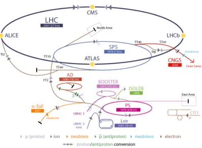
These two machines are only the beginning of the injection chain ending in the main ring: Linacs - Proton Synchrotron Booster (PSB) - Proton Synchrotron (PS) - Super Proton Synchrotron (SPS) - LHC, as shown in Figure 1.2. At each step of the chain the energy of the particles is increased, allowing them to reach the final energy of currently about 4 TeV. The external accelerators of the chain are designed to meet the strict LHC requirement of 2808 high intensity proton bunches in the ring.
1.2
The experiments at the LHC
The detectors sitting in the four experiment chambers are an essential part of the LHC project.
1.2.1
ALICE, ATLAS, CMS, LHCb
• ALICE (A Large Ion Collider Experiment) is a detector dedicated mainly to heavy ion (Pb) collisions and searches for the formation of quark-gluon plasma, a state of matter thought to be the one formed fractions of second after the Big Bang. For this reason, this state
3
Figure 1.2: The CERN accelerators complex, including the production chain.
needs extreme conditions to be created: hadrons should “melt” and the quarks should free themselves from their gluonic bonds. Finding this plasma and testing its properties should contribute to verify and improve the current quantum chromodynamics (QCD) theory, maybe clarifying the reason of the confinement phenomenon observed inside hadrons.
• LHCb (Large Hadron Collider beauty) investigates the differences be-tween matter and antimatter by studying the bottom quark, also called “beauty” quark. The peculiarity of this experiment is that to catch the b quarks, among all the variety of quarks produced, movable tracking detectors close to the path of the beams circulating in the pipes have been developed, instead of surrounding the entire collision point.
• ATLAS (A Toroidal LHC ApparatuS) and CMS (Compact Muon Solenoid), conversely, are more general-purpose experiments; in fact they “simply” analize data resulting from collisions of various kinds through the char-acterization of the debris passing through a set of subdetectors that surround the collision point. The CMS detector is described in more detail later on in this chapter, while the approach adopted to select only the relevant data within the enormous amount of data flowing from the detector during LHC operations will be described in section 5.1.
The last but not the least important aspect of the LHC project is the way in which recorded data (almost 30 Petabytes annually) are processed and stored. This is performed through the WLCG, the Worldwide LHC Computing Grid, a global computer network of over 170 computing centres, located in 34 countries, mainly in Europe and in the United States. After the filtering, an average of 300Mb/s of data flow from CERN to large computing centres on high-performance network connections, including both private fiber optic cable links - the “LHC Optical Private Network” (LHC-OPN) - and existing high-speed portions of the public Internet.
1.2.2
The CMS detector
Figure 1.3: The CMS detector.
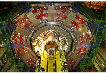
The Compact Muon Solenoid (CMS) detector[2] is installed along the path of the LHC collider ring, in French territory. It is composed by five cylindrical layers, as can be seen in Figure 1.3, and in Figure 1.4 with more detail.
At the heart of the structure, near to the pipes, lays the tracker, whose task is to track the charged particles produced in every collision. The tracker is composed of a pixel detector with three barrel layers, closest to the colli-sion point, and a silicon micro-strip tracker with 10 barrel detection layers. Here also the decays of very short-living particles (like bottom quarks) can be seen. The core part of the pixels and the micro-strips is essentially a recti-fying junction that is activated by the passing of a charged particle. Tracker components are so dense that each measurement, accurate to about 10 µm, can resolve the trajectories even from the collision with more debris.
5
Figure 1.4: A scheme of the CMS structure.
The second layer is the electromagnetic calorimeter (ECAL), used to record the energy of photons and electrons. This task is performed by mea-suring the light, proportional to the particle energy, produced by the scintil-lation of lead tungstate (PbWO4) crystals. The light detection is carried by avalanche photodiodes.
The third layer is the hadronic calorimeter (HCAL). It is important for the measurement of hadronic “jets”, the stream of particles originating from the decay of a hadron, and indirectly neutrinos or exotic particles resulting in missing transverse energy. Other two calorimeters are placed outside the calorimeter to complement its action for lower angles of production and out-side the solenoid to stop the hadrons that pass through the main calorimeter. Also these calorimeters are based on a scintillation measurement technique, but need different reactive materials: plastic scintillators (quartz fibres in the forward detector, more fitting for the higher energies of the low angle debris) and hybrid photodiodes for the final readout.
The fourth layer is the solenoidal magnet giving the name to the entire machine. In fact it is fundamental to distinguish different charged particles by allowing the determination of the charge/mass ratio, bending their trajectory with a different curvature radius with its magnetic field.
The fifth layer is composed by the muon detectors that, as the name sug-gests, identify muon tracks, measure their energy and also collect informa-tions for data filtering. These tasks need three types of detectors: drift tubes (DT), cathode strip chambers (CSC) and resistive plate chambers (RPC). The first ones are concentrated in the central “barrel” region. They contain stretched positively-charged wires within a gas, and work as tracking
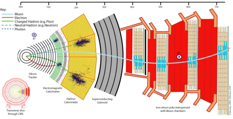
detec-tors collecting the electrons produced in the gas by the ionising particles. The second ones are placed in the endcap region, and provide pattern recognition for rejection of non-muonic backgrounds and matching of hits to those in other stations and to the CMS inner tracker. CSC’s are similar to DT’s but in addition they have negative charged (cathode) strips to collect positive ions from the gas. Strips and wires are perpendicular, so they provide a bidi-mensional position information. The third ones consist of two parallel plates, one positively-charged and another negatively-charged, both made of a very high resistivity plastic material. They collect the electrons and ions produced in the gas layer separating them. These electrons in turn hit other atoms causing an avalanche. The electrons resulting are then picked up by external metallic strips, to give a quick measurement of the muon momentum, which is then used by the trigger to make immediate decisions as of whether the data are worth keeping. This is necessary in order to avoid useless data to be stored, wasting data storage space and time. In this layer, moreover, a steel yoke of multiple layers confines the magnetic field of the solenoid and hosts the return field. The joint operation of all the components described above enables the CMS detector to provide a full reconstruction of the events, as shown in Figure 1.5.
Like CMS, ATLAS is a multi-purpose apparatus, designed to examine a
Figure 1.5: The products of a collision event as reconstructed by detectors. variety of different kind of collisions, and it has many similar concepts ap-plied, but there are differences, e.g. the resolution that can be obtained in several measurements or the available range of the measurements, due
7 to different design choices. ATLAS uses a 2T magnetic field, surrounding only the tracker, that yields lower resolution but less structural restrictions. Moreover, the use of different active materials make ATLAS have a better resolution on the HCAL-based measurements but worst on the ECAL side.
1.3
1 experience and preparations for
Run-2
Now, LHC is near the end of a period of shutdown which began on February 14, 2013, to perform maintenance operations and to prepare the machine for a higher energy and “luminosity” when reactivated in early 2015 for the second data taking period, or “Run-2”. For example, about 10000 superconducting magnet interconnections have been consolidated, and this year the Super Proton Synchrotron (SPS) has been powered up to provide higher energy particles. The final collision energy of the next data taking period should be of about 14TeV, almost the double of the maximum reached so far. This will increase the discovery potential, allowing further studies on the Higgs boson and potentially enabling to shed light on the dark matter mystery or find supersymmetric particles.
This year a further analysis of data collected during “Run-1” brought more evidence about the existence and the consistency with the Standard Model of the Higgs boson. Conversely, recent studies seem to be in contrast with the supersimmetry theory.
An improvement of the CMS and ATLAS experiments intrumentation and triggering system is planned for the next years.
Proposals have been put forward for a “High Luminosity” LHC, an upgrade possibly starting in 2018. They are included in the “European Strategy” plan aiming to make the machine capable of collecting ten times more data by around 2030. The future steps of this plan will depend on the results of the next runs, but there are some ideas about a “High Energy” LHC upgrade and even a “Very High Energy” upgrade that may comprehend the construction of a new collider ring 80 to 100 km long [3].
Chapter 2
The CMS Computing Model
and the Grid distributed
analysis system
2.1
The Worldwide LHC Computing Grid
(WLCG)
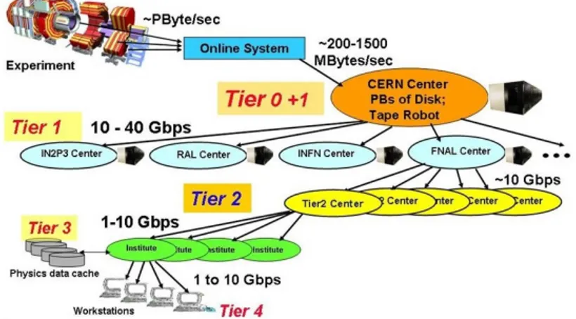
Figure 2.1: Scheme of the GRID hierarchy of computing units. In order to handle the enormous amount of data flowing from the de-tectors, the LHC experiments have equipped themselves with sophisticated online trigger systems to select only the data relevant for their physics pro-gram, as well as complex offline infrastructures, capable of storing the LHC data and offering also the computing power to process the data for anal-ysis purposes. Due to the stringent constraints driven by the challenging
LHC operating parameters, the LHC experiments adopted computing sys-tems based on Grid technologies. The Worldwide LHC Computing Grid is the collaboration that orchestrates all this for the 4 LHC experiments. The building block of such systems are the middleware components developed by projects like EGI in Europe and OSG in the United States; on top of these, each experiment equipped itself with a Computing model that exploits both the common infrastructure and the common services to fulfil the needs of the experiments. In the following, a brief description of the types and roles of the computing centres for CMS is provided.
The CERN computer centre, considered the zero level, or “Tier-0”, of the Grid, has dedicated 10 Gbit/s connections to the counting room. Other data are sent out from CERN to the “Tier-1” centres, that is the first level of the external computing resources, 13 important academic Institutions in Europe, Asia, and North America, via dedicated 10 Gbit/s links, the “LHC Optical Private Network”. These institutions receive specific subsets of the RAW data, for which they serve as a custodial repository for CERN, and also perform reprocessing when necessary. The “Tier-2” centers, typically located at universities and other scientific Institutes that can store sufficient data volumes, are connected to the “Tier-1” centres, transferring data from/to them. The Tier-2s constitute the level dedicated to Monte Carlo simulation and data analysis. Continuing in a branch-like structure, we find the “Tier-3” centres, small computing sites with no obligations towards WLCG which are mainly devoted to data analysis.
2.2
The CMS Computing Model
The CMS data acquisition system collects and processes the information from all the detectors at every collision “event”, that is at the LHC frequency of 40 MHz. Thanks to a trigger system, events are filtered and selected, and the rate of events recorded for offline processing and analysis is of the order of a few hundreds of Hzs. The amount of data collected is still considerable, so all the analyses must be done offline, not only while the machines are running, and for this purpose a lot of storage space is needed. This need can be addressed by relying upon the already mentioned WLCG project.
The CMS offline computing system supports the storage, transfer and ma-nipulation of the recorded data. In addition, it supports production and distribution of simulated data, as well as access to conditions and calibration information and other non-event data. It accepts real-time detector infor-mation from the data acquisition system at the experimental site; ensures
11 conservation of the data for successive re-usages; supports additional event filtering or data reduction for more specific purposes; in synthesis, it supports all the physics-driven computing activities of the entire collaboration. Data regarding collision events that pass the trigger are physically stored, includ-ing provenance informations, as persistent ROOT files, that is files accessible with ROOT, a data analysis framework developed at CERN, object oriented in its design to easily deal with the many different kinds of information con-tained in each event.
In order to maintain a certain level of flexibility, CMS makes use of several event formats for these files:
• RAW events contain the full recorded information from the detector, plus a record of the trigger decision and other metadata;
• RECO (reconstructed data) are produced by applying several levels of pattern recognition and compression algorithms to the RAW data; • AOD (Analysis Object Data) is the compact analysis format,
contain-ing all data regardcontain-ing high-level physics objects;
• Other non-event data required to interpret and reconstruct the events. The data collections, sorted by physics meaningful criteria, are called “datasets” in the CMS jargon: each dataset physically consists of a set of ROOT files, each with a physical names, and the mapping from the logical names and the physical file names is maintained in multi-tiered cataloguing systems. Processing and analysis of data at sites is typically performed by the user submission of “jobs”, such as personalized data processing or Monte Carlo simulations generation, on available computing resources in remote sites via the Grid middleware services. On top of such services, CMS uses its official and very popular tool for distributed analysis, which is called CRAB (CMS Remote Analysis Builder).
2.3
Distributed GRID analysis with CRAB2
in Run-1
CRAB is a tool developed within the CMS workload management develop-ment team to open Grid resources to any member of the CMS Collaboration. It aims to give to any CMS analysts access to all the data recorded and pro-duced by the experiment, in a way they are accessible via uniform interfaces regardless of where they are physically located on the WLCG infrastructure.
CRAB was designed to hide as much as possible the Grid complexities from the end-users, so to maximise the analysis effectiveness.
The core goal of CRAB is to prepare and execute the user’s analysis code on the available remote resources, and exploit them as much as possible as if the user would execute his/her task interactively on a loc[al machine. In a nutshell, CRAB has to collect the user’s analysis code and prepare it to be shipped to the worker node (WN) on the computing farm of the site that will be selected for processing the user task; discover the location(s) on the WLCG of the input dataset requested by the user, split the user task into jobs according to the specification by the user, and rely on the Grid Information system (and other mechanisms) to decide where to actually send each of the jobs; submit the jobs to the selected remote resource, where the analysis code will open and read the dataset requested as input; provide all status information as frequently as asked by the user; at the end of the processing, collect the final output of the processing plus all the log files, which may be useful to debug failures and/or to get information on the analysis task just completed, job per job, in full details.
During LHC Run-1, all analyses have been performed with the version 2 of the CRAB toolkit, called CRAB2 [4] in the CMS jargon. For a CRAB2 user, the standard actions to be performed in an analysis submissions and monitoring were:
• crab -create: to collect the user code, package it, find the input datasets location and perform job splitting
• crab -submit: to submit the jobs to the Grid
• crab -status: to gather status information about the submitted jobs • crab -getoutput: to retrieve the user output
The CRAB toolkit has been in production (and in routine use) by end-users since 2004, despite its usage increased considerably with the start of LHC Run-1. During this operational experience, the CRAB2 server ran as a 24x7 service and successfully managed all the requested user workflows. Since 2010, the number of distinct CMS users running analysis every day using CRAB2 averaged about 250 individuals, reaching peaks of more than 350 distinct users per day. Looking at the number of jobs submitted in the last years, since 2010 an average of approximately 200k distinct jobs per day were submitted to perform CMS data analysis, and were successfully managed by CRAB2 [5].
Before Run-1 started, focussed computing challenges showed that, on a statis-tics of a total of 20 million analysis jobs submitted between 2008 and 2009,
13 the total success rate of CRAB2 jobs is 64.1%, with a 9.4% of failures re-lated to Grid middleware issues in general, but the largest fraction of failures (23.3%) had to be addressed to non-Grid problems, like application-specific issues or site issues [6].
The fraction of successful CRAB2 jobs varies depending on the type of sub-mitted workflow: it can be as high as > 85% for jobs accessing Monte Carlo simulations, but for jobs accessing data it averages approximately 75%[7].
2.4
Evolving to CRAB3 for Run-2
Despite the large success of CRAB2 for the CMS experiment, including being used for the discovery of a particle whose characteristics are compatible with the Higgs boson, the CMS Computing developers team studied the Run-1 ex-perience in details and agreed that there are motivation for evolving CRAB2 further. A complete discussion on the technical motivation for such choice are beyond the scope of this thesis, and they are just briefly summarised as follows. The CRAB2 client-server model has demonstrated to improve the management of analysis workflows, and its logic should be kept. The sim-plification of the user experience through the handling of most of the jobs load out of his hands and “behind the Grid scenes” is a value that should be kept in any future design, and possibly improved further. Ultimately, the optimisation of the resource usage, by exploiting at its best the modern Grid middleware from very few central points (servers) allows to improve the overall scalability of the whole system.
The CMS Computing developers have been working on first versions of a CRAB3 system [8]. This has been ready and open for beta-testing during some part of the Summer 2014, and it was possible to exploit this golden chance and try the tool out in this work since the early phases of its wide deployment. The results in chapter 4 are based on using the latest CRAB3 release, in order to gain familiarity with the tool and to try to prepare a ttH analysis in the future of the CMS distributed computing environment. Some CRAB3 characteristics can be easily seen when trying to use the tool for real analysis operations. One specific feature is summarised in the following. A full report on the experience collected in using CRAB3 is reported in Chapter 4.
CRAB3, unlike CRAB2, automatically tries to resubmit failed jobs, in order to free the users from the concern of checking every time how many jobs have effectively succeeded. However, some disadvantages of this new feature could be that the completion time now becomes more difficult to estimate or that users will hardlier notice a recurring problem, such as a crashed
site, if the system automatically bypasses it, and it can even resubmit the failed job on the very same site. They become more “blind” regarding the software operations, but this could be an advantage for physicists, who can thus concentrate more on their research task, and maybe are less used to face this kind of issues.
Chapter 3
Top quark and Higgs boson
physics
3.1
Steps in the discovery of the top quark
and the Higgs boson
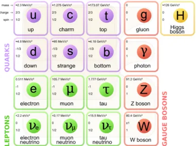
Figure 3.1: The particles of the Standard Model.
The top quark is one of the fundamental particles in the Standard Model, represented in Figure 3.1 [9]. Its existence had been theorized since the discovery in 1977 of the bottom quark by the Fermilab E288 experiment team. This is because quarks, particles having spin 12, result to be naturally
divided into “generations”, couples of two quarks with respectively −1 3 and 2
3 in electron’s electric charge units. For this reason the newly-discovered
quark, with charge −13e, seemed to strongly call for the existence of another quark with charge 2
3e. In analogy with the other two generations, this quark
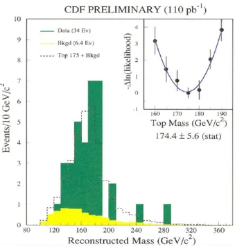
was expected to be heavier than the bottom quark, requiring more energy to be created in particle collisions, but not by much. However, early searches for the top quark at SLAC and DESY experiments, using a new kind of proton-antiproton colliders, gave no result. Then, the Super Proton Synchrotron at CERN and the Tevatron at Fermilab started a real “race” for the discovery of the missing particle. But when SPS reached its energy limits the top quark did not make an apparition yet, establishing the inferior limit for its mass at 77 GeV/c2. Z and W bosons were instead found, and researchers understood that at high energies the products of a collision tend to decay into “jets” of numerous less energetic particles. So the right jets could represent a trace of the top quark generation, therefore a new detector relying on their detection, DØ, was added to the Tevatron complex, in addition to the Collider Detector at Fermilab (CDF). At those times the Tevatron was the most powerful collider in the world, so it represented the best hope for this search. In 1993 the mass inferior limit was pushed to 131GeV/c2, and finally, on April 22, 1994, the CDF group found 12 candidate events that seemed to indicate the presence of a top quark with a mass of about 175 GeV/c2, as
shown in Figure 3.2. In the meantime, also the DØ group, analysing past data, found some evidence. A year later on March 2, 1995, after further analyses and reanalyses, the two groups jointly reported the discovery of the top quark with two compatible values for the mass: 176±13 GeV/c2 by CDF and 199±30 GeV/c2 by DØ[10].
But the research was all but finished, even though all the quarks seemed to have been discovered. The serious problem was that all the most ac-cepted theories solving the unification of weak and electromagnetic force predicted even the massive particles to be massless. Following early works by Y. Nambu, J. Goldstone, P. Anderson and J.S. Schwinger, a possible so-lution emerged in 1964 with works by R. Brout, F. Englert, P. Higgs, G. Guralnik, C. Hagen and T. Kibble.[11] The key was the introduction of the so-called “Higgs field”, whose quantum is the “Higgs boson”, that could ex-plain the electroweak symmetry breaking. In 1967 this theory was included in the first formulation of the Standard Model because calculations consis-tently were able to give answers and predictions, but there was no experimen-tal proof. After the discovery of the top quark, proving the existence of the Higgs ”mechanism” finding the Higgs boson became the central problem in experimental physics. The first attempt was done with the Large Electron-Positron Collider (LEP) at CERN, even if it had not been designed for this
17
Figure 3.2: The first measurement of the top quark mass.
purpose, in 1986. But at the end of the run, in 2000, the evidence for the production of a Higgs boson was insufficient to justify another run, and LEP was dismantled to make room for the new LHC. These results, however, set a lower bound of the Higgs boson’s mass at 114.4 GeV/c2 due to the energy limits of the machine. In addition some processes probably involving this particle in its virtual form were observed.
The following research was carried out by the newly upgraded Tevatron proton-antiproton (p¯p) collider at Fermilab, but even there the boson wasn’t observed, fixing tighter limitations on its possible characteristics. In 2009 LHC started its activity and two years later both CMS and ATLAS experi-ments independently reported a possible excess of events at about 125 GeV. So the search was focused around that energy value. On July 31, 2012, the ATLAS collaboration improved the significance of the finding of a new parti-cle, having a mass of 126±0.8 GeV/c2, to 5.9 standard deviations. CMS also
improved the significance to 5 standard deviations with the particle’s mass at 125.3±0.9 GeV/c2. These data were compatible, so researchers needed only the confirmation that this particle was the one searched for. Finally, on March 14, 2013, CERN confirmed that it was precisely the Higgs bo-son, after having verified its predicted properties, and having measured more accurately its mass, as shown in Fig. 3.3.
Figure 3.3: One of the most precise measurements of the Higgs boson mass.
3.1.1
Role of the Higgs boson in the Standard Model
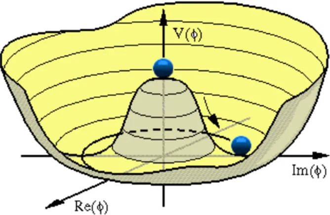
It has been experimentally observed that only fermions whose spin is in the opposite direction of its motion can interact electroweakly, and not their “mirror versions”, as could be expected. In other words, some of these pro-cesses are possible but their mirror images are not, so it is said that elec-troweak interactions break the “chiral symmetry”. But the lagrangian equa-tion of a particle must satisfy, according to quantum chromodynamics and electrodynamics, the gauge invariance of the group SU(3) x SU(2) x U(1). These two conditions impose the vanishing of the lagrangian term contain-ing the mass, so all the particles result to be massless. The solution of this problem is a scalar complex field H with a potential shaped as a “mexican hat”, as pictured in Figure 3.4, as it maintains a symmetrical structure, but for which the stable states lying in the lowest potential region, where the field reaches its “vacuum expectation value”, are asymmetrical. Because the value of the potential at H = 0 must be 0, the vacuum expectation value is v, different from 0, and this suggest that the field equation can be written as h(φ) = v + H(φ), where v is a constant. Moreover it can be shown that its lagrangian equation (more precisely the lagrangian density) is
L = −∂µh∗∂µh + m2h∗h − λ(h∗h)2− λfhf∗f − g2W+W−h2− ρ2(Z0)2h2
where λ is the auto-interaction “coupling constant” (a measure of the proba-bility of an interaction event), f is the wave function of any fermion, m is the
19
Figure 3.4: The Higgs field potential V , in function of the complex phase φ of the Higgs field.
mass of the Higgs boson and λf are its coupling constant respectively with
the Higgs field, with the W boson and with the Z0 boson. This coupling has
thus the term λfvf∗f , that can be schematized as a Feynman diagram with
only two vertices (see Figure 3.5) and λfv as the coupling constant. This
process can occur at every time and has no products but the fermion itself, and the rate of its continuous occurrence (λfv) represents the mass of the
fermion. It can be seen from the equation that this happens also for W and Z
Figure 3.5: Feynman diagram of an interaction of a fermion with the Higgs field.
bosons and for the field itself, giving also the Higgs boson a mass. The other vertices predicted by the lagrangian equation represent the interaction of the considered particles with the Higgs boson. This generation of the property “mass” is called the “Higgs mechanism”.
3.2
Properties and phenomenology
The mass of the Higgs boson, according to the last measurements by CMS and ATLAS experiments, is 125.03±0.41 GeV/c2 (CMS) and 125.36±0.55
GeV/c2 (ATLAS)[12]. It has also been confirmed that the Higgs boson has no electric or color charge, its spin is 0 and its parity is +1 (the processes in
which it is involved do not break the chiral symmetry). It has a mean lifetime of 1.56 × 10⁻²² s, then it decays in many possible ways, called “channels”, having different probabilities, called “branching ratios”, to occur. Branching
Figure 3.6: Plot of the branching ratios of the Higgs boson’s decay. They have been determined using the programs HDECAY and Prophecy4f, based on the Standard Model [13].
ratios (see Figure 3.6) change dramatically across the possible range of the Higgs mass making it necessary to take into account different strategies for the Higgs identification depending on its mass. The most probable decay of a Higgs boson with the recently measured mass turns out to be into a couple of bottom and antibottom quarks, with a branching ratio of almost 60%. As the products are quarks, they actually cannot continue to exist in free form because of the “quark confinement”. That forces part of their energy to transform into gluons, which in turn decay into couple of a quark and an antiquark. These can release other energy generating other quarks or bind together forming hadrons, that may split again if the energy of their constituents is high enough. These cone-shaped “showers” of hadrons are called “jets” and can be reconstructed by detectors of the ATLAS and CMS experiments, allowing to trace the original products with appropriate algo-rithms.
A Higgs boson can be produced at LHC much like other particles through different processes (see Figure 3.7), the dominant one being the gluon-gluon fusion, with a “cross section” of between 20 and 60 pb. The cross section is a quantification of collision probability; it is measured in barn (b), equivalent
21
Figure 3.7: Plot of the production cross sections of the Higgs boson at an energy of 8 TeV.
to 10−24 cm2, and represents the interaction probability per unit flux. In
fact, the event rate can be obtained multiplying the cross section by the instantaneous luminosity. The production through the W vector boson fusion qq→qqH (10% of the gg→H cross section) is also frequent.
3.3
t¯
tH production
In this analysis, events consistent with the production of a top-antitop quark pair in association with a Higgs boson will be selected, where the top-antitop quark pair decays into a bottom-antibottom quark pair and other two couples of quarks from the decays of two W bosons, and the Higgs boson decays to a bottom-antibottom pair of quarks, generating a total of 8 jets. This channel, as it can be seen in Figure 3.8, is not one of the likeliest, having a cross section of about 0.13 pb at 8 TeV, a factor 100 smaller than the dominant gluon-fusion pp→H production. But an observation with this signature would be interesting for a number of reasons. The rate of this process depends on the couplings of the Higgs boson to the top quark and the bottom quark. These are key couplings that must be measured in order to establish consistency with the predictions of the Standard Model. Because of the large mass of the top quark the value of its coupling constant with the Higgs boson is very
Figure 3.8: Some of the Higgs boson production modes. It is important to notice that the Higgs boson is not the only product of many of these processes.
high (almost 1 according to Yukawa theory).
It appears that t¯tH production represents the only opportunity to directly probe the t-H vertex without making assumptions about possible contribu-tions from sources beyond the Standard Model. In fact, since the Higgs boson mass results to be smaller that the top quark mass, decays of the Higgs boson producing a top quark do not occur, and the measurement of Standard Model cross sections depending on top quarks becomes the only way to estimate the intensity of the coupling. One of these cross section concerns the gluon fusion diagram, pictured above, in which a fermion loop (more likely a top quark loop) produces the Higgs boson. This mechanism, as seen in the previous section, dominates the Higgs boson production, but the constraining of the top quark Yukawa coupling relies on the assumption that particles not predicted by the Standard Model do not contribute to the loop diagram. So, a direct probing of the coupling can be made instead by looking at the pp→t¯tH process.
The reason of the top quark’s heaviness itself can be an interesting object of research. Moreover, t+H is also present as final decay state of many new physics scenarios (such as “little Higgs”, “composite Higgs”, extra di-mensions...), the validity of which could be hinted by the observation of a significant deviation of the measured rate of t¯tH production with respect to predictions.
With respect to the bottom quark, there are several other processes that can be used to probe its coupling with the Higgs boson, typically the associated production involving either a W or Z boson (VH production). The t¯tH sig-nature however yields a probe that is complementary to the VH channel,
23 with t¯t+jets instead of W+jets providing the dominant background contri-bution. In fact, the couple bottom quark/W boson is the almost exclusive product of the decay of the top quark, so the final state t¯tH is characterized by the way the two W boson decay. Here the so-called “all-hadronic” case will be considered, in which the two W bosons both decay into quarks (in turn hadronizing all into jets), since it is the most likely, covering almost 50% of the cases, while the remaining fraction is associated to the so-called “single-lepton” or “double-lepton” channels. The final products depend also on the way the H decays, and for this the H→b¯b decay, that has the highest branching ratio, will be considered here.
A negative aspect of the analysis on this channel is the strong presence of QCD backgrounds. They can be however reduced by the request for events having a certain number of jets recognized (see section 5.3) as originated by a bottom quark, the so called “b-tagged” jets, in the event. In this analysis a request of 4 such jets will be applied.
Chapter 4
Preparing a t¯
tH analysis with
CRAB3
4.1
Introduction
As outlined in Chapter 2, a CMS analysis user submits jobs to the Grid using the CRAB toolkit. In the CMS analysis operations during Run-1, the CRAB2 version of the tool was used, while currently the CMS Computing developers are working on the next generation of the tool, known as CRAB3. As this thesis investigates an analysis effort that may become concrete in the future, and helps in preparing this analysis also from the technical point of view, it is worthwhile to investigate how easy/difficult (or just different) it would be to run such analysis in the CRAB3 environment. For this purpose, in the scope of the current thesis, the new features of CRAB3 were tested as a beta-tester. In fact, it was possible to profit of a very fruitful testing period in Summer 2014 in which the CMS Computing project was involved in a Computing, Software and Analysis challenge (CSA 2014). This CMS activity also involved massive tests of CRAB3 as a pre-production system, and this thesis contributed as well. In addition to this, some job submissions needed for this thesis and performed with CRAB2 were also tried out with CRAB3. The final goal is to offer to future analysis users some directives and suggestions not only on the physics side, but also on the computing tools side. While a real data analysis is discussed in Chapter 5, the current Chapter focusses on preparing such analysis with CRAB3.
4.2
Testing CRAB3 versus CRAB2
The CRAB3 tool has been designed and developed to prepare and submit bunches of CMS analysis jobs on the WLCG Tier-2 level. This task was and still is performed also by CRAB2, but CRAB3 improves several features and fixes some issues that were found using CRAB2 during Run-1. As a common point, both CRAB2 and CRAB3 create, submit and monitor jobs until completion, but in general CRAB3 is designed to be more easy to use and to hide even more complexity to the users, in order to offer a more satisfactory analysis experience to the end users.
This chapter presents the work done to familiarise with CRAB3 and its main features, the CRAB3 versus CRAB2 comparison based on selected perfor-mance figures, and a description of the analysis environment adequate in CRAB3 for a t¯tH analysis in the future.
To achieve this, we prepared and submitted specific workflows which have been found relevant to test CRAB3. As it was done in CRAB2, these will be referred to as “tasks”, thus following the CRAB jargon. The following is an introduction and definition of the workflows adopted and submitted to the Grid with CRAB3:
• a Monte Carlo generation workflow, which uses CRAB3 to actually create simulated events samples for analysis purposes. These tasks will be limited in size to 100 jobs per task. In the following, this workflow will be referred to as “Workflow A”.
• a Monte Carlo generation workflow like the aforementioned one, but whose tasks are not limited to 100 jobs per task but can be composed by one thousands of jobs per task (or more). In the following, this workflow will be referred to as “Workflow B”.
• an analysis workflow that accesses existing Monte Carlo simulated datasets on the Grid and perform access operations on them. This is a very common and popular use-case, of course, and also different in characteristics with respect to the previous two, hence it is quite rele-vant to add this workflow in the tests. In the following, this workflow will be referred to as “Workflow C”.
All workflows were submitted using the same version of the CRAB3 client (version 2.10.7 patch1). In total, 54 tasks of the various types have been submitted to the Grid using CRAB3: 46 of them were of the type Workflow A or Workflow B, and the remaining 10 were instead analysis tasks of the type Workflow C, addressed to a particular Monte Carlo dataset.
27 An overview of the outcome of all submissions can be found in Tables 4.1, 4.2 and 4.3. A discussion can be found in the following paragraphs, one paragraph per workflow. Before this, it is worth to describe the metrics introduced and used in the analysis. Such metrics are:
• “Requested”: this figure refers to the number of jobs that are configured to be created and submitted as from the CRAB3 configuration file itself (crab.cf g). For example, in case a task of 100 jobs is created and executed with no problem whatsoever, it would eventually end up in running exactly 100 jobs with neither failures nor resubmission. • “Submitted”: this figure refers to the total number of jobs that end up
to be eventually submitted to the Grid to finalize a task. This number is by construction equal or larger than the “Requested” number of jobs. For example, in case a task of 100 jobs is created and executed with just 1 job failure and a subsequent single resubmission which ends up suc-cessfully, this figure would eventually be equal to 101 jobs “submitted” to finish the task.
• “Delivered”: this figure reports the ratio of the actually successful jobs over the total of the requested ones. For example, whatever the number of needed resubmissions have been, if at the end a user is getting 99 jobs out of the “Requested” 100 jobs, this ratio is 99%.
• “Submission overload”: this figure is the ratio of the difference “Sub-mitted - Requested” over the total of “Requested” jobs, and it esti-mates, despite in a rough manner, the amount of additional load on the CRAB3 infrastructure caused by failures-and-retries cycles.
4.2.1
Tests with Workflow A
In the execution of Workflow A, a total of 24 tasks composed by 100 jobs each have been created, submitted to the Grid with CRAB3, monitored un-til completion, and analysed in terms of their final results. Out of these 24 tasks, 1 task was considered for exclusion from the collected statistics, as it completely failed due to known or predictable infrastructure issues (e.g. scheduled downtimes). As a result of this exclusion, the number of valid sub-missions for Workflow A resulted in a total of 23 tasks. The grand summary of the submissions for Workflow A is shown in Table 4.1 and discussed in the following.
The “Delivered” fraction of jobs per task was observed to be on average about 91% for Workflow A. A user can hence expect CRAB3 to end up in
Table 4.1: The average CRAB3 successful deliver rate and job overload per-centage for workflow A (see text for explanations).
Task Requested Submitted Delivered Submission
number [nb. jobs] [nb. jobs] [%] overload [%]
1 100 101 100.0% 1.0% 2 100 100 100.0% 0.0% 3 100 104 100.0% 4.0% 4 100 109 100.0% 9.0% 5 100 105 100.0% 5.0% 6 100 122 99.0% 22.0% 7 100 104 100.0% 4.0% 8 100 113 100.0% 13.0% 9 100 422 98.0% 322.0% 10 100 590 100.0% 490.0% 11 100 549 100.0% 449.0% 12 100 103 100.0% 3.0% 13 100 100 100.0% 0.0% 14 100 300 0.0% 200.0% 15 100 101 100.0% 1.0% 16 100 100 100.0% 0.0% 17 100 101 100.0% 1.0% 18 100 100 7.0% 0.0% 19 100 101 95.0% 1.0% 20 100 102 98.0% 2.0% 21 100 201 100.0% 101.0% 22 100 100 100.0% 0.0% 23 100 100 100.0% 0.0% Average 91.2% 70.8%
29
Table 4.2: The average CRAB3 successful deliver rate and job overload per-centage for workflow B (see text for explanations).
Task Requested Submitted Delivered Submission
number [nb. jobs] [nb. jobs] [%] overload [%]
24 1000 1157 95.5% 15.7% 25 1000 1124 99.5% 12.4% 26 1000 1111 100.0% 11.1% 27 1000 1005 99.9% 0.5% 28 1000 1000 100.0% 0.0% 29 1000 2274 88.9% 127.4% 30 1000 2056 98.0% 105.6% 31 1000 1001 100.0% 0.1% 32 1000 1001 99.9% 0.1% 33 1000 1054 99.9% 5.4% 34 2000 2388 91.4% 19.4% 35 2500 4590 91.8% 83.6% 36 1500 1563 100.0% 4.2% 37 2000 2560 99.8% 28.0% 38 3000 3242 99.8% 8.1% Average 97.6% 28.1%
Table 4.3: The average CRAB3 successful deliver rate and job overload per-centage for workflow C (see text for explanations).
Task Requested Submitted Delivered Submission
number [nb. jobs] [nb. jobs] [%] overload [%]
39 53 92 86.79% 73.58% 40 53 64 94.34% 20.75% 41 53 90 100.00% 69.81% 42 53 59 96.23% 11.32% 43 53 53 88.68% 0.00% 44 53 53 92.45% 0.00% 45 19 19 94.74% 0.00% 46 259 295 99.62% 13.46% Average 94.1% 23.6%
delivering back a very high percentage out the originally “Requested” jobs, thus demonstrating that a very good throughput is indeed offered to end-users by the CRAB3 toolkit. On the other hand, the amount of “Submission overload” that CRAB3 has to digest to achieve the aforementioned goal was found to be not negligible at all. For Workflow A, this variable was measured to be about 71%: in other words, the average number of jobs that the CRAB3 server submits to complete a task which originally comprised 100 jobs has been 165 jobs on average. This means that the jobs dealt with by CRAB3 (e.g. including resubmission of failed jobs) to satisfy the user request were almost 2/3 more than the original workload. With respect to CRAB2, these resubmissions in CRAB3 are invisible to the end user for an explicit design feature of CRAB3 versus CRAB2; on the other hand, this admittedly implies that, behind the scene, the overall Grid/CRAB system is actually automati-cally managing an overload of jobs that is hard to predict and impossible to control by the user. In a nutshell, the transparency offered by CRAB3 to the users has a value (no need for constant monitoring, no need to act to trigger resubmissions, etc), but this value comes with a cost to be paid by the infras-tructure, and this work tried to quantify it. Digging this aspect a bit further, in some cases this overload may just have been related to jobs which did fail at the Grid middleware layer(s) and hence never accessed any WNs (worker nodes) on the WLCG computing sites. But in many other cases, this may have been related to jobs that indeed ran and failed, then ran again, perhaps failing again (also repeatedly), before being actually declared as unsuccessful once and for all. The latter case, if not properly tuned, would yield a con-siderable waste of CPU time at the Tier-2 level. This could be investigated further by verifying that the applied CRAB3 server logic guarantees that the CPU waste at the T2 level stays to a minimum level. Investigating this would require to access and study e.g. logs from specific machines running CRAB3/gWMS services, which goes beyond the scope of the current work. On the other hand, in the scope of this thesis this “Submission overload” observable was measured also for the other workflows (see next paragraphs). It emerges that this investigation is promising and would require additional focussed work, with a deep involvement of the CRAB3 development team.
4.2.2
Tests with Workflow B
In the execution of Workflow B, a total of 20 tasks have been created, submit-ted and monitored until completion. These 20 tasks can be divided into two sets: 14 tasks made of 1000 jobs each, and 6 tasks made of more than 1000 jobs each (ranging from 1500 to 3000 jobs). Out of these 20 tasks, 5 were considered for exclusion for known or predictable infrastructure issues (e.g.
31 scheduled downtimes), hence the number of valid submissions for Workflow B corresponds to a total of 15 tasks. The grand summary of the submissions for Workflow B is shown in Table 4.2 and discussed in the following.
The “Delivered” fraction of jobs per task is on average about 98% for Work-flow B, i.e. even higher than WorkWork-flow A. This is an indication of an excellent performance of the CRAB3 tool on larger tasks. The amount of “Submission overload” that CRAB3 has to digest to achieve this was found to be much smaller for Workflow B than for Workflow A, i.e. about 28%. In other words, the “Submission overload” in case of Workflow A and B was roughly 2/3 and almost 1/3 more than the original submitted workload, respectively. The smaller overload in case of Workflow B may be somehow related to the bene-fit of creating and submitting larger tasks with CRAB3 on the Grid: having to deal with 1000-jobs (or more) tasks versus 100-jobs tasks may reduce the actual amount of interactions with several system components, thus reducing the chances that an error condition or a service failure may occur. This is discussed more at the end of this chapter, especially in connection with the analysis of the job failure modes.
4.2.3
Tests with Workflow C
In the execution of Workflow C, a total of 10 tasks have been created, sub-mitted and monitored until completion. Among these 10 tasks, 8 tasks are made of 53 jobs, one is made of 19 jobs and another one is made of 259 jobs. It was arranged like this to emulate possible configurations of analysis users accessing a standard, a less-than-standard and a more-than-standard amount of simulated events inside a very popular CMS dataset on the Grid. Out of these 10 tasks, 2 were excluded for known or predictable infrastructure is-sues (e.g. scheduled downtimes), hence the number of valid submissions for Workflow C actually corresponds to a total of 8 tasks. The grand summary of the submissions for Workflow C is shown in Table 4.3 and discussed in the following.
The “Delivered” fraction of jobs per task is on average about 94% for Work-flow C, i.e. slightly lower but still comparable to WorkWork-flow A and B. This is again a confirmation of a very good performance of the CRAB3 tool, not only on Monte Carlo generation workflows as Workflow A and B, but also on a very different (and popular) type of workflow in which a specific Monte Carlo dataset residing on a limited amount of sites is requested for access. For Workflow C, the amount of “Submission overload” that CRAB3 has to digest behind the scenes is smaller than it was for Workflow B, and much smaller than Workflow A. As a concise summary, it could be stated that the “Submission overload” for Workflow A, B, C has been measured to
be roughly 2/3, almost 1/3, about 1/4 of the original requested workload, respectively. The smallest overload observed for Workflow C may find an explanation in the fact that these jobs can run only on specific sites hosting the input datasets to the jobs, thus yielding a limited set of profitable Grid sites for such tasks: while the interactions with the system components are the same, the failure modes caused - as in Workflow A and B - by a large set of sites some of which may expose site issues, are much more limited for Workflow C. This is discussed more in the following.
4.2.4
Summary of tests outcome
As a summary of the investigations about the two main metrics discussed in the previous paragraphs, the average fraction of “Delivered” jobs and the “Submission overload” measured in the tests performed for Workflow A, B and C are shown in Figure 4.1.
Figure 4.1: Representation of the percentages of delivered jobs and submis-sion overload for Workflow A, B and C
In addition, it is interesting to investigate the error types observed for failed jobs in all the submissions. The data are taken from the Dashboard [14], and the breakdown into failure modes is shown in both Table 4.4 and Figure 4.2. They will be briefly discussed in the following.
33
Table 4.4: Breakdown into failure modes for jobs of all workflows submitted to the Grid.
Workflow Total success Failures [%] Monitoring
rate [%] Grid Application Site glitch [%]
A 76.0 12.4 0.1 0.2 11.3
B 82.3 13.9 0.4 1.0 2.4
C 63.7 4.5 2.1 6.0 23.7
The first metric a submitter is interested to look at is the fraction of successful jobs over the total amount of submitted jobs. By “successful”, here, it is meant a job which eventually ends with a “0 exit status”, i.e. no error. Over the submissions performed, about 76% and 82% of the jobs corresponding to Workflow A and B have finished successfully, while this percentage is about 64% for Workflow C (see Table 4.4). The success rates for Workflows A and B can be considered relatively good (and compatible with each other, within the available statistics). The success rate for Workflow C is instead not as good. It is not possible to explain the reason for these figures only from the average numbers quoted above: a look into specific information on the outcome of the jobs belonging to the submitted tasks forming each of the Workflow can cast some light, though. This further check was performed, with a data-mining on the submission statistics in details. It was observed that the failure rates for Workflows A and B are mostly due to individual tasks which ended up as complete failures at submission time, due e.g. to unpredictable infrastructure problems (it should be remembered that CRAB3 is roughly beta-installation at the time of these tests, so not a production-quality infrastructure for CMS yet). In terms of frequency of this error condition, it was found that this happened to a minority of the tasks, roughly less than 15-20%: despite not low, for a real user the problem may cause a relatively low damage, and may be solved by a CRAB3 automatic resubmission of all jobs within a task which failed in its entirety. The situation is different for the lower success rate of Workflow C: it may be explained by the fact that this kind of task needs to run only on the sites hosting the input dataset and requiring this data to be served efficiently, i.e. being more exposed to failures on this small pool of sites (e.g. I/O-related errors). Another observation is that while for the generation workflows (Workflows A and B) the failures were massively concentrated in just few tasks, for the analysis workflow (Workflow C) the failures were spread more uniformly across all tasks, yielding to a larger number of tasks not 100% completed. This may be more problematic to end users, as a full analysis may need to run on an entire dataset and not a fraction of it, and any technical obstacle to this would yield latencies, and ultimately a potential impact on the physics analysis throughput.
Concerning the breakdown into failure modes (see Table 4.4), it was ob-served that a non negligible fraction of the non-successful jobs had issues at the monitoring level, i.e. their full details could not be extracted from the Dashboard monitoring. This was particularly inconvenient, as this study relies on such monitoring platform to avoid the need to manually dig into plenty of log files. An alternative approach was evaluated, i.e. to use the glidemon infrastructure [15] as monitoring system; unfortunately, this is by
35 design a semi-realtime tool, focussed on latest monitoring data with a scarce historical depth, and somehow more oriented to service monitoring that to end-user monitoring. In a nutshell, we were left partially blind to the actual failure reasons of a non-negligible fraction of jobs, namely about 11%, 2%, 24% of the failed tasks for Workflow A, B and C respectively. Despite this undesired situation, some observations can still be done. Firstly, the impact of the aforementioned problem is negligible at least for Workflow B (only about 2% of the failure reasons were lost), so this workflow can be discussed regardless of the monitoring issue. It can be observed that the failures for Workflow B are dominated by errors at the Grid middleware level: this is always a fragile layer, especially in a pre-production system like CRAB3, and it will probably improve quickly as long as the tool (and its interactions with the middleware) matures. Concerning Workflow A and C instead, a comparative analysis is in principle not possible, but one assumption may apply here: as the glitch is affecting the monitoring layer, it may well be that the job statuses that are lost are random, i.e. all exit modes (successful or failed for any reason) are underestimated in a flat manner. If this assump-tion is reasonable, the breakdown into failures may still make sense, and provide an acceptable estimate of the sources of fragility that each workflow may encounter on a CRAB3 system. For example, a much lower number of Grid failures for Workflow C (only about 5%) may be explained by the fact that jobs are sent where the data are, i.e. in a smaller number of sites, so this submission may not be very exposed to any kind of service failure that scales as the number of involved sites. Another example is the slightly higher rate of application failures for Workflow C: this may be explained by the fact that a more complex application was indeed used for Workflow C versus Workflow A/B. A final example is the ratio of site failures: this may seem counter-intuitive, as the sites are less in number, but in this case data are heavily read in input, so Workflow C is more exposed to I/O problems. In addition it should be reminded that this work does not cover any detailed analysis on the Grid sites that ran the jobs. This would definitely be useful, as it was observed, for example, that a very recurrent error exit code was 60311, a site error indicating a stage-out failure in the job: it was possible to map a large majority of this failures to just one site, i.e. the SPRACE Tier-2 site in Brazil. Blacklisting problematic sites like this could be considered as a valid option in order to decrease the fraction of site errors.
All the observations made must be take carefully: the statistics of submis-sions is large but still this is not a scale test, and in addition a part of the analysis was affected by lack of monitoring information. Improvements in the analysis may come once more submissions will be done on a setup in which
the monitoring component will be more stable and reliable. For this purpose, this work contributed to the quality of the Dashboard software product e.g. by reporting the major observations, and also by opening official tickets to report bugs that were encountered. As an example, the lack of exposure from the Dashboard database to the Dashboard web site of some monitoring information needed for this thesis was communicated as a bug report in a ticket [16] that was quickly addressed and fixed by the developers.
Another interesting observation could be added to the list of suggestions to CRAB3 users in the future. During the execution of some of the important workflows of this work, it was realised that the choice of a default for a CRAB3 configuration parameter is definitely inadequate for the need of most CMS users (and the documentation about this is not yet updated and clear enough about it): by default, the logs of the user jobs are not saved on destination storage, unless a specific request for this is explicitly added to the CRAB3 python configuration file in the “General” section, as follows: conf ig.section (00General00)
(...)
conf ig.General.saveLogs = T rue
It must be noted that this configuration needs to be prepared before the jobs are actually created and submitted, so if a user realises this at any time after the submission of the first jobs, it is too late to roll back and the logs will not be saved. This may look like a minor detail, but it is of paramount importance for most users in their daily work: maintaining the capability to download and parse the logs by ad-hoc scripts is often the best way to assess the overall outcome of a submission or do some post-processing studies, and sometimes, e.g. in case of unreliabilities in the Dashboard monitoring, this might be also the only way to guarantee that informations about user jobs are not lost forever. It is hence strongly suggested that any CRAB3 users consider to activate this configuration flag in all the CRAB3 python configuration files in the submission preparation phase.
4.3
Comparing CRAB3 and CRAB2 on a real
analysis task
In order to get prepared to perform a complete t¯tH analysis on Grid using the next-generation of the CRAB toolkit, it was considered of importance in this thesis to prepare an additional workflow of relevance for top quark
37 physics in CMS, and submit it to Grid using both CRAB2 and CRAB3, and compare the outcome.
The workflow prepared for this study is typical in the context of a multijet analysis in the top quark physics sector. In particular, it executes two mains tasks: firstly, it skims the data from a multi-jet Monte Carlo simulated sample into a smaller fraction of events of physical interest for the study of fully hadronic top quark decays (a possible channel study for t¯tH events); secondly, it performs some internal format conversion.
The workflow was created separately in CRAB2 and CRAB3. In the first case, the “crab -create” step produced a unique task of 1271 jobs; in the sec-ond, as there is no “crab -create” step, the configuration was done by acting on the number of events per jobs inside the configuration, so to create a task which consists of the same number of jobs. This allows to directly compare e.g. the completion times per job in both cases. The jobs need to access a given dataset /T T J etsM SDecayscentralT uneZ2star8T eV − madgraph − tauola/Summer12DR53X − P U S10ST ART 53V 19 − v1/AODSIM , which, given its size (approximately 25 TB), was available in only a few Grid sites. The outcome of the submission of this real top workflow to the Grid with CRAB2 and CRAB3 are summarized in Table 4.5. It can be seen that the
Table 4.5: Summary of the results in the submission of the top physics workflow to Grid with CRAB2 and CRAB3.
CRAB Submitted Success Exit codes Average
version [nb. jobs] rate [%] for failures execution time [s] CRAB2 1269 99.5 50115 35278 50669 8021 50660 50800 50669 CRAB3 1265 99.4 137 29442 N/A N/A N/A N/A N/A N/A
success rates in the CRAB2 and CRAB3 submissions have been measured to be 99.5% and 99.4% respectively: this indicates that both systems are equally reliable and no evidence has been collected in this measurement that would suggest a user not to use CRAB3 for such kind of tasks.
It is interesting to examine the failure modes separately for the CRAB2 submission and the CRAB3 submission. It can be seen that the CRAB2 submission had 6 failures only, which are connected to a variety of causes, i.e. cmsRun not producing a valid job report at runtime (code 50115); appli-cation terminated by wrapper for undefined reason (code 50669, happening twice); FileReadError, maybe a site error (code 8021); application termi-nated by wrapper because using too much RAM, RSS (code 50660); appli-cation segfaulted (code 50800). On the other hand, it can be seen that the CRAB3 submission had 7 failures only, but the actual cause is known only for 1 of them, namely a blocked job (code 137), whereas for the remaining 6 the status of the jobs is unknown to the Dashboard (see “N/A” in Table 4.5). In a nutshell, it can be seen that CRAB2 exploits a mature and reli-able monitoring system which allows to track the real cause of error in every experienced failure, while the same maturity seems not to be available for CRAB3 submissions.
Another interesting information is the time duration of the submitted jobs in a CRAB2 or CRAB3 scenario. As shown in Table 4.5, the jobs in the CRAB2 submission last about 35k seconds on average (i.e. about 10 hours), while the jobs in the CRAB3 submission last about 29k seconds (i.e. about 8 hours). The distributions of the job duration times are also shown in Figure 4.3 and 4.4 for the CRAB2 and CRAB3 submissions respectively. The job duration are similar in both cases; actually, the jobs in the CRAB3 submission are quicker to complete, on average. This may be caused by the fact that the jobs went to better performing sites, but it could also be that the resource management in CRAB3 is more efficient than in CRAB2. We did not investigate this aspect further, though. In the scope of this thesis, it is instead of major interest the fact that it was demonstrated that a real top workflow which could run on CRAB2 so far, could also proficiently run on CRAB3. The only caution is related to the monitoring system, which needs to be strengthened and consolidated further in CRAB3 to avoid causing troubles to the end-users when monitoring and troubleshooting their jobs. Still, this study shows that a t¯tH analysis would technically be ready to be performed also in a CRAB3 environment.
39
Figure 4.3: Distribution of completion times for jobs of a real top quark workflow submitted with CRAB2.
Figure 4.4: Distribution of completion times for jobs of a real top quark workflow submitted with CRAB3.
Chapter 5
A real example: t¯
tH analysis
5.1
Trigger
The first CMS trigger that selects data to be retained or discarded is the Level 1 Trigger (L1), a hardware system which analyses particle tracks and filters only the events where some particular quantities pass a certain threshold, reducing the rate of data flow to about 100 kHz [17]. The High Level Trigger (HLT) is instead very different: it is a computer farm where a preliminar reconstruction of the events is performed, and if at least one of the trigger conditions of this level is satisfied, all the data of this event are saved and the event is classified according to the triggers passed. The HLT trigger paths can be grouped according to the topology of the event they select: “muon triggers” and “electron triggers”, for instance, select events where the HLT can identify at least one (or more) muon or electron satisfying well defined requirements; “multijet triggers” are instead characterized by high jet multiplicity. Data streams are then composed from series of events that have passed triggers which can be grouped by some feature. These only later are saved in separate datasets, where they can be accessed for various kinds of analyses. In this one data selected with only the multijet trigger (at least 4 jets with a transverse momentum ≥50 GeV) will be used. The chosen threshold on transverse momentum guarantees an acceptable trigger rate.
5.2
Kinematic selection
The final state sought after, as discussed in section 3.3, can be reconstructed from the jet variables by using a kinematic fit where the t¯t system is recon-structed first and the H→b¯b system subsequently.
Because of the choice of the all-hadronic t¯tH decay channel, a request of an 41