Automated methods in aircraft ground analyses: modelling process improvements by automated simulations

(1)

UNIVERSITA’ DI PISA

Facoltà di Ingegneria

Corso di Laurea Specialistica in Ingegneria Aerospaziale

Tesi di Laurea

Automated Methods in Aircraft Ground

Analyses: Modelling Process

Improvements by Automated Simulations

Relatori: Candidato:

Prof. Ing. Eugenio Denti Antonio Colosimo

Ing. Terence Frost Luke Bagnall

(2)

(3)

To my parents, the ones I’ve always wanted to thank, but never found the words…

(4)

Acronyms

A/C Aircraft

ACAP Airplane Characteristics for Airport Planning

ADAMS Advanced Dynamic Analysis of Mechanical Systems ADB Automated Differential Braking

ATA Air Transport Association BLG Body Landing Gear

BSCS Braking and Steering Control System BTV Brake To Vacate

CG Centre of gravity COCL Cockpit over centreline CT Cycle Time

DBD Database for design DOE Design of Experiment DOF Degree of Freedom DTS Desktop Simulation GPS Global Positioning System HCF Heading Control Function LG Landing Gears

LG-1 Landing Gear minus 1 NLG Nose Landing Gear

MAC Mean Aerodynamic Chord MLG Main Landing Gear

MRP Materials Requirements Planning MTOW Maximum Take-Off Weight

OS Oversteer

SLR Static Loaded Radius SOW Statement of Work PAX Number of passengers

TLAR Top Level Aircraft Requirements TPS Toyota Production System

(5)

TT Touch Time VSM Value Stream Map WLG Wing Landing Gear

WSCS Wheel Steering Control System XWB Extra Wide Body

(6)

Abstract

The purpose of this work is to investigate about the processes adopted to perform some Aircraft Level analyses and to create new methods and approaches in order to automate them, to speed them up, and to re-use the model created for all the aircraft.

This approach is in compliance with the principles of the Lean Philosophy developed by Toyota (based on mapping the processes, finding what is value adding, non value adding and what the sources of waste are, and trying to continuously improve the process).

The automation of the processes is based on a high level parameterisation for Groundlines and Ground Manoeuvrability analyses. The former investigates about the geometrical and mechanical static behaviour of a loaded aircraft on the ground, analysing data such as the clearances to the ground or the loads of the shock absorbers, and the parameterisation refers to all the possible positions for the Centre of Gravity (CG) and all the masses issued in the CG envelope, other than all the possible versions of the same aircraft family; the latter focuses on the dynamic behaviour of the aircraft during manoeuvres, measuring clearances to the edges of the runway, steering angle and steering torque in different conditions, and the parameterisation refers to all the possible runways the aircraft runs on, the CG position, the total mass and the position of the control point (the point on the aircraft taken as reference for controlling the aircraft).

The necessity for an automated tool arises from the limits a repetitive manual procedure have, such as the high time consumption or the possibility to make mistakes in manual data transfers.

The basis for a completely automated tool to perform all the Aircraft level analyses is described. The tool has several databases with aircraft characteristics, with the functions of the analyses and with all the possible conditions that can be encountered, and it’s not developed within this work.

The programmes the work refers to are A350XWB, A380 and the A320 family, but the methods will be applied for the same analyses on all the other aircraft.

(7)

Acknowledgements

I would like to thank Prof. Eugenio Denti and the Dipartimento di Ingegneria Aerospaziale (DIA) from Università di Pisa for having given me the opportunity to develop my thesis within my internship experience in Airbus UK.

I would like to express my sincere gratitude to Luke Bagnall for being a fantastic tutor, teaching me a lot of things and always giving me a challenging point of view in facing engineering problems.

A special thanks goes to Franco Calvanese, Leoneardo Vivarelli, Bjoern Kirchhoff and Serena Simoni for being not only fantastic colleagues, but also true friends, and for all the advice and the support they gave me.

I also wish to thank James Morris and Ryan Davies for the technical support, and Andy Bird for carefully revising part of this thesis.

A special thanks goes to Terry Frost, who always showed me silently his esteem, and drove me through difficult decisions with his advice.

I also would like to thank Luke Spencer, Simon Hancock and Steve O’ Brien.

A sincere thanks goes to my ‘mates’ Gabriele Bernardini and Cécile Garaygay, sharing with me both the life and the work experience.

A special thanks goes to my family, they have always believed in me, encouraged me and given me a helping hand in difficult moments, and they shared with me the successes as well as the delusions, making me feel the love and esteem they have for me.

(8)

Introduction

Modelling and Simulation is a branch of engineering, whose importance has highly increased over the last few years. The advantages of a model driven design are well documented, both in standard textbooks as well as engineering journals.

Through modelling, it is possible to test different solutions in a virtual way, to make modifications, to predict performances, to discover anomalies and resolve them before the real components are produced.

The Modelling and Simulation team within the Landing Gear Coc Department finds its place in this context, spreading among different design teams with the design of models to define and validate technical requirements, to the validation and verification of the landing gear system design, using a wide range of simulation techniques and analysis methods.

Among the different sections of the Modelling and Simulation team the Aircraft Level team is responsible for all aircraft modelling activities associated with the landing gear and landing gear systems, including tyres. The team provides aircraft models for two main areas, Aircraft Level Modelling and System Level Modelling. The Aircraft Level models are currently used for ground manoeuvrability with a focus on:

• Validation of Top Level Aircraft Requirements • Definition of system level requirements

• Architecture trade-off Studies

• Airport operations and compatability

As a result the main customers are, EIJ (Engineerung, Integration, J Airport Operation), Program ATA32 Integrators and chief engineers, WSCS (Wheel Steering Control System) design teams.

The System Level models are curently used for BSCS (Braking and Steering Control System) testing including:

(9)

• Steering avionic functional tests • Antiskid perfromance tests • Heading Control Function tests • Automatic Differnetial Braking Tests • AUTOBRAKE tests

• Brake to vacate tests

and are integrated onto the following test platforms:

• Desk top simulations • Landing Gear minus 1 • BSCS avionics rig • BSCS systems rig

This work is developed within the Aircraft Level team and deals with Groundlines and Ground Manoeuvrability analyses.

The approach adopted is to analyse the processes and the methods currently used within the team to perform some analyses through the production of a value stream map. Following the principles of the LEAN thinking philosophy the sources of waste are identified and reduced by proposing new techniques and methods for the building and the management of the models.

In the processes analysed in this work the greatest challenge is related with the difficulty to obtain a high level of parameterisation with the ADAMS/View tool. This requires the modeller either to build a lot of different models to run different cases or to adapt the existing models at each run, with a consistent waste of time and resources.

The purpose of the new proposed approach is to create, through a high level of parameterisation, an automated tool capable of performing at first all the cases within a single type of analysis, and then all the possible analyses the Aircraft Level team aims to perform.

The analyses taken into account for the development of this work are Groundlines, Jacking Groundlines and Ground Manoeuvrability.

(10)

The Groundlines consist in a static analysis in which a model of the Landing Gears is created, the behaviour of the shock absorbers and the tyres is modelled (with non linear spring dampers) and the aircraft is loaded with all the possible conditions (in terms of position o f the centre of gravity and total mass) provided by the CG envelope.

The aircraft is ‘dropped’ on the ground and once the steady state is reached some geometrical and mechanical data are collected, such as the closures and the loads of the shock absorbers, the pitch angle, the position of some reference points and the static deformed radius of the tyres.

Groundlines analyses are performed on the A350XWB –800/-900/-1000

The Jacking Groundlines deal with the geometrical data related to the landing gears in failure situations due to burst tyres. The condition of each tyre is modelled and all the requested cases are run to investigate about the clearances to the ground of the jacking points (the points where the lifting devices have to be mounted in order to lift the aircraft and to fix or change the wheels).

Jacking Groundlines studies are made on A380-800.

Ground Manoeuvrability analyses are made with simulations in which the aircraft is placed on a runway and through controls on the engine’s thrust and the steering angle of the nose landing gear is forced to perform the manoeuvres that occur when an aircraft is in a taxiing phase within an airport. This analysis tends to carry out the clearances to the edges of the runway while the manoeuvres take place, as well as the steering angle and steering torque applied to steer and the slip angle.

This analysis is performed on A380-800 model at first, and then through the model of a A320 is extended to all the programmes for the same purposes.

Future developments are proposed in the last chapter, in compliance with the LEAN way of thinking, pushing more towards automation and parameterisation of the processes.

(11)

Index

Acronyms……….……...i Abstract……….…...iii Acknowledgments……….…...iv Introduction………..…..v 1 LEAN Philosophy ...1 1.1 Introduction ...1 1.2 Lean history...1

1.3 The Toyota Way and the 14 Principles ...3

1.3.1 Section I: Long-Term Philosophy...4

1.3.2 Section II: The Right Process Will Produce the Right Results...4

1.3.3 Section III: Add Value to the Organization by Developing Your People 5 1.3.4 Section IV: Continuously Solving Root Problems Drives Organizational Learning...5

1.4 Specify value ...6

1.5 Value stream map...6

1.6 Improving the process ...7

2 A350XWB Groundline analysis...9

2.1 Introduction ...9

2.3 Request of work ...13

2.4 Input Data...13

2.4.1 Geometric Architecture of the gears ...13

2.4.2 CG Envelopes...14

2.4.3 Spring curves...14

(12)

2.5 Building the model ...16

2.5.1 Strategy...16

2.5.2 Geometry...17

2.5.3 CG and total mass data...19

2.5.4 Spring Curves...21

2.5.5 Tyres...24

2.6 Results request...25

2.6.1 CG position in AC Coordinate Frame...26

2.6.2 Loaded point positions ...26

2.6.3 Shock absorber’s closure...27

2.6.4 Tyre’s Static Loaded Radius ...27

2.6.5 Unloaded point positions...28

2.6.6 Shock absorber’s load ...28

2.6.7 Pitch angle...28 2.7 Simulation ...28 2.7.1 Single run ...28 2.7.2 Batch run ...29 2.8 Validation...33 2.9 LEAN achievements ...35

2.10 Future developments and conclusions...36

3 A380-800 Jacking groundlines analysis...37

3.2 Input data...38

3.2.1 Total mass ...38

3.2.2 CG positions...39

3.2.3 Analysis cases ...39

3.3 Architecture of the gears ...42

3.4 Wheel modelling ...43

3.4.1 Normal tyre and Wide tyre...43

3.4.2 Flat tyre and undamaged rim...44

3.4.3 Flat tyre and 50% damaged rim ...45

3.4.4 Grown tyre...45

3.4.5 Jacked gear ...46

(13)

3.6 Parameterisation...47

3.7 Results request...50

3.8 Simulation ...50

3.8.1 Single run ...50

3.8.2 Batch run ...53

3.9 Workspace and results...54

4 A380-800 Ground Manoeuvrability Analysis...56

4.3 Runway Parameterisation...61

4.4 Manoeuvre parameterisation...67

4.5 Use of Sensors...69

4.6 Type of manoeuvre...71

4.6.1 Normal Turn (Runways 1 to 8 and 13 to 20) ...71

4.6.2 U Turn (Runways 9-10) ...72

4.6.3 S Turn (Runways 11-12)...72

4.7 Cockpit over centreline approach...73

4.8 Oversteer approach...77

4.9 Gains variation ...80

4.10 Control point variation ...80

4.10.1 Proportional gain...81

4.10.2 Derivative gain ...82

4.10.3 Straight part gain ...82

4.10.4 Manoeuvre set end time gain ...83

4.10.5 Straight part set end time gain...83

4.11 Single run ...84

4.12 Batch run ...91

4.13 Results ...93

4.14 LEAN achievements ...96

5 Creation of a Ground Manoeuvrability tool...98

5.2 Runway database...99

5.3 Baseline model ...102

(14)

5.5 Functions implementation...104

5.6 Extraction of the .cmd file...106

6 Future developments and conclusions...108

6.1 Aircraft Level modelling tool...108

6.2 Automatic controls of the taxiing phase...109

6.3 Conclusions ...110

References ...112

Appendix A ...114

Appendix B ...121

(15)

Table of Figures

Fig. 1.1: The 4-P model...3

Fig. 1.2: Lead Time ...6

Fig. 1.3: Value stream map ...7

Fig. 2.1: A350XWB Groundline analysis ...9

Fig. 2.2: Value stream map for the ‘as-is’ A350XWB Groundlines analyses ...11

Fig. 2.3: Example of parameterised function ...17

Fig. 2.4: A350XWB-800 Coordinate frames ...18

Fig. 2.5: Geometry of the gear for A350XWB-1000 ...19

Fig. 2.6: Example of a typical CG Envelope...20

Fig. 2.7: NLG static spring curves ...21

Fig. 2.8: MLG static spring curves...22

Fig. 2.9: Shock absorber loads ...23

Fig. 2.10: Tyre curves behaviour ...24

Fig. 2.11: Tyre forces ...25

Fig. 2.12: Loaded point of the MLG ...26

Fig. 2.13: Loaded point of the NLG...27

Fig. 2.14: GUI for rapid parameters variation...29

Fig. 2.15: Parameters selection in ADAMS/Insight...30

Fig. 2.16: Set up of the options for the parameter Aircraft_Total_Mass_DV ...31

Fig. 2.17: Analysis options...32

Fig. 2.18: Workspace in ADAMS/Insight...32

Fig. 2.19: Improvement displayed in the value stream map ...35

Fig. 3.1: ADAMS/View model used for A380-800 Jacking groundlines...37

Fig. 3.2: Sketch of the gears architecture ...43

Fig. 3.3: Drawing of the normal tyre and comparison with the modelled one...44

Fig. 3.4: Drawing of the flat tyre with undamaged rim and comparison with the modelled one ...44

Fig. 3.5: Drawing of the flat tyre with damaged rim and comparison with the modelled one ...45

(16)

Fig. 3.7: Contact forces between the gear and the ground ...47

Fig. 3.8: Dimensions required for the jacking...50

Fig. 3.9: Options given for the wheels of the NLG...51

Fig. 3.10: Options given for the wheels of both the WLG and BLG ...52

Fig. 3.11: Options given for jacked gears ...52

Fig. 3.12: Inclusion of all the parameters (Factors) ...54

Fig. 4.1: A380-800 Ground Manoeuvrability analysis ...56

Fig. 4.2: Value stream map for ‘as-is’ Ground Manoeuvrability analyses ...59

Fig. 4.3: Runways of groups V and VI ...61

Fig. 4.4: Key markers for the manoeuvres...62

Fig. 4.5: Markers for the fillets for a single runway ...64

Fig. 4.6: Positioning of the Runway_Origin ...67

Fig. 4.7: Markers disposition for the U-Turn...68

Fig. 4.8: Parameterisation for the high speed turn ...68

Fig. 4.9: Example of how a sensor works ...70

Fig. 4.10: Expression for NWS_Steering_Angle_SV...71

Fig. 4.11: Position of the Cockpit marker ...73

Fig. 4.12: Control system for COCL approach ...74

Fig. 4.13: Control point’s trace compared with the runway centreline...74

Fig. 4.14: Step function for the triggering of the sensor ...75

Fig. 4.15: Sensitivity study for the main variables of the analysis...76

Fig. 4.16: Position of the Judgemental Oversteer marker ...77

Fig. 4.17: Control system for OS approach...78

Fig. 4.18: OS Control point’s trace compared with the runway’s centreline...79

Fig. 4.19: Spreadsheet for the tuning of the gains...84

Fig. 4.20: Clearances to the edges of the runway...86

Fig. 4.21:Clearance of the NLG from the external edge...88

Fig. 4.22: Error of the control point to the centreline during a manoeuvre ...89

Fig. 4.23: Plot of the NWS Steering Angle...89

Fig. 4.24: Plot of the NWS Steering Torque ...90

Fig. 4.25: Plot of the Slip Angle ...91

Fig. 4.26: Setting up of CG and Mass as factors in ADAMS/Insight ...92

Fig. 4.27: Setting up of the velocity as a factor in ADAMS/Insight...92

(17)

Fig. 4.29: NWS Steering angle...94

Fig. 4.30: NWS Steering Torque...94

Fig. 4.31: Slip Angle ...95

Fig. 4.32: NLG External Clearance...95

Fig. 4.33: WLG External Clearance...95

Fig. 4.34: WLG Internal Clearance...96

Fig. 4.35: Improvement displayed in the value stream map ...97

Fig. 5.1: Ground Manoeuvrability model for A320 ...98

Fig. 5.2: Markers creation for Group III runways...101

Fig. 5.3: Baseline model of the A320...103

Fig. 5.4: Ground Manoeuvrability tool sketch ...107

(18)

Table of Tables

Table 2.1: Geometry data sources...14

Table 2.2: Spring curves data sources...15

Table 2.3: Data sources for the tyres...15

Table 2.4: A350XWB-800 Percentage error table ...34

Table 3.1: Analysis cases for the NLG ...39

Table 3.2: Analysis cases for the BLG...41

Table 3.3: Analysis cases for the WLG...42

Table 3.4: Analysis cases for NLG wide tyres...42

(19)

1 LEAN Philosophy

1.1 Introduction

The term LEAN is used to describe a particular approach of ‘process thinking’. This approach can be applied at every level of a business, and consists in a critic analysis of every step and sub-step of each process, defining in it what adds value, what doesn’t add value and what the sources of waste are. Then the process can be improved by trying to reduce or eliminate the waste and the non-value adding bits, as well as trying to reduce the time of the value adding parts. Iterating this approach and applying it at every level of a business the result is a continuous improvement of every global process, which aims to reduce consistently the time spent for the production and the costs and to increase the quality and the reliability of the products. The most important contribution to LEAN philosophy comes from Toyota, which created and applied systematically the LEAN principles to its processes in the TPS (Toyota Production System), becoming the world’s most successful car manufacturer.

1.2 Lean history

Although there are instances of rigorous process thinking in manufacturing all the way back to the Arsenal in Venice in the 1450s, the first person to truly integrate an entire production process was Henry Ford. At Highland Park, MI, in 1913 he married consistently interchangeable parts with standard work and moving conveyance to create what he called flow production. The public grasped this in the dramatic form of the moving assembly line, but from the standpoint of the manufacturing engineer the breakthroughs actually went much further.

Ford lined up fabrication steps in process sequence wherever possible using special-purpose machines and go/no-go gauges to fabricate and assemble the components going into the vehicle within a few minutes, and deliver perfectly

(20)

fitting components directly to line-side. This was a truly revolutionary break from the shop practices of the American System that consisted of general-purpose machines grouped by process, which made parts that eventually found their way into finished products after a good bit of tinkering (fitting) in subassembly and final assembly.

The problem with Ford’s system was not the flow: He was able to turn the inventories of the entire company every few days. Rather it was his inability to provide variety. The Model T was not just limited to one colour. It was also limited to one specification so that all Model T chassis were essentially identical up through the end of production in 1926. (The customer did have a choice of four or five body styles, a drop-on feature from outside suppliers added at the very end of the production line.) Indeed, it appears that practically every machine in the Ford Motor Company worked on a single part number, and there were essentially no changeovers.

When the world wanted variety, including model cycles shorter than the 19 years for the Model T, Ford seemed to lose his way. Other automakers responded to the need for many models, each with many options, but with production systems whose design and fabrication steps regressed toward process areas with much longer throughput times. Over time they populated their fabrication shops with larger and larger machines that ran faster and faster, apparently lowering costs per process step, but continually increasing throughput times and inventories except in the rare case—like engine machining lines—where all of the process steps could be linked and automated. Even worse, the time lags between process steps and the complex part routings required ever more sophisticated information management systems culminating in computerized Materials Requirements Planning (MRP) systems.

As Kiichiro Toyoda, Taiichi Ohno, and others at Toyota looked at this situation in the 1930s, and more intensely just after World War II, it occurred to them that a series of simple innovations might make it more possible to provide both continuity in process flow and a wide variety in product offerings. They therefore revisited Ford’s original thinking, and invented the Toyota Production System. This system in essence shifted the focus of the manufacturing engineer from individual machines and their utilization, to the flow of the product through the total process. Toyota concluded that by right-sizing machines for the actual volume

(21)

needed, introducing self-monitoring machines to ensure quality, lining the machines up in process sequence, pioneering quick setups so each machine could make small volumes of many part numbers, and having each process step notify the previous step of its current needs for materials, it would be possible to obtain low cost, high variety, high quality, and very rapid throughput times to respond to changing customer desires. Also, information management could be made much simpler and more accurate.

1.3 The Toyota Way and the 14 Principles

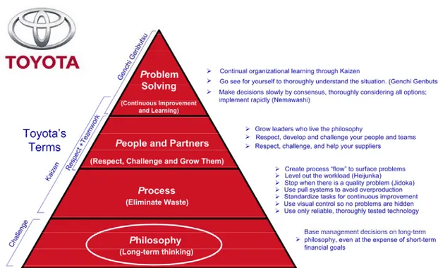
The LEAN thinking way doesn’t only focus on improving a process, but it is actually a wider approach to the production system, focussing on everything that is involved in it. In order to make a company more ‘LEAN’ the 4-P model (Philosophy, Process, People and Partners, Problem Solving) has to be adopted. The concept at the basis of this model is clearly explained in the pyramid sketch shown in Fig. 1.1, which summarize the way of thinking and the hierarchy in the LEAN approach.

(22)

The Toyota Way is a list of rules to be followed and accepted in order to act with a LEAN approach. Those rules are explained in the so-called 14 Principles, organized in four broad categories (one for each ‘P’ of the 4-P model):

1.3.1 Section I: Long-Term Philosophy

• Principle 1. Base your management decisions on a long-term philosophy, even at the expense of short-term financial goals.

1.3.2 Section II: The Right Process Will Produce the Right Results

• Principle 2. Create a continuous process flow to bring problems to the surface.

• Principle 3. Use “pull” systems to avoid overproduction.

• Principle 4. Level out the workload (heijunka). (Work like the tortoise, not the hare.)

• Principle 5. Build a culture of stopping to fix problems, to get quality right the first time.

• Principle 6. Standardized tasks and processes are the foundation for continuous improvement and employee empowerment.

• Principle 7. Use visual control so no problems are hidden.

• Principle 8. Use only reliable, thoroughly tested technology that serves your people and processes.

(23)

1.3.3 Section III: Add Value to the Organization by Developing Your People

• Principle 9. Grow leaders who thoroughly understand the work, live the philosophy, and teach it to others.

• Principle 10. Develop exceptional people and teams who follow your company’s philosophy.

• Principle 11. Respect your extended network of partners and suppliers by challenging them and helping them improve.

1.3.4 Section IV: Continuously Solving Root Problems Drives Organizational Learning

• Principle 12. Go and see for yourself to thoroughly understand the situation (genchi genbutsu).

• Principle 13. Make decisions slowly by consensus, thoroughly considering all options; implement decisions rapidly (nemawashi).

• Principle 14. Become a learning organization through relentless reflection (hansei) and continuous improvement (kaizen).

This thesis only focusses on Section II, as its purpose is to improve the processes related to some Aircraft Level analyses.

(24)

1.4 Specify value

The first step in the LEAN approach is to specify value. In order to do that it’s important to define who is the customer and what are his needs. In general the customer is the individual or group that receives what the process delivers. The customer can be either an internal or an external one, in each case it is important to agree together how the product has to be to meet the customer's needs at a specific price at a specific time.

It is important to understand what in the process is value adding, what is non-value adding and what is waste.

Value adding is defined as any process that changes the nature, shape or

characteristics of the product, in line with customer requirements.

Non-value adding is any work that is unavoidable with current technology or

methods that doesn’t increase the product value but adds cost or time.

Waste is the use of any material or resource beyond what the customer requires

and is willing to pay for. It can be removed immediately.

The amount of time given by value added, non-value added and waste is the lead

time.

Value added

Non-value added + waste

Fig. 1.2: Lead Time

1.5 Value stream map

Once the value had been identified there is the need to create a map of the value stream, through the current process. A Value Stream Map (VSM) is a visual aid

(25)

capturing all the steps both value-creating and non value-creating, required to bring a product from concept to launch and from order to delivery. Each action is represented by a block that has an input (coming from the previous block) and an output (going to the following one), and contains information about the CT (Cycle Time, time in possession), the TT (Touch Time, time actively at work) and the number of people involved in every action.

In the VSM the beginning of the flow is represented by the supplier and the end by the customer. At the bottom of the map there is a section underlining which fraction of the time adds value, which doesn’t and which one is waste.

The value stream map gives a snapshot of the whole process, underlining clearly where it’s needed to act in order to develop and improve the process. An example is given in Fig. 1.3 (in which the CT is identified with C/O and the TT with C/T).

Fig. 1.3: Value stream map

1.6 Improving the process

Only after specifying value and mapping the stream can lean thinkers implement improvements by making the remaining, value-creating steps flow.

(26)

From the analysis of a value stream map it can be seen easily that most of the time the sources of waste are due to incorrect management of the product during its development. Often it happens that a product remains still waiting for other people to control it, or for the next process in the chain to need it, and this causes interruptions in the flow.

Improving the process means both to act on these sources of waste and try to reduce or eliminate them and to reduce the time linked with value adding and non- value adding activities. The former is the improvement with the biggest impact in the very early stages of the development of the process; the latter becomes more consistent after some iterations of the process improvement practice.

At the end of the lean thinking revising process the product’s chain has improved and the lead time has been reduced.

A new value stream map can be produced. The aim is then to keep applying new methods and techniques to continuously improve the whole system.

The power of the lean thinking is in the possibility to apply the described approach at every level of a business, such as the manufacturing chain, the design phase of a single component or of a complex system, the development of a product or the building of a model.

In this work the lean approach is used for building the models and for running the analyses with them, using as baseline the models used in the ‘as-is’ process and trying to propose alternative methods to improve it.

In the following chapters some examples of LEAN thinking are applied to the processes, and an evaluation of the improvements brought with the new approach is made.

Further improvements can be obtained either by applying the LEAN philosophy to all the steps of the projects or by refining the already modified approach.

(27)

2 A350XWB Groundline analysis

Fig. 2.1: A350XWB Groundline analysis

2.1 Introduction

A groundline analysis is a static analysis that aims to sort out a set of data such as the forces acting on the landing gears, the closures of the shock absorbers, the position of some particular loaded points and the pitch angle of the aircraft for different combinations of input parameters. This analysis is very important in order to give information about the stability of the aircraft on the ground and to build the diagrams on how to load the aircraft in terms of fuel, passengers and cargo.

2.2 Value stream map

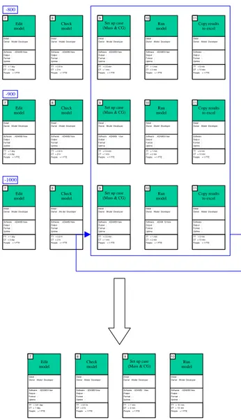
The ‘as-is’ process for A350XWB Groundlines analyses is reported in the Value Stream Map in Fig. 2.2.

(28)

For the analysis it is assumed that a validated model is available, and that there is the required budget.

The inputs for the analysis are given from the Landing Gear Structural Installation team (EDLSI) that manages ATA32 Installation, the Landing Gears design data (such as tyres and LG dimensions, LG mass, Shock absorbers data) provided by the design office, the A/C design data (masses, CG envelopes) and there may be external requirements (steering cam analysis, tyres burst cases or jacking groundlines, see Chapter 3).

The first step in the global process consists in finding and extracting the appropriate model from the model database for each aircraft version, then a Statement of Work (SoW) has to be provided from the design office with all the requested cases to be analysed.

The risks related to these phases are that the SoW may be late or incomplete, therefore needing to be double-checked and causing delays. There is also the risk of budget of resources not being available (in terms of manpower).

After these steps the data needed to feed the model have to be collected and put in the required format (excel spreadsheets), and the models have to be modified with what has changed from the previous status, and this operation has to be done for all the variants of A350XWB (-800, -900, -1000).

Afterwards the analyses have to be run, and therefore every model has to be set up with the required value of mass and CG position (which means modifying the position of the marker representing the CG, according to the required percent of MAC stated in each case). The results have to be manually collected, by extracting the values from the tool’s postprocessor and filling in an excel spreadsheet.

A final check of the measures has to be done, and when the NLG shock absorber shows a low closure a further loop is carried out changing manually the CG position until the minimum load is obtained in order to allow the correct steering cam behaviour. The following steps concern formatting the data for the required output format, and updating of the report with the new values. Finally the report is checked against the geometry, reviewed and approved and delivered to the customer.

(29)

Software : Output : Format : Uptime : Detail : Owner :Model Developer

TT = 1 min CT = 2 min People = 1 FTE 12 Change CG Legend:

TT = Touch Time (Time actively in work) CT = Cycle Time (Time in possession)

Lead time = 15646 min = 260.8 hr = 7.5 weeks = 1.863 months

Potential lead time reduction Up to 77.12%

A350XWB Groundlines analyses

Current State Value Stream Map

Assumptions : Validated ADAMS model available (Binary file)

Budget is available Generic Risks : EDLSI Customer Inputs EDLSI ATA32/Installation LG Design Data A/C Level design data

Requirements Software: Output: Format: Uptime: Detail: Owner:Model Developer

TT = 0.5 hr CT = 2 hr People = 1 FTE 1 Find model Software: Output: Format: Uptime: Detail: Owner:Model Developer

TT = 1 min CT = 2 hr People = 1 FTE 2 Extract model Software: Output: Format: Uptime: Detail: Owner:Model Developer

TT = 1 day CT = 2 weeks People = 1 FTE 5 Collect data Software: Output: Format: Uptime: Detail: Owner:Model Developer

TT = 1 day CT = 1.5 day People = 1 FTE 6 Format data Software: ADAMS/View Output: Format: Uptime: Detail: Owner:Model Developer

TT = 1 day CT = 3 day People = 1 FTE 7 Edit model Software : ADAMS/View Output : Format : Uptime : Detail: Owner :Model Developer

TT = 0.5 hr CT = 2 hr People = 1 FTE 8 Check model Software :ADAMS/View Output : Format : Uptime : Detail : Owner :Model Developer

TT = 0.5 min CT = 1 min People = 1 FTE 9 Set up case (Mass & CG) Software : ADAMS/View Output : Format : Uptime: Detail: Owner :Model Developer

TT = 1 min CT = 2 min People = 1 FTE 10 Run model Software : Output : Format : Uptime : Detail : Owner :Model Developer

TT = 5 min CT = 10 min People = 1 FTE 11 Copy results to excel Software : Output : Format : Uptime : Detail : Owner :Model Developer

TT = 3 hr CT = 1 day People = 1 FTE 12 Check measures Software : Output : Format : Uptime : Detail : Owner :Model Developer

TT = 2 hr CT = 1 day People = 1 FTE 13 Format data for report Software : Output : Format : Uptime : Detail: Owner :Model Developer

TT = 0.5 day CT = 1 day People = 1 FTE 14 Update report Software: Output: Format: Uptime: Detail: Owner:Model Developer

TT = 1 hr CT = 3 hr People = 1 FTE 15 _Cross check against geometry Software: Output: Format: Uptime: Detail: Owner:Model Developer

TT = 1 hr CT = 7 day People = 1 FTE 16 Review & Signatories Software : Output : Format : Uptime : Detail : Owner :Model Developer

TT = 0.5 day CT = 1 day People = 1 FTE 21 _Email report to customer Software: Output: Format: Uptime: Detail: Owner:Model Developer

TT = 1 min CT = 2 hr People = 1 FTE 3 Receive SoW Software: Output: Format: Uptime: Detail: Owner:Model Developer

TT = 2 hr CT = 2 day People = 1 FTE 4 Check SoW Budget not available Manual entry error of input SoW late/bad Lack of process WASTE 12066 NVA VA 2882 698 30 min 90 min 38 min 38 min 210 min 210 min 75 min 75 min 375 min 375 min 1 min 119 min 1 min 119 min 120 min 720 min 420 min 3780 min 420 min 210 min 1260 min 2520 min 90 min 270 min 180 min 240 min 30 min 90 min 60 min 120 min 60 min 2880 min 210 min 210 min Software: ADAMS/View Output: Format: Uptime: Detail: Owner:Model Developer

TT = 5 min CT = 10 min People = 1 FTE 11 Copy results to excel Software: ADAMS/View Output: Format: Uptime: Detail: Owner:Model Developer

TT = 5 min CT = 10 min People = 1 FTE 11 Copy results to excel -800 -900 -1000 x number of cases (20-25) x number of iterations (4)

Potential lead time reduction (only eliminating waste)

(30)

After defining what adds value, what’s non value adding and waste a first estimation of the potential reduction in time spent for the process can be made. The total time required by value adding actions is 698 minutes, the non-value adding bits require 2882 minutes and the waste is of 12066 minutes. If ideally the waste was eliminated the saving in lead time would be of 77.12%.

It has to be noticed that the estimation of time required to perform the analysis is rough and refers to an average analysis type. In fact, depending on the progress of the development of the aircraft the data changing from the previous status can be more consistent, and therefore the modifications to be implemented in the model will take more time in the very early stages of the design. On the other hand, the more the aircraft is defined in details, the less changes are made from one status to the following one.

The improvements proposed only refer to the central part of the global process, as the collecting data phase and the delivery are not analysed. These steps in the ‘as-is’ process take 488 minutes of value adding time, 1350 minutes of non value adding time and 3278 minutes of waste, without considering the loop for the steering cam analysis.

The aim of the new method is to automate as much as possible the analysis, trying to eliminate all the manual parts and speeding up all the steps.

In order to compare more appropriately the advantages of the new approach the time spent in the building of the models should be taken into account, as the parameterisation in the models requires more time with respect to the current process. Nevertheless, as it is assumed to have validated models ready for the analysis, only time spent for setting up and running all the cases is measured. The new method aims to build a single parameterised model that can be representative of all the versions of the aircraft, and to set up and run a set of simulations with all the cases of interest. The results have to be carried out and stored automatically in the desired format.

The tool ADAMS/Insight is used for this purpose, further details about the usage of the tool will be provided in the following paragraphs of this chapter.

(31)

2.3 Request of work

The work to be performed is a parametric analysis of the Groundlines for the 3 different versions of the A350XWB aircraft. The first parameterisation has to relate the values of all the geometric and mechanical parameters to another parameter that defines which version (–800, -900 or –1000) of the A350XWB is being analysed, the second parameterisation aims to cover all the design points issued by each one of the CG envelopes, and therefore consists in the possibility of varying the values of mass and CG position.

The request of work, the sources of the data and the main assumptions to be made are provided by a Statement of Work: the document explains all the different cases to be analyzed, it contains the official documents with the geometry data, the spring curves for the gears and the CG envelopes, and it describes how the analysis has to be performed.

In order to validate the model the results have to be compared with the ones given by the existing non-parameterised model for the status 11.

2.4 Input Data

The main input data for the model are the geometric architecture of the gears, the diagrams with the CG positions, the spring curves of the shock absorbers and the tyres information (in terms of stiffness and stiffness coefficient).

2.4.1 Geometric Architecture of the gears

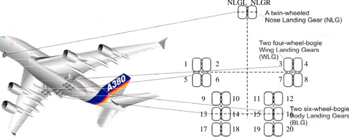
The architecture of the gears is the same for the versions –800 and –900 of the aircraft. The Nose Landing Gear doesn’t have any rake angle and two Main Landing Gears have 4 wheels each and a rake angle. The A350XWB-1000 version differs from the others for having 6 wheels for each MLG.

All the versions have a bogie angle that had been considered in the model even if it doesn’t affect the analysis.

(32)

Version Gear Status Document A350XWB-800/-900/-1000 NLG Baseline data -

A350XWB-800 MLG Baseline data -

Table 2.1: Geometry data sources

Moreover, the data for the coordinate systems of the aircraft (the nose frame, the main frame and the fixed frame) are obtained from the Data Basis for Design (DBD) of the A350XWB Status 10.

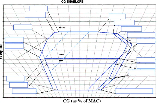
2.4.2 CG Envelopes

The CG diagram shows all the possible combination of CG position and total mass allowed for the aircraft. This helps to understand the behaviour of the aircraft during all the different loading conditions.

The CG envelopes are issued both in A350XWB_CG_Envelopes_Status_11.pdf and in the DBD.

2.4.3 Spring curves

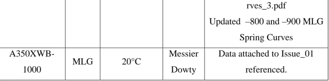
The spring curves describe the behaviour of the shock absorbers for each different load case at each different temperature. The non-linear behaviour of the curve suggests to make a best fit of the data retrieved from experiments. Data are taken form the following documents:

Version Gear Temperature Supplier Document

A350XWB-800/-900/-1000 NLG 20°C Liebherr

Data attached to A350-LLI Vendor Data Pack A350XWB-800/-900 MLG 20°C Messier Dowty Data attached to A350XWB_MLG_Spring_Cu

(33)

rves_3.pdf Updated –800 and –900 MLG Spring Curves A350XWB-1000 MLG 20°C Messier Dowty

Data attached to Issue_01 referenced.

Table 2.2: Spring curves data sources

2.4.4 Tyres Mechanical Data

The curves that explain the behaviour of the tyres are extracted from the Landing Gear System Data for A350 XWB Wheels, Brakes & Tyres – Report (V32RP0627988 iss 3 A350XWB WT&B Dat).

For each tyre data are taken from the following attachments:

Version Gear Tyre Attachment

A350XWB-800 NLG 1050x395 R16 28PR Bridgestone

11.4Bar (Unloaded) 11.9Bar (Loaded) - A350XWB-900 NLG 1050x395 R16 28PR Bridgestone

11.7Bar (Unloaded) 12.2Bar (Loaded) -

A350XWB-1000 NLG

1050x395 R16 28PR Bridgestone

11.8Bar (Unloaded) 12.3Bar (Loaded) - A350XWB-800 MLG 1400x530 R23 40PR Bridgestone

14.6Bar (Unloaded) 15.2Bar (Loaded) - A350XWB-900 MLG 1050x395 R16 42PR Bridgestone

14.6Bar (Unloaded) 15.2Bar (Loaded) -

A350XWB-1000

50x20 R22 PR34 Bridgestone 13.7Bar (Unloaded) 14.2Bar (Loaded)

MLG -

Table 2.3: Data sources for the tyres

(34)

2.5.1 Strategy

The main parameterisation has to relate all the parameters to the one indicating which version of the aircraft is being analyzed. The ideal approach would be to use IF-THEN-ELSE logical switch operators to instruct the model to assume a certain set of parameters when a certain situation occurs (IF the aircraft is A350XWB-800 THEN…., ELSEIF…).

The tool MSC ADAMS/View 2005 r2 gives the chance to choose a set of parameters and assign them the desired values, but since the parameters are created by design-time functions, there’s not the possibility to use the logic IF operator, which belongs to run-time functions, and so the only way to build a parameterised model which could automatically switch from a set of parameters to the others, just by varying the Aircraft Version parameter is to use a polynomial function like the following, also known as Lagrange Polynomial Function:

∏

∑

≠ ≠ − − ⋅ ⋅ = i j j i i j j i i x x x x x x P P ) ( ) ( where:

• P is the desired value for the parameter

• Pi is the value of the parameter when x equals a certain xi

in this analysis the expression is then:

20000 ) 800 )( 900 ( 1000 10000 ) 800 )( 1000 ( 900 20000 ) 900 )( 1000 ( 800 3 2 1 − + ⋅ x− x− x x x x x x x − − ⋅ − − ⋅x P x P x P

where P1, P2 and P3 are the values of a certain parameter in the –800, -900 and – 1000 version, and x is the value of the parameter Aircraft_Version_DV. With this

(35)

expression the design variable assumes the value P1 when the A350XWB-800 is selected, P2 when it’s the –900 and P3 by choosing the –1000 version.

P1, P2 and P3 are parameters themselves, and that allows to change each single parameter for each aircraft version without affecting any other variable.

An example of this parameterisation is provided in Fig. 2.3.

Fig. 2.3: Example of parameterised function

he second parameterisation allows the user to change manually the position of the

ge rapidly the value of a certain

2.5.2 Geometry

he first step in the building of the model is the creation of the geometry.

is called

ong the AC axes

e is the one for the coordinates of the MLG, and it is positioned

ed in the

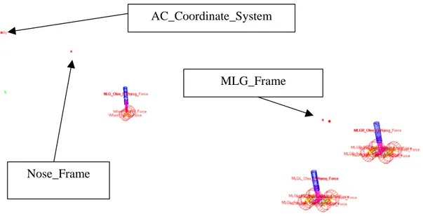
ordinate frames can be seen in Fig. 2.4. T

centre of gravity and the total mass of the aircraft. The purpose of this parameterisation is both to chan

parameter for a single analysis and to allow the user to run a batch run with all the required simulations for every parameter set of each aircraft version.

T

First of all the reference frames have to be set. The main one

AC_Coordinate_System, and is set in the origin of the model, with the global orientation. All the other reference frames are related to this one.

The Nose_Frame reference frame’s position is parameterised al

with the parameters Nose_Attach_X_DV, Nose_Attach_Y_DV and Nose_Attach_Z_DV. This frame is the one to which the coordinates of the NLG are referred and therefore is very relevant when switching from an aircraft version to another one.

The MLG_Fram

along the AC X axis at a parameterised distance (Main_Frame_X_DV). The values of the parameters to position the coordinate frames are issu DBD.

(36)

AC_Coordinate_System

Nose_Frame

MLG_Frame

Fig. 2.4: A350XWB-800 Coordinate frames

The NLG had been bu ment. This marker is

arametrically positioned with respect to the Nose_Frame (the function

MLG_Frame), but the ilt from the marker NLG_Fuse_Attach

p

LOC_RELATIVE_TO had been used), as issued in the DBD. A cylinder (NLG_Main_Fitting) is built form this marker, and another one (Strut) is built coaxial to the Main Fitting, connected to it with a translational joint in order to allow only the movement along the axis direction. The Strut is constrained with a fixed joint to the axle, a cylinder at the top of which are fixed (with fixed joints) the wheels. Again the length of the cylinder is fixed once its top and bottom markers are defined with the positions issued by the document in Table 2.1. The gear does not have a rake angle and since there are only 2 wheels there is not any bogie beam. The wheels are modelled as cylinders, but their roles in the model are fictitious, as the tyres loads are applied directly to the axle.

The MLG has a similar architecture for the leg (the reference marker is MLG_Fuse_Attachment, and the reference frame is the

constraint with the bogie beam is a revolute joint, in order to allow the bogie beam to have a DOF with respect to the Strut. The bogie beam is a cylinder built between two specific markers, and the axles of the wheels are linked to it with fixed joints. As for the NLG, the axles are cylinders at the top of which the wheels are fixed with fixed joints, and the tyre loads are applied. Since for the –800 and –900 versions the wheels for each one of the main gears are 4 the bogie beam has 2

(37)

axles, in the –1000 the wheels are 6, and the axles are therefore 3. In order to take into account this difference the wheel’s radius for the central wheels of the MLG is zero when the Aircraft_Version_DV parameter is different from 1000.

The gears are the only components modelled in details; the rest of the aircraft is just the total mass (less the un-sprung mass of the gears), concentrated in the CG (with parameterised position). The part Aircraft is then constrained to both the gears with a fixed joint at the top of each Main Fitting.

The model for each gear is represented in Fig. 2.5.

Fig. 2.5: Geometry of the gear for A350XWB-1000

.5.3 CG and total mass data

percent of the Mean Aerodynamic Chord AC). To calculate the distance from the Nose Frame (Xcg in the Nose_Frame

2

The position of the CG is given as a (M

Coordinate System) it is used the following:

(

)

⎟ ⎠ ⎞ ⎜ ⎝ ⎛ _⋅ + −

= X MAC MAC MAC

Xcg MAC 100 % 25 . 0 25

(38)

where X25MAC and MAC are provided by the Status 10 DBD and are the position of the 25% of the MAC and its length.

ince the components cannot have zero mass all the elements of the Landing Gears

s all the masses are negligible if compared to

Aircraft) is connected to the main fittings of the gears with fixed

2.5.4 Sprin

order to model the behaviour of the shock absorbers of both the MLG and the NLG in static conditions, the data collected by the static spring curves at the S

are given a fictitious mass of 0.5 kg. This affects neither the total mass of the aircraft nor the position of the CG, a

the total mass.

The mass is modelled as a sphere positioned on the CG of the aircraft. In its properties the total mass (less the gears un-sprung mass) is given to the sphere, and this part (called

joints on the Fuse_Attachment markers.

An example of a typical CG envelope is shown in Fig. 2.6.

CG (as % of MAC)

Weights

Fig. 2.6: Example of a typical CG Envelope

g Curves

(39)

temperature of 20°C are taken into account, but the data relative to other mperatures, other pressures or other vendors can be easily loaded on the model

a best fit of the points provided by the te

and switched with the opportune parameter.

The spring curves give the oleo force versus the relative displacement of the cylinders of each leg of the gears. The modelled behaviour is then the one of a non-linear spring with variable stiffness and a fictitious damping.

The data are collected from the curves with

shock absorber’s provider, attached in the related documents. These points are loaded in ADAMS/View as splines, and fitting the data then automatically produces the related forces.

The typical spring curves are shown in Fig. 2.7 and Fig. 2.8.

Fig. 2.7: NLG static spring curves

7 0 .0 6 0.0 50 . 0 40 .0 30.0 20 . 0 10 .0 0 .0 -1 0 .0 - 20.0 -30 . 0 -4 0 .0 - 54.0 D yn am ic b raki ng JA R 25.4 9 3 d M R W =2 45.9 t, xC G = 2 2% M AC , F S/ A= 7 160 53 N R ef . V 32 R P0 62 768 4,I ssu e 1 , 30 . N ov . 200 6 2 .00 * m a x. s tat ic lo a d lo a d Η = 1.0 s ta tic lo ad at -30 °C fo r Η =1.0 R e f. V 32M E 072 273 2, Issu e 1, 1 3.A ug .2 0 0 7 m ax. st atic lo ad = 240 157 N R ef. V32M E07 2 2 732, Is sue 1, 13. Au g. 20 07

S AT m ax m in . sta ti c lo ad = 7 44 95 N R ef. V32M E07 227 32, I ss u e 1, 1 3. Au g .200 7 st at ic lo a d M TO W , a ft C G = 15 276 4 N R ef . V 3 2M E 0 722 732 , Is su e 1, 13 .Au g .20 0 7 s tati c lo a d a t -54 °C f or ≅ = 1 .0 R e f. V32 M E0 72 2732 , Issu e 1 , 13 .Au g .2 007

Shock absorber travel

Sho

ck absorber L

(40)

A350-800 XWB MLG Status 10 Static Spring Curve 0 500 1000 1500 2000 2500 3000 3500 4000 0 0.1 0.2 0.3 0.4 0.5 0.6 0.7 0.8

Shock Absorber Closure (m )

Sh o ck Ab so rb er L o a d (kN)

Nominal 20 deg C -30 deg C -54 deg C MTOW static load MTOW 1.15g load MTOW 1.7g load AFTOW 1.15g load

AFTOW assumed to be 220T. Current spring curve meets a fatigue w eight of 213T for a 1.15g load at -54

(41)

Since the interest of the analysis is focused on the static behaviour of the gears, the transient due to the ‘drop’ of the aircraft is not of interest, therefore the damping force of the shock absorber is modelled as:

2

cV

F =

where c is a fictitious damping coefficient and V is the relative velocity between the two cylinders of each leg of the gears. The force goes to zero as soon as the aircraft reach the equilibrium.

To model the shock absorbers in ADAMS two forces are applied between each Main Fitting and each Strut. It doesn’t matter between which markers the forces are applied, it’s just necessary that one belongs to one part and one to the other, and that they are positioned on the common axis of the cylinders. The value of the stiffness force is defined with state variable MLGL_Oleo_Stiffness_Force_SV. The structure of this state variable is defined with the expression

-AKISPL(MIN(MAX(VARVAL(MLGR_Oleo_Stroke_SV),-Max_Stroke_DV), MAX_Stroke_DV),0,MLG_Oleo_Stiffness_800_Spline,0).

This function takes the value by interpolating (with a linear interpolation) the figures of the spline MLG_Oleo_Stiffness_800_Spline that contains the spring curves data. If the displacement between the components excesses the maximum displacement allowed the force is the one related to the maximum displacement. Fig. 2.9 gives an example of the shock absorber loads.

(42)

2.5.5 Tyres

Plotting the empirical data for the tyres (force vs deflection) a very good compliance of their behaviour with the function y=cxn in the range of interest for this analysis can be observed, where:

• y is the force • c is the stiffness

• x is the deflection of the tyre • n is the stiffness coefficient

Therefore the results can be plotted in a bi-logarithmic scale so that the tyres show a linear behaviour, compliant to the function Y = AX +B. It is then sufficient to make a best fit of the curve, to measure its slope (A) and the intersect with the X axis (B) and then evaluate the stiffness and the stiffness coefficient as:

B

c=10

A

n=

this can be seen in Fig. 2.10

Logy

Logx

(43)

The tyre is then modelled again as a non-linear spring with a known stiffness and stiffness coefficient.

As a damping coefficient a fictitious one is chosen. In fact this damping affects only the transient in whom the aircraft moves towards the equilibrium, after which the situation is static and the damping forces are zero.

The forces are then modelled as impact forces, normal to the ground, applied to the axles in the centre of the wheels, and can be seen in Fig. 2.11.

Fig. 2.11: Tyre forces

2.6 Results request

The requested results for the analysis are:

• The X position of the CG in the AC Axis

• The position of the loaded and unloaded point E (in the middle of the central axle) for both the MLG and NLG from the Main_Frame and the Nose_Frame respectively

• The closures of the shock absorbers in each gear • The loads of the shock absorbers in each gear • The Static Loaded Radius (SLR) of the tyres

(44)

• The Pitch Angle of the aircraft

2.6.1 CG position in AC Coordinate Frame

This measure gives the steady position of the CG of the aircraft along the AC Coordinate Frame. This position is affected by the pitch of the aircraft, which causes the CG to slightly move along the horizontal axis. This measure is taken by tracing the displacement along the X axis of the marker CG.

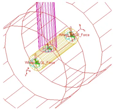
2.6.2 Loaded point positions

The loaded point is a conventional point taken in the centre of mass of the axle for the NLG and of the bogie beam for the MLG. Since the model is symmetric and symmetrically loaded about its longitudinal plane only the X and the Z components of the displacement of that point is relevant. The loaded points are shown in Fig. 2.12 and Fig. 2.13

MLG Loaded point

(45)

NLG Loaded Point

Fig. 2.13: Loaded point of the NLG

The measure is simply taken by tracing the displacement of the marker positioned in the loaded point.

For the NLG the measure of the loaded point’s position is made with respect to the Nose_Frame, for the MLG the reference frame is the MLG_Frame.

2.6.3 Shock absorber’s closure

The measure of the closure of the shock absorbers is made by measuring the relative displacement between any two points belonging to the Strut and to the Main Fitting of each leg, along the direction of the leg’s axis

2.6.4 Tyre’s Static Loaded Radius

The tyre’s SLR is the distance between the centre of mass of the axle and the ground after the tyre’s deformation. This measure indicates the radius of an equivalent fictitious rigid tyre once the equilibrium is reached

(46)

2.6.5 Unloaded point positions

This measure is a design parameter rather than a result, as it is the position of the loaded point before the beginning of the simulation. This measure is useful to compare the changing of the position of that point during the simulation.

As for the loaded point, for the NLG the measure of the unloaded point’s position is taken with respect to the Nose_Frame, for the MLG the reference frame is the MLG_Frame.

2.6.6 Shock absorber’s load

This is a measure of the elastic load transmitted between the two components of the leg at the equilibrium. For the nature of the force and for how the model had been built this is the closure of the shock absorber times the stiffness in that condition.

2.6.7 Pitch angle

The pitch angle is the angle between the direction of the longitudinal axis of the aircraft and the ground. At the beginning this angle is zero, then it changes to its steady value.

2.7 Simulation

2.7.1 Single run

The analysis consists in dropping the aircraft from a certain height (this to avoid numerical issues related to the initial conditions which would occur by placing the aircraft already on the runway with the tyres in contact with the ground), and waiting for the equilibrium to be reached after a transient during which the variables are not of interest. To set up a simulation the total mass, the CG position

(47)

and the aircraft version have to be chosen, then the simulation parameters such as the step size and the duration of the simulation have to be decided and finally the simulation is started.

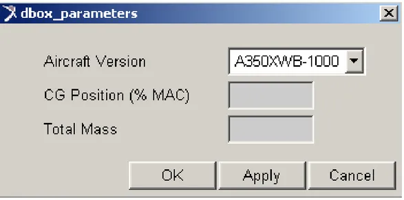
In order to have a rapid parameters variation a GUI is produced with the values for the above mentioned variables:

Fig. 2.14: GUI for rapid parameters variation

o customize the simulation parameters a simulation script is written. There is the

ond with 1000 steps (the step

t is in 2.6.

2.7.2 Batch run

batch run simulation with all the parameter sets required in the Statement of

n the simulation are: T

necessity of a smaller step size in the first part of the simulation (the transient) due to the rapid variation of the variables. The following part of the simulation can be performed more rapidly, and with a bigger step size.

The first part is performed with a simulation of 1 sec

size is 1/1000 seconds) and the second part is of 100 seconds still with a 1000 steps (the step size is then 1/10 seconds).

The description of the results reques

A

Work has to be run with the ADAMS/Insight Tool. The main parameters that change in every case run i

(48)

• Aircraft_Version_DV (800, 900 or A350XWB-• t_Total_Mass_DV (The mass of the aircraft)

CG in percentage of

he selection of these parameters is shown in Fig. 2.15: 1000)

Aircraf

• CG_Position_Perc_MAC_DV (The position of the MAC)

T

Fig. 2.15: Parameters selection in ADAMS/Insi t

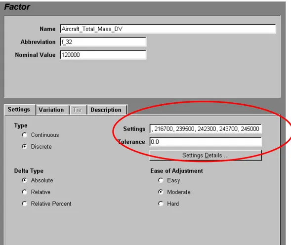
the options of the Factors the allowable values of the parameters have to be

n chosen and their variation ranges have been

osing a DOE Response Surface and Latin Hypercube in the window shown

en be edited as an excel spreadsheet, and therefore the cases gh

In

indicated as shown in Fig. 2.16. Once the parameters have bee

indicated the setting up of the analysis goes on with the definition of the analysis type.

By cho

in Fig. 2.17 an editable workspace is automatically created, with a number of trials set up in random points of the dominium that is equal to the number indicated in the options.

The workspace can th

(49)

Since the result of the batch run is a table only single values can be stored in it, therefore only initial, final or average value can be recorded in this analysis. If the history of a certain measure has to be analysed either a single run can be performed or the result file .res can be opened in another ADAMS/View file and then analysed in the postprocessor.

This procedure could be really useful, but a .res file will be saved for each single simulation case, and this may cause an excessive size of the folder that contains the data.

(50)

Fig. 2.17: Analysis options

(51)

Eventually the analysis has to be run and the results have to be analysed and converted in the appropriate format.

2.8 Validation

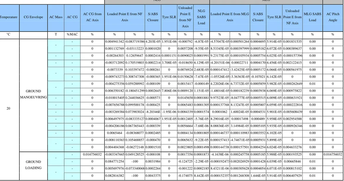
The results of the model are compared against the results of the same simulations, made for the same analysis cases but with the validated non-parameterised model. Those results have already been peer-reviewed and actually populate the DBD of the A350XWB. The results are compared and an error table is produced. In the table there are the percentage error between the results of the validated non-parameterised model and the new one. Only the Pitch angle shows an absolute error, as the values are so little that the percentage error would be relatively big. The percent error between the results of the parameterised model and the non parameterised one are reported in Table 2.4

(52)

NLG MLG

Temperature CG Envelope AC Mass AC CG AC CG from AC Axis

Loaded Point E from NF Axis S/ABS Closure Tyre SLR Unloaded Point E from NF Axis NLG SABS Load

Loaded Point E from MLG Axis S/ABS Closure Tyre SLR Unloaded Point E from NF Axis MLG SABS Load AC Pitch Angle °C T %MAC % % % % % % % % % % % % % %

- 0 0.004941342 -0.083719386 4.203E-05 1.951E-06 -0.000792 -6.87E-05 -4.57047E-05 0.000501264 0.0004695 5.914E-05 0.001831535 0.00 0 -

- 0 0.001132769 -0.03113223 0.0001020 0 0.0057208 -9.55E-05 8.53345E-05 0.000397999 0.0005182 6.072E-05 0.000389637 0.00 0 - - 0 -0.00264303 0.12659647 0.0002416 0.0001151 0.0090025 0.0001991 9.23175E-05 0.000105934 0.0005754 6.025E-05 -0.000157396 0.00 0 - - 0 -0.003712092 0.170519803 0.0002214 3.708E-05 -0.018650 6.129E-05 -4.20151E-06 0.00022711 0.0004170 6.456E-05 0.002122415 0.00 0

- 0 -0.0073339 0.103397472 -0.000261 0 0.0076924 2.683E-05 0.000147412 -3.42425E-05 0.0005172 6.066E-05 0.000561975 0.00 0 -

- 0 -0.009743273 0.308747308 -0.000365 1.951E-06 0.0150628 -7.67E-05 -1.05526E-05 -3.36363E-05 -0.107021 6.142E-05 0 0.00 0 - 0 -0.004275356 0.059288992 -0.000109 0 0.0015417 -0.000149 4.22026E-06 6.73732E-05 0.0005859 5.982E-05 -0.000262649 0.01 0 -

- 0 0.006350182 -0.180451299 0.0002645 7.806E-06 0.0009120 1.151E-05 -1.48016E-05 0.000182239 0.0003938 6.069E-05 0.000975822 0.00 0 - - 0 -0.010015405 0.244036625 -0.000573 0 0.0145658 0.0001881 9.97523E-05 -8.04777E-05 0.0005515 6.009E-05 -0.000631921 0.00 0 - - 0 -0.007656788 0.099500178 -0.000425 0 0.0065483 0.0001305 0.000137768 8.13247E-05 0.0005807 6.059E-05 -0.000222816 0.00 0 - - 0 -0.003269384 0.073903024 -8.20346E -1.95E-06 0.0084339 0.0001574 0.0001062 1.60024E-05 0.0004531 5.901E-05 -0.005608439 0.00 0 - - 0 0.006497975 -0.083335127 0.0004067 1.951E-05 0.0012405 -5.76E-05 8.29016E-05 0.00017498 0.000489 5.958E-05 0.002954588 0.00 0 - - 0 -0.004206186 0.067365443 -0.000339 0 0.0056664 -7.68E-06 8.08836E-05 3.14984E-05 0.0005105 5.935E-05 -0.000926346 0.00 0

- - 0 0.0065464 -0.08368077 0.0002485 0 0.0004134 0.0001805 0.000146737 0.000110983 0.0003552 6.102E-05 0 0.00 0

- 0 -0.008110363 0.105468857 -0.000470 0 0.0065632 -9.22E-05 0.000157413 -4.74671E-05 0.0005931 5.899E-05 0 0.00 0

GROUND MANOEUVRING - - 0 0.004404368 -0.06272148 0.0001510 0 0.0023805 0.0001498 0.000144738 0.000157501 0.0004254 6.024E-05 0.004633276 0.00 0 - 0.016756032 -0.003347665 0.049128525 -0.000108 0 0.0017356 0.0001873 -4.1638E-06 0.000245758 0.0005185 5.988E-05 0.000193525 0.00 0.016756032 - - 0 0.084771254 -100 0.0031984 0 -0.124725 -2.29E-05 -0.000192473 0.002026929 0.0001428 6.039E-05 0.00665846 0.01 0 - 0 0.005697976 -0.073340068 0.0002264 0 -0.001222 0.0002185 8.43211E-06 0.000305628 0.0004054 6.071E-05 0.000815102 0.00 0 20 GROUND LOADING -

- 0 0.082816382 -100 0.0043375 0 -0.174075 8.442E-05 -0.000152357 0.001268308 1.646E-05 5.914E-05 0.006407929 0.01 0

Table 2.4: A350XWB-800 Percentage error table1