1
Introduction
Recently wireless communications have become one of the main research topic, due to the great variety of services and applications that they provide. Flexibility and scalability are the main reasons of their success. Moreover, the user’s demand is constantly growing up, looking forward for new features and needs. Next – generation wireless communications targets to improve link throughput and network capacity in order to provide the users with a fast and flexible connection, suitable for many different services and demands.
The development of Multiple Input Multiple Output (MIMO) systems has been an important headway in wireless communications because they hardly increase the data throughput without increasing the bandwidth demand or the transmission power. The high spectral efficiencies attained by a MIMO system are due to the fact that signals from different transmitters appear strongly uncorrelated at each of the receive antennas. This is possible in a rich scattering environment, with the spatial multiplexing (SM) transmission technique. Moreover, MIMO systems can be employed also to improve the bit error rate (BER) performance, make a more reliable transmission and combat the channel fading. Space – time coding is the main technique to achieve these improvements. Because of these features, MIMO is an important part of modern wireless communication standards like IEEE 802.11n, WiMAX, 3GPP Long Term Evolution (LTE) and International Mobile Telecommunication Advanced (IMT – Advanced).
This work starts from the results of the DAVINCI project. DAVINCI (Design And Versatile Implementation of Non-binary wireless Communications based on Innovative LDPC Codes) project, which is a Seventh Framework Program (FP7) ICT Collaborative project funded by
2
the European Commission. DAVINCI’s goal was to set up foundation of non-binary digital wireless transmission to achieve the high spectral efficiency requirements of next – generation wireless communications. In particular it focused on an IMT – Advanced systems implementation.
The main advantage of non-binary coding is the superior performance of non-binary processing at the receiver, due to the fact that the decoder takes into account the correlation between bits. It has been shown that, at similar system complexity, non-binary information processing can outperform the Shannon limit of its binary counterpart. Moreover the decoding process can be faster than the binary one for adequately selected parameters. The main issue is to combine space – time codes and channel codes jointly in order to achieve a great complexity reduction in the receiver processing. The soft demapper computes the a-posteriori probability (APP) log-likelihood values (L-values) that are a sufficient statistic of the received signal and form the input of the decoder. The computation of the L-values can be strongly improved using a direct mapping, that is a one to one correspondence between a transmit vector and a code symbol.
Results proving these advantages are shown in the deliverables of the project and set a starting point for future research in this field.
Following the system model of the DAVINCI project, in this work we focus our investigation on space – time coding schemes. Our intent is to present a capacity comparison of different space – time coding schemes both for coded modulation (CM) and binary interleaved coded modulation (BICM) systems and focusing on MIMO systems 2x1 and 2x2. The performances of a communication system depend on the capacity of the equivalent channel, which include the effects of the space – time block codes, the channel and the soft demapper. So, in our results, we present the capacity computed for the whole equivalent channel that is a memoryless discrete-input continuous-output channel.
3
The main objective of this thesis is to design the best space – time code for a given system in order maximizes the Discrete-input Continuous-output Memoryless Channel (DCMC) capacity of the equivalent channel.
To do this we investigate the Spatial Multiplexing, Alamouti and Linear Dispersion Codes schemes with different constellations, i.e. PSK, QAM and Sphere Packing.
In particular, we analyze the framework of the Linear Dispersion Codes and present an algorithm to find a code that maximizes the DCMC capacity, both for CM and BICM systems.
To compute the capacity in an efficient way we use Land and Kliewer algorithms that lead to low time-consuming simulations to get the mutual information.
Since the performance of a LDPC code depends mostly on the mutual information per coded bit, i.e. on the capacity of the equivalent channel between the encoder and the decoder, we can calculate an estimation of the WER of the channel for which we already get the capacity. It is useful to avoid simulations that could take too much time.
Our work was carried out in the Radio Communication laboratory of the Centre Tecnologic de Telecomunicacions de Catalunya (CTTC). To simulate the channel and compute the capacity and the WER of the investigated transmission systems we used the MATLAB development environment.
This thesis is structured as follow. In chapter 1 we introduce the multiple-input multiple-output systems. Then, in chapter 2, we describe the system model and its component. In chapter 3, we present the capacity definition and the methods we used for an efficient computation of the capacity. In chapter 4, we focus on Linear Dispersion Codes (LDC). First we analyze their structure and then we describe how to design a good LDC using a random search algorithm for the maximization of the DCMC capacity. In
4
chapter 5, results are presented and discussed. In the conclusions, we summarize the entire work, focusing on the most interesting results found.
5
Chapter 1
Multiple-Input Multiple-Output systems
Digital communications exploiting multiple-input multiple-output (MIMO) wireless channels has attracted considerable attention as one of the most significant technical discovery in modern communications. After its development, it was clear that this technology could be part of a large-scale of standards of commercial wireless products and networks such as broadband wireless access systems, wireless local area network (WLAN), third generation (3G) networks and so on. In the context of wireless transmissions, it is common knowledge that depending on the surrounding environment, a transmitted radio signal usually propagates through several different paths before it reaches the receiver, which is often referred to as multipath propagation. The radio signal received by the receiver antenna consists of the superposition of the various paths. If there is no line-of-sight (LOS) between the transmitter and the receiver, channel coefficients corresponding to different paths are often assumed to be independent and identically distributed (i.i.d.). In this case the central limit theorem applies and the resulting path gain can be modeled as a complex Gaussian variable (which has an uniformly distributed phase and a Rayleigh distributed magnitude). Due to this statistical behavior, the channel gain can sometimes become very small so that a reliable transmission is not always possible. To deal with this problem, communication engineers have thought of many possibilities to increase the so-called diversity. With higher diversity, the probability of a small channel gain is lower. Some common diversity techniques are time diversity and frequency diversity, where the same information is
6
transmitted at different time instants or in different frequency bands, as well as spatial diversity, where we make the assumption that fading is at least partly independent between different points in space. The concept of spatial diversity leads directly to an expansion of the SISO system. This enhancement is denoted as single-input multiple-output (SIMO) system. In such a system, we equip the receiver with multiple antennas. It leads to a considerable performance gain, but also co-channel interference can be better combated. At the receiver, signals are combined and the resulting advantage in performance is referred to as the diversity gain obtained from independent fading of the signal paths corresponding to the different antennas. System improvements are not only limited to the receiver side. If the transmitter side is also equipped with multiple antennas, we can either be in the multiple-input single-output (MISO) or multiple-input multiple-output (MIMO) case. Diversity gain is achieved with the use of space – time block coding. Besides the advantages of spatial diversity in MIMO systems, they can also offer a remarkably gain in terms of information rate or capacity. This improvement is linked with multiplexing gain, and it is attained with the use of the spatial multiplexing technique. The underlying mathematical nature of MIMO systems, where data is transmitted over a matrix rather than a vector channel, creates new opportunities beyond the just described diversity effects. Wireless systems that employ multiple antennas are able to achieve higher transmission rates because of the improved bit/symbol capacity compared to the single-input single-output (SISO) systems. The employment of multiple antennas offers a linear increase in spectral efficiency, compared to a logarithmic increase in more traditional systems utilizing receive diversity or no diversity. The main reason of the higher spectral efficiency achieved by a MIMO system is that, in a rich scattering environment, the signals from each individual transmitter appear highly uncorrelated at each of the receive antennas. In this scenario, signals are sent through uncorrelated channels between the transmitter and the receiver, so that signals from different transmit antenna
7
are spatially uncorrelated. The receiver is able to separate signals originated from different transmit antennas.
One of the most important transmission technique used in wireless communications employing MIMO systems is the above-mentioned space – time block coding. It consists in transmitting multiple copies of data streams across a number of antennas and use the various received versions of the data to improve the reliability of data-transfer. Space – time coding combines all the copies of the received signal in an optimum way to extract as much information as possible from each of them. Transmitting multiple redundant copies of data is useful to combat fading and thermal noise. Data stream that has to be transmitted is encoded in blocks, which are distributed over spaced antennas and across time. While to improve the performance it is necessary to have multiple transmit antennas, it is not necessary to have multiple receive antennas. Space – time block codes are capable to provide the diversity gain, which improve the achievable system performance in terms of signal reliability and robustness of the transmission.
Another very popular transmission technique is the spatial multiplexing (SM). It is designed to improve the attainable spectral efficiency of the systems. It consists in transmitting different signals streams independently over each of the transmit antennas in order to get a multiplexing gain and so achieve better performances.
In this chapter we present the multiple antennas model and the characterization of multiplexing gain and diversity gain. Finally we introduce the space – time block codes.
1.1
Multiple antennas model
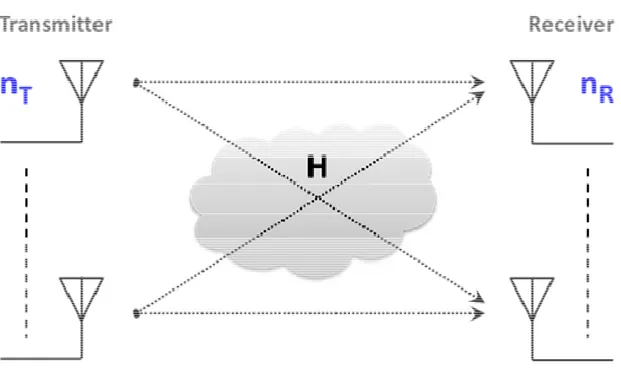
To define the model of a multiple-input multiple-output communication system, let us consider a system with n transmit and T n receive antennas as depicted in Figure 1. Now R
8
we assume to have a narrow-band flat fading channel, constant for at least T channel uses. We can write:
SNR
T
n
Y = HS + W (1.1)
where Y∈ℂnT×T is the received signal, S∈ℂnT ×T is the transmitted signal, and R
n ×T
∈
W ℂ is the addictive white Gaussian noise (AWGN) at the receiver. The noise is modeled as a white circular Gaussian random variable with zero-mean and No 2 variance per real and imaginary component. The Gaussian distribution for the disturbance term can often be motivated by the central limit theorem.
The channel matrix H∈ℂnR×nT has independent entries, modeled as Gaussian random variables with zero-mean and unit-variance. The generic element of
H
,h
i j, , is the channel gain between thei
th receive andj
th transmit antenna.We are assuming a frequency-flat fading channel. This assumption can be made when the delay spread of the channel is negligible with the inverse bandwidth. Anyway, if we have a frequency-selective channel it is possible to use an OFDM (Orthogonal Frequency Division Multiplexing) system to turn the MIMO channel into a set of parallel frequency-flat MIMO channels, in which our model can be still applied.
Under the assumption of a frequency-flat Rayleigh fading channel the elements of
H
can be modeled as zero-mean circularly symmetric complex Gaussian random variables with variance of both real and imaginary part equal to
1/ 2
. Consequently, the amplitudes, i j
h
are Rayleigh-distributed random variables. Note that we are considering a rich scattering environment, where there are no line-of-sight components between9
transmitter and receiver. In addition, in (1.1) we do not consider the dependency on time because we assume a time-invariant channel in T signaling intervals.
We have the following constraints on our elements of the MIMO transmission model: - average magnitude of the channel path gains
{
tr H}
R T n n
Ε HH = ; - average transmit power
{
tr H}
T n T
Ε SS = .
The factor SNR n in (1.1) ensure that SNR in the average signal to noise ratio at a T receive antenna, independent of the number of transmit antennas.
10
1.2
Multiplexing Gain and Diversity Gain
The two types of gain that can be achieved using MIMO systems: the diversity gain and the multiplexing gain. Following the notation of [1], we analyze the two different approaches of employing MIMO systems.
Multiple antennas systems have been employed with the purpose of increasing diversity in order to combat channel fading, using for example an appropriate space – time block code. Each pair of transmit and receive antennas provides a signal path between the transmitter and the receiver. Signals with the same information are sent through different paths and multiple replicas of the data symbol, weighted with independent fading coefficients, can be obtained at the receiver. In this way we can achieve a more reliable data transfer. The diversity gain is related to the number of independent fading coefficient that can be averaged over to detect the symbol. In a general system arranged with nT transmit and nR receive antennas, the full diversity gain provided by the channel is: n nT R, which is the total number of fading coefficient of our channel. To be more precise, we say that a MIMO system achieves a diversity gain of d if:
(
)
SNR log SNR lim log SNR e d →∞ Ρ = − (1.2)where Ρe is the average error probability. So (1.2) represent the slope of the average error probability in log-scale at high SNR regimes. This means that, for an uncoded system, given two STBCs with different diversity gain, we can find the effect of this difference in the slope of their BER curves.
Multiple antenna systems can also be employed to improve the data rate. In this case we have to adopt the spatial multiplexing scheme that consists in the transmission of
11
independent information symbols in parallel through the spatial channels. Let us consider the ergodic capacity (in bit/s/Hz) of the ergodic block fading channel, in which each block is as in (1.1) and the channel matrix is i.i.d. across blocks:
(
SNR)
log det
nRSNR
H TC
n
Ε
+
HI
HH
≜
(1.3)Considering high SNR values, (1.3) can be written as:
{
}
max{ , }{
2}
( )
2 1
SNR
min , log log 1
T R T R n n i T R T i n n n n o n + =
∑
− + Εχ
+ (1.4)where χ2i is chi-square distributed with 2i degrees of freedom. So, while for single
antenna channels the capacity increase with log SNR , for multiple antenna it increase with min
{
n nT, R}
log SNR. It can be considered as a set of min{
n nT, R}
parallel spatial channels. We call min{
n nT, R}
the total number of degrees of freedom to communicate. This scenario represent a situation in which the fading coefficients of each path between a transmit and a receive antenna are independent, so that the channel matrix is well conditioned with high probability and multiple parallel spatial channel are created. The spatial multiplexing technique is the most appropriate to benefit of this scenario. Now to define the multiplexing gain, let us R(
SNR)
be the transmission rate, expressed in bit/symbol. We say that a MIMO system achieves a multiplexing gain of m if:(
)
SNR SNR lim log SNR R m →∞ = (1.5)12
we know that the maximum achievable rate Rmax
(
SNR)
of a system is its capacity, sowe can interpret the maximum multiplexing gain as the slope of the system capacity when the SNR goes to infinity. The maximum achievable multiplexing gain is m=min
(
n nT, R)
.1.3
Space – time block codes
Spatial multiplexing scheme is only able to achieve a diversity gain of n instead of the R full n n diversity, and a transmit diversity of one. This motivates to search space – time T R block coding schemes that are able to achieve the full transmit diversity. The basis of space – time coding is to find a way to spread the data symbols over space and time and, at the receiver side, to have a simple processing of data. The coding scheme can be seen as a way of mapping set of Q symbols
{
s s1, ,...,2 sQ}
onto a matrix S∈ℂnT×T. We define the spatial rate of the space – time block code as:(
)
min , S T R Q R n n T = [symbols/channel use] (1.6)In the case of RS=1, the code is named full rate.
Linear space – time block codes are a subclass of STBC. The transmission matrix T
n ×T
∈
S ℂ is formed according to:
{ }
{ }
(
)
1 Q i i i i i s j s = =∑
ℜ + Ι S A B (1.7)13
where
{
A Bi, i}
, i=1...Q form a set of matrices with domain ℂnT×T. They spread the real and imaginary part of the complex data symbols onto the transmitted matrix S .An important subclass of linear STBC are the Orthogonal space – time codes (OSTBC). The underlying idea started with the work of Alamouti, and was extended later to the define the general class of OSTBC. A space – time block code is orthogonal if satisfy:
2 1 T Q H i n i s = =
∑
SS I (1.8)It means that the space – time signal matrix S is an orthogonal unitary matrix, able to separate the data streams of the multi antenna symbols into independent single antenna symbols. This class of STBC achieve optimum performances also with receiver that employ linear equalizer, like Zero Forcing (ZF) or Minimum Mean Square Error (MMSE).
Now we focus on the Alamouti scheme, that is the first and one of the most used OSTBC. The transmission matrix of the Alamouti OSTBC for the case of two transmit antennas is: 0 1 1 0 s s s s ∗ ∗ − = S (1.9)
It considers the transmission of two complex symbols in two time slots, so it is a full rate code. Referring to (1.7), the modulation matrices for the Alamouti scheme can be identified as: 1 2 1 2 1 0 0 1 1 0 0 1 , , , 0 1 1 0 0 1 1 0 − = − = = = A A B B (1.10)
14
The construction of an OSTBC for a number of transmit antennas greater than two is difficult, moreover we know that there are no space – time block codes full rate for a number of transmit antennas different from two. Alamouti code, using the optimal decoding scheme, provides the same diversity order of the maximal ratio receiver combining (MRRC) with one transmit and two receive antennas. This is due to the perfect orthogonality of symbols after the receive processing. Moreover Alamouti code is the only STBC able to achieve the full diversity gain without losing in data rate, in the case of
1 R
n = . This scheme does not require any feedback from the receiver to the transmitter and its computation complexity is similar to MMRC.
The decoding processing is simple and offers great results. Referring to a 2 1× system and according to (1.1), we can write the received symbols as follow:
* 0 0 0 1 1 0 * * 1 0 1 1 0 1 y h s h s w y h s h s w = + + = − + + (1.11)
The combining scheme is structured as follow:
* * 0 0 0 1 1 * * 1 1 0 0 1 s h y h y s h y h y = + = − ɵ ɵ (1.12)
This leads to the decision variables:
(
)
(
)
2 2 * * 0 0 1 0 0 0 1 1 2 2 * * 1 0 1 1 0 0 1 0 s h h s h w h w s h h s h w h w = + + + = + − + ɵ ɵ (1.13)15
We can observe that the signal power increases by
(
)
2
2 2
0 1
h + h and the noise power increases by h02+ h12, moreover, as we expected from an orthogonal code, there are no
16
Chapter 2
Modeling Encoded MIMO Communications
In this work we consider a coded transmission system over a MIMO channel. The transmitter scheme consists in a channel encoder followed by an interleaver and a mapper. Then, symbols are sent through a Rayleigh fading channel. At the receiver there is a soft demapper, which calculates the L-values and then a de-interleaver. Finally there is the channel decoder, producing the estimation of the transmitted information symbols.
The investigated system scheme is shown in Figure 2.
a
b Figure 2. Block diagram of the transmission system.
17
Figure 2a considers a Coded Modulation (CM) system, with the symbol-wise interleaver. Figure 2b considers a Binary Interleaved Coded Modulation system, in which there is a bit-wise interleaver. In this case, before the decoder, there is a block that convert the binary L-values into q -ary L-vector. In this section we will explain better the components of both the transmission systems and the differences between them.
The channel we consider is a Multiple-Input Multiple-Output channel characterized by
T
n transmit and n receive antennas. R
Using a vector notation we describe the received signal at the channel output as:
=
+
y
Hx w
(2.1)Where y∈ℂnR×1 is a complex vector and its elements are the received symbols at each antenna.
Then H∈ℂnR×nT is the complex channel matrix as described in the first chapter.
The complex vector x∈ℂnT×1 represents the transmitted symbols.
The complex vector
∈
nR×1w
ℂ
represents the noise at the receive antennas. Its elements can be modeled as white circular Gaussian random variables, i.e.(
0,
0)
R nN
Ν
w
∼ ℂ
I
18
2.1
FEC coding
Forward error-correction coding (FEC), also called channel coding, is a type of digital signal processing that consists in the introduction of redundant bits in order to improve data reliability.
The decoder at the receiver can detect and possibly correct errors that occur due to the noisy transmission channel. The main advantage of this scheme is that the receiver does not need a re-transmission of data, leading to a save of bandwidth.
The two main types of channel codes are the block codes and the convolutional codes. In this work we will focus on the Low-Density Parity-Check (LDPC) linear block codes.
A block code transforms a sequence of K information symbols in a sequence of N coded symbols, called a code word. This kind of block code will be denoted with ( ,K N . ) We define the rate of the code r K 1
N
= < .
The LDPC code is so called because it is defined by a very sparse parity-check matrix. The generator matrix of the code can be written as:
( )
[ K K×N K− ]
=
G I P (2.2)
where PK×(N K− ) is a binary matrix. The parity check matrix is given by:
T
( )
[ N K− ×K K] =
D P I (2.3)
The decoder, once received the vector y , makes the parity check, defined by the equation:
19
T =
Dy 0 (2.4)
The decoding processing consists in an iterative algorithm called Belief Propagation (BP). First to describe the decoding algorithm, let us introduce the Tanner Graph, an alternative way to represent the relationship between the bits of a codeword and the parity check equation. It is a bipartite graph composed by two classes of nodes: the bit nodes, related to the coded bit, and the check nodes, referred to the parity check equation. The design rule is quite simple, the check node j is linked to the bit node i if the element di j, of the parity check matrix is equal to one. The decoding algorithm is
based on passing probability or likelihood messages between bit nodes and check nodes. In fact, the messages exchanged are vectors of probabilities calculated using logarithm of a-posteriori probability ratio (LAPPR) criterion. Due to the particular structure of the decoder, it is better to avoid cycles in the Tanner Graph because they lead to worst performance of the decoding processing, in terms of computational time. LDPC codes can approximate the Shannon limit, if decoded with the iterative message-passing sum-product algorithm and they are capable of parallel implementation for a higher decoding speed.
The NB-LDPC codes, [2], are a generalization of the binary ones. The parity check equations are written using symbols over Galois Fields of order q , denoted F , and for q the particular binary case we have q=2. Starting from (2.4), we can write the i -th parity check equation: , , : 0 0 i j i j j j d d y ≠ =
∑
(2.5)20
Now we extend this notation to the non-binary case, that is considering elements taken from the Galois field F . It is possible to represent the symbol q y using j log q -tuples 2
( )
defined over F , as presented in [3], [4]. So let us consider the (2.5) in the vector domain: 2, T T , :i j 0 i j j j d D ≠ =
∑
y 0 (2.6)where Di j, is the log2
( )
q ×log2( )
q matrix over the binary field associated to the F q element di j, , and y is the vector representation of the symbol element j y . Considering j the i -th parity check equation, we define Di=[
Di j, 0,...Di j, m,...Di j, nc −1]
as the equivalentbinary parity check matrix, where jm:m=0...nc−1 are the indexes of the nonzero elements of the i -th row and nc is the number of check nodes (it does not depend on i if we consider a regular code). Then we define Yi=
[
yj0,...yjnc −1]
the binary representationof the binary symbols involved in the i -th parity check equation. Finally we have found the binary representation of the i -th parity check equation, which can be written as:
T T
i i =
D Y 0 (2.7)
There are two main advantages in the use of non-binary coding. First, it have been observed [5], [6], that regular codes with two bit nodes are very sparse and this leads to a Tanner Graph with very large girths, compared to usual binary codes graphs. This means that the decoding process has better performances. Moreover, the binary image method to design the code lead to an improvement of the performances both in the waterfall and the error floor region, compared to the random method for the choice of the Tanner Graph structure and the assignment of the non-zero values, used to design binary codes.
21
The improvement of the performance using non-binary coding leads to an increased decoding complexity. The same decoder structure is used for both binary and non-binary coding, that is the Belief Propagation decoder. The main difference is that for the non-binary BP decoder the messages between bit and check nodes are defined by q−1 L-values or q probability weights. A good complexity reduction can be obtained by using a sub optimum decoder, the Extended Min-Sum (EMS) decoder, which use only a limited number of L-values in the message exchange. It have been shown [6] that it offers the best tradeoff between complexity and performance.
In this work we use an NB-LDPC code designed in Galois field of order q=64, which correspond to the largest modulation order considered for wireless communications.
The encoder takes a message K q
∈
u F consisting in K q -ary Galois Field symbols and
encodes into a codeword N q
∈
c F of N code symbols. The code we used has the following parameters: N =480, r=1 2.
2.2
Interleaver
It is known that many communication channels are not memoryless; this implies that errors typically occur in burst and not independently.
Interleaving is a process of scrambling the order of data sequence. It produces an enhancement of the error correcting capability of the decoder because it creates a more uniform distribution of errors. The inverse of this process is denoted by de-interleaving. It consists in the scrambling of the received sequence in order to restore the original one.
In this work we consider an ideal interleaver, modeled by a random switch. Obviously the receiver knows the scrambling rule for de-interleaving the received sequence.
22
In the case of the binary processing the interleaver is a bit interleaver, so we are considering a Bit-Interleaved Coded Modulation (BICM), [7]. This is the case depicted in Figure 2b.
Otherwise we are considering a symbol-wise interleaver for a Coded Modulation (CM), as shown in Figure 2a.
2.3
Modulation and MIMO Scheme
In this work we compare different MIMO coding schemes with different modulations. We have used standard QAM, PSK and Sphere Packing (in two and four dimensions) modulations. The QAM and PSK constellations are assumed to have a gray mapping.
Spatial multiplexing, Alamouti and Linear Dispersion Codes schemes have been investigated and compared.
Simulations have been carried out with the same transmitted energy for a fair comparison.
2.4
Mapping and Soft Demapping
We consider a mapping of m1 coded GF symbols
(
)
T1
,
2,....,
m1b b
b
=
b
taken fromF
q,to a vector of m2 QAM/PSK/Sphere Packing modulation symbols
(
)
T1
,
2,....,
m2x x
x
=
x
, sothat x=µ
( )
b . The vector x differs from the one of the model of (2.1) only for his length. This is to describe a general case, in our system we will consider the particular case of23
2 T
m =n . We will explain later the reasons of this choice. Named M the cardinality of the constellation, we are considering a mapping that satisfy 1 2
M
m m
q = .
To describe a system in which the modulation symbols are allocated in more than a single transmit vector, e.g. for
m
2>>>>
nT, it’s useful to consider this matrix notation as in (1.1): Y SNRHS W T n = + = + = += + , where S is a nT××××T matrix containing the
m
2 modulatedsymbols.
The soft demapper computes the A Posteriori Probability (APP) L-vector
(
, 0, , 1,..., , 1)
i= Li Li Li q−
L which corresponds to the coded GF symbol b . Following the i model of [8], we can define the components of the L-vector for the i -th GF symbol by:
( )
{ }( )
{ } : : 0 ,ln
i i b k b i k p pL
= ==
∑
∑
S S Y S Y S (2.8)Computing the L-vector is a very time consuming operation, but we can achieve a great complexity reduction if the vector
x
forms the transmit vector, so that T ====1 and nT ====m2,in addition to m1====1. In this case S= =x µ
( )
b and one coded GF symbol b∈∈∈∈F is q mapped in exactly one transmit vector and the set{
S: b=k}
reduces to one element. So (2.8) can be simplified as follow:(
)
{
}
(
)
2 2 0 0 0 1 ( ) (0) 1 2 ( ) ( ) ( ) k H H H L k N k k k Nα
= − − − − = ℜ − + y Hµ y Hµ y Hµ µ H µ (2.9)24
where
α
0 is a constant that does not depend on k . This notation is useful because weare using a decoder that is invariant to additive constant, so that
α
0 can be omitted in thecomputation of the L-values. Since one coded GF symbol is mapped into all components of the transmit vector, this is called vertical mapping.
For binary processing, the L-vector is replaced by a scalar L-value, which is defined by:
1 ln 0 i i i P b L P b = = = y y (2.10)
Given a memoryless scalar channel yj =h xj j+wj with xj =
µ
j( )
b , j=1,...,m2, andassuming that code symbols are equiprobable, it is possible to compute (2.10) in this way, [8]:
( )
{
}
{
( )
}
0 1
jac log jac log
i i i L p p ∈Β ∈Β = − b b y b y b (2.11) where
{
1}
2 : k m i bi k Β = ∈b F = and( )
2( )
2 1 1 m j j j j p y b = − No∑
= y −hµ
b . Moreover, the Jacobian function is so defined: jaclogx A ln exp( )x A x
∈ =
∑
∈ .In chapter 5 we evaluate the differences between binary and q -ary information processing at the receiver. For this purpose we are assuming to use the same q -ary LDPC codes for both cases; this means that we are decoding with the same q -ary decoder. It is possible since we are considering F , with q power of two, in our case q q=64. In the binary case we have to reconstruct the L-vectors from the binary L-values. It is carried out
25
by viewing a coded GF symbol b∈F as a vector of q log2
( )
q bits and computing their binary L-values. Then the q -ary L-vector is given by:( ) ( ) 2 2 ( bin ) log , log , , , 1 1 ln 0 q i j j q i k j i j i j j j P b k L k L P b = = = = = =
∑
∏
yy (2.12)where for k∈F q we denoted the corresponding bit vector by
(
)
2( ) 2 log 1, 2,..., log ( ) 2 q qk k k ∈F . For single antenna systems with BPSK or QPSK modulation, binary demapping leads to the same performances of the q -ary. For multiple antennas is sub-optimum for all modulations.
As shown in [2], [6], for multiple antennas systems, non-binary processing jointly with non-binary coding is significantly superior to binary processing. For example, in many cases the BER curves of non-binary systems beat the BICM Shannon limit. It means that there is no binary code of arbitrary length able to achieve the performance of those NB-LDPC codes.
26
Chapter 3
Capacity Computation
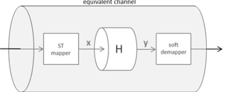
In this section we will investigate the capacity of the MIMO system described above. Two methods for a fast capacity computation will be presented, taking into account the equivalent channel, which consists of the space – time mapper, the MIMO channel and the soft demapper, as depicted in Figure 2.
Figure 3. Equivalent channel
3.1
MIMO channel capacity
The channel capacity is the maximum of the mutual information I x y
( )
, over all possible input distributions.27 ( )
( )
max , pdf C I x x y ≜ (3.1)From information theory we know that this maximum is achieved with a Gaussian distribution of the channel input.
Thus, the capacity of the MIMO channel can be written as:
( )
SNRmax log det R
x T H n x tr n T C n = = + C H I HC H [Bit/s/Hz] (3.2)
Where
C
x is the covariance matrix of the transmitted vectorx
defined by{ }
H xΕ
C
≜
xx
.The Signal to Noise Ratio (SNR) is given by:
0
SNR
n E
T SN
≜
(3.3)Where E represents the transmit power per antenna, i.e. S ES = Ε
{ }
xi2 .For a fading channel, the channel matrix
H
is random, and so also the associated capacity defined in (3.2) is a random variable. For that reason we define the ergodic channel capacity as the average of (3.2) over the distribution ofH
:SNR
max log det
RT x H E n x tr n T
C
n
= Ε
+
H CI
HC H
≜
(3.4)28
If the channel matrix
H
is known at the transmitter, is possible to choose the transmit correlation matrix C that maximize the channel capacity, for example using the x technique of “water-filling”. For this method the perfect channel state information (CSI) has to be sent back to the transmitter, and it implicates a complex system with a feedback channel.In our work we assume the perfect channel state information only at the receiver side. In case of perfect CSI at the receiver side, it has been demonstrated that the optimal signal covariance matrix is the identity matrix, i.e.
C
x=
I
nR. This means that the antennas should transmit uncorrelated streams with the same average power.What we obtain is not the Shannon capacity, anyway is the best we can do with no CSI at the transmitter.
Finally the ergodic channel capacity of our system is given by:
SNR
max log det
RT x H G n tr n T
C
n
= Ε
+
H CI
HH
≜
(3.5)This expression has been obtained under the assumption of Gaussian distributed transmit signals. In our system, transmitted modulation symbols are taken from a finite alphabet of a QAM/PSK M-dimensional constellation ξ with equal probabilities. Hence we show the two expressions for the channel capacity in the cases of a Coded Modulation (CM) and a Bit Interleaved Coded Modulation (BICM), following the results and notations in [8].
29
(
)
0 2(
(
)
)
, , ,,
log
,
CMp
C
I
R
p
ξ ∈ = =
− Ε
x'∑
x y H x y Hy x' H
y x H
(3.6)where
I
(
x y H is the average mutual information, conditioned to the knowledge of ,)
the channel, that is perfect CSI at the receiver side. Then p( )
⋅ represents the probability density function. We denote by Rq≜log2( )
M the number of bits per symbol and0 T q
R =n R is the number of bits per channel use, assuming T =1.
To compute the BICM capacity we consider the parallel-channel model presented in [9], that simulate the behavior of an ideal binary interleaver. The model consists in R parallel 0
channel, each of them representing one of the R bit that have to be transmitted. Let S 0
be the random variable that determines the interleaving rule, that is in which channel the system have to transmit each bit. We consider S as a random variable i.i.d. uniformly distributed over
{
1,..., R0}
. Now let us consider the average mutual information of thebinary input b and the received vector y , conditioned to a particular realization of S :
(
)
(
(
)
)
, 2 , , , , , 1 log , i b b p I b S i p ξ ξ ∈ ∈ = Ε = −
∑
∑
x' y H x' y x' H y H y x' H (3.7)Averaging in respect to S we obtain:
(
)
0(
)
0 1 1 , , , , R i I b S I b S i R = =∑
= y H y H (3.8)30
Finally, considering R parallel channel, the BICM capacity, with perfect CSI at the 0
receiver, is given by:
(
)
0(
(
)
)
, 0 0 2 , , 1 , , , log , i b R BICM b i p C R I b S R p ξ ξ ∈ = ∈ = = − Ε ∑
∑
∑
x' y H x' y x' H y H y x' H (3.9)where ξi b, is the subset which contains the transmit vectors whose associated bit vector has the value b∈
{ }
0,1 in his i position.For a faster computation of the capacity we used the algorithm of Land [10] and its generalization for non-binary systems from the paper of Kliewer [11]. These algorithms compute the mutual information between the input of a channel encoder and a soft-output of a Log-APP decoder.
3.2
Efficient computation of channel capacity: BICM
To compute in a simple and efficient way the capacity in (3.9) we used the method proposed in [10] where the average symbol-wise mutual information between info bits and the output of a LogAPP decoder is investigated. It have been shown that this mutual information can be computed using only the absolute values of the L-values, which are the output of the LogAPP decoder. This is possible because an L-value contains the same information about a transmitted binary symbol as the whole received sequence does. This means that the L-value is a sufficient statistics of the received sequence. The only requirement to use this method is that the L-values of the info bits are available.
31
Considering the info bits bk∈ + −
{
1, 1 ,}
k=1,...,K, let us define the average symbol wisemutual information as:
( )
(
)
1 0 1 , K symbol k k k I I b L b K − = =∑
y (3.10)As proved in [10], we say that the mutual information between an info bit b and the k received word y and the mutual information between an info bit b and the respective L-k value L b y do not change when they are conditioned to the reliability
( )
k Λ =k L b( )
k y . That is:(
)
(
)
(
)
(
)
(
(
)
)
, , , , , , k k k k k k k k I b I b I b L b I b L b = Λ = Λ y y y y (3.11)Another useful results, proved in [10], is the following:
(
)
(
k, k, k)
I( )
kI b L b y λ = f λ (3.12)
where we consider λk a given realization of Λk and the function fI
( )
⋅ is so defined:( )
2 2 1 2 1 2 log log 1 1 1 1 I x x x x f x e+ e+ e− e− = + + + + + (3.13)Finally, we use can use the previous results and definitions to compute the average symbol wise mutual information:
32
( )
(
)
( )
(
)
( )
(
)
{
}
( )
{
}
( )
( )
{
}
1 0 1 0 1 0 1 0 1 0 1 , 1 , 1 , 1 1 K symbol k k k K k k k k K k k k k K k I k K k I k k I I I b L b K I b L b K I b L b K f K f K fλ
λ
λ
λ
− = − = − = − = − = = = Λ = Ε = Ε = Ε = Ε∑
∑
∑
∑
∑
y y y (3.14)The main advantage of this method is that the determination of histograms of the a-posteriori LLR is not required. The computation of the mutual information is carried out by simply averaging over a function of the absolute values of the a-posteriori LLRs.
We can compute the capacity of a BICM channel in this way:
( )
{
}
BICM I k
C = Ε f
λ
(3.15)As shown in [10], this method produces exact results, unbiased.
3.3
Efficient computation of channel capacity: CM
A generalization of the previous method for the non-binary case has been presented in [11]. This approach offers a more convenient way to compute the capacity in (3.6) thanks to information averaging.
33
As the previous one, also this method can be applied in a system, where the soft demapper provides the L-values L , used for the computation of the capacity. k
Starting form (3.6), we can write:
(
)
2 1 1 0 2 , 0 0 1 SNR log exp ln 2 q q R CM m i m i T n C R q n − − = = = − − Ε − − + ∑
v H∑
H x x v (3.16)where v∼ ℂN
(
0,InR)
, and we are assuming that there is a one-to-one mapping from the GF code symbol c and the transmit vector x , in the case of T =1, so that the number of possible transmit vector is q . Thanks to information averaging, as proposed in [12], we can compute (3.16) in this way:1 0 2 0 log q CM k k k C R p p − = = + Ε
∑
(3.17)where pk= Ρ =
(
x x yk) (
= Ρ =c ck y)
,k=0,1,...,q−1 is the a-posteriori probability of the GF code symbol c=ck. Finally, using the L-vectors computed by the soft demapper, the coded modulation capacity can be computed as follow:( )
( )
1(
)
2 0 1 log ln 2 k q L CM k k C q e Lβ
β
− = = + Ε − ∑
(3.18)Where β is given by:
1 0 k q L k e β − = =
∑
(3.19)34
Thanks to this method we can achieve a great complexity reduction in the computation of the capacity.
3.4
Capacity of Alamouti – equivalent channel
In this work we use the Alamouti scheme, [13], on MIMO 2 1× and 2 2× systems. With the Alamouti scheme two symbols are transmitted in two time slots and the receiver is able to conveniently combine the received signals. The computation of the capacity becomes faster. Thanks to the particular structure of the Alamouti space – time matrix, it is possible to compute the capacity considering the equivalent Soft Input Soft Output (SISO) channel. This is possible because the decoding processing provides two decision variables without cross terms between channels, as shown in (1.13).
For the 2 1× case, let us consider the Alamouti space – time matrix of (1.9). The receiver combines the received signals and obtains the vector y=
[
y y0, 1]
, whosecomponents are given by (1.11). After the combining scheme described in (1.12) it is clear that we can compute the capacity of this equivalent SISO channel, whose coefficient is
(
2 2)
1 2
eq
h = h + h .
A similar procedure can be carried out for a 2 2× system, where the combining at the receiver leads to an equivalent SISO channel coefficient heq=
(
h112+ h122+ h212+ h222)
.35
Thanks to the combining scheme at the receiver we have found an expression for the equivalent SISO channel, both for the 2 1× and 2 2× systems. Then to compute the CM and BICM we use the methods [10] and [11] presented above.
36
Chapter 4
Linear Dispersion Codes
In this chapter we describe the framework of Linear Dispersion Codes, in order to find a code that maximize the DCMC capacity. First, we present the channel model and the Linear Dispersion framework, then we describe the random search algorithm that aims to maximize the channel capacity.
The set of Linear Dispersion Codes (LDC), first proposed by Hassibi and Hochwald in [14], consists in a class of high – rate coding schemes that can handle any configuration of transmit and receive antennas and that subsume V-BLAST and many others space – time block codes as special cases. The main idea is to transmit substreams of data in linear combinations over space and time.
4.1
Channel model and Linear Dispersion framework
Before defining the capacity of a MIMO system employing LDC, we need to make a short overview of the channel model because the notation used for this model, described in [15], is slightly different from the one we proposed in the first chapter.
37
With Linear Dispersion Code we refer to a transmission of Q symbols in T time slots in a nT×nR MIMO channel. In this way different substreams of data are transmitted as linear combination over space and time.
An advantage of Linear Dispersion Codes is that they are suitable for any possible configurations of transmit and receive antenna, combined with any modulation schemes.
Let us define the transmitted space-time matrix S∈ℂnT×T, given the vector of M-PSK or M-QAM transmitted symbols K =
[
s s1, ,...,2 sQ]
T:1 Q q q q s = =
∑
S A (4.1) where nT T q∈ ×A ℂ are the specifics dispersion matrices. They spread the symbol s q over the n spatial and T temporal dimensions. T
The dispersion matrices have to satisfy the power constraints:
(
H)
q qtr A A =T Q. The received signal matrix Y∈ℂnR×T can be written as follow:
= +
Y HS W (4.2)
Where H∈ℂnT×nR is the channel matrix described in the second chapter. It is assumed to be constant during T symbols periods and change independently from one space – time matrix to the next.
The matrix W∈ℂnR×T represents the noise at the receive antennas for each time slots. The columns of W represent the realizations of an i.i.d. complex AWGN process with zero–mean and variance determined by the SNR .
38
Now we have to rewrite the (4.2) in an equivalent vectorial form:
= +
Y HχK W (4.3)
where ∈ n TR ×1
Y ℂ is the vector of the received symbols.
Then H∈ℂn T n TR ×T is given by: T
= ⊗
H I H, where ⊗ is the Kronecker product.
Matrix χ∈ℂn T QT × , called Dispersion Character Matrix, is defined as:
( )
1 ,( )
2 ,...,( )
Qvec vec vec
=
χ A A A , where the vec
( )
⋅ operation is the vertical stacking of the columns of an arbitrary matrix. This introduces two different power constraints on the matrix χ , depending on how we are arranging the system (if we are choosing Q<n TT or not).The vector W∈ℂn TR ×1 represents the AWGN at the receive antennas.
Equation (4.3) shows that the nT×nR MIMO system has been transformed into a R
Q n T× equivalent MIMO system. This notation is useful for the algorithm that we present in the next section, which aims to maximize the DCMC capacity.
4.2
Algorithm for maximizing the DCMC capacity
The method proposed in [16] to compute the capacity of a MIMO system with a LDC space-time mapper is based on a random search algorithm which maximizes the Discrete-input Continuous-output Memoryless Channel (DCMC) capacity.
The procedure takes into account the modulated signal constellation (QAM or M-PSK) so that the total number of possible combination for the transmitted symbol vector
39
K is F =MQ. This method is based on a coded modulation (CM) system. Later we will investigate the BICM case.
The DCMC capacity of the MIMO system, when we have the equivalent model of (4.3), is given by: 1 2 ( ),..., ( ) 1 1 1 ( , ) max ... ( ) ( ) log ( ) ( ) F F f LDC f f CM p K p K F f g g g p K C p K p K d T p K p K ∞ ∞ = −∞ −∞ = =
∑ ∫ ∫
∑
Y Y Y Y (4.4)Assuming equiprobable transmitted symbols vector Kf, f =1,...,F, the capacity (4.4) is simplified as:
( )
(
,)
2 2
1 1
1 1
log log exp
F F LDC f g f CM f g C F T F = = = − Ε
∑
∑
Ψ K (4.5) where Ψf g, is given by [17]:(
)
(
2 2)
, 1 f g f g No = − − + + Ψ Hχ K K W W (4.6)The random search algorithm we adopted consists in these steps:
40
- Under the assumption that Q<n TT the matrix χ can be generated taking the first Q columns of the unitary matrix obtained using the QR decomposition of χ and multiplied for a scale factor T Q. This satisfy the power constraint H
Q T Q
=
χ χ I ;
- If we arrange the system to satisfy Q=n TT the matrix χ is given by:
( )
1 QR T n =χ χ . This satisfy the power constraint: H 1 n TT
T n
=
χχ I ;
- In this way we are searching in the entire set of legitimate dispersion character matrices and we choose that one that maximizes (4.5).
From [15] we know that any dispersion character matrix χ that satisfy the power constraint is capable to approach the MIMO channel capacity, in the case of Q=n TT .
Otherwise, if we arrange a system with Q<n TT the ergodic capacity is approached within a margin proportional to Q T.
In order to use this method also for the BICM case, we get the expression of the capacity that has to be maximized from the general case of(3.9), considering the system model described by (4.3).
Since our system is able to compute the L-values at the soft demapper we can use the method proposed in [10] described above to get an efficient computation of the capacity for the BICM case.
41
Chapter 5
Numerical results
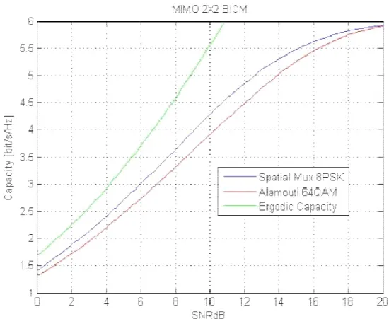
In this section we present the performances, in terms of capacity curves, of the space – time block codes we designed. Spatial Multiplexing, Alamouti and Linear Dispersion Codes schemes are compared for MIMO 2 1× and 2 2× systems, considering both the coded modulation and the binary interleaved coded modulation capacity.
5.1
Capacity of MIMO 2x1 systems
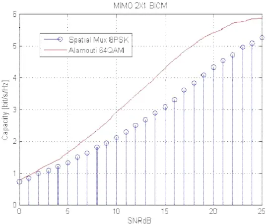
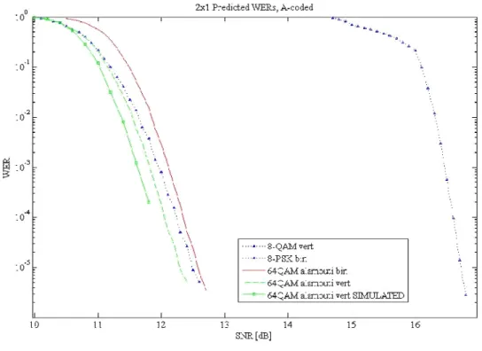
First, we investigated the MIMO 2 1× system. All simulations are carried out using constellation with gray mapping. We developed the algorithm to get the capacity of the channel with the Alamouti scheme, both for the BICM and CM case. For a fair comparison with a spatial multiplexing scheme, our simulations have been done with the same spectral efficiency. This means that we employed a 8-PSK (or 8-QAM) constellation mapping for the spatial multiplexing and a 64-QAM for Alamouti. That is due to the fact that with the Alamouti scheme we are transmitting two symbols in two time slots, on the other hand with spatial multiplexing four symbols are transmitted in two time slots. Choosing those constellations we ensure that the same number of bits is transmitted from each system.
In Figure 4 we present the capacity of a BICM system, showing that there is a huge gain in applying the Alamouti scheme, compared to the spatial multiplexing. There is a gap of
42
about 5 dB when the capacity is equal to 4 bit/s/Hz and this gap becomes bigger for higher values.
Figure 4. Capacity curves for 2 1× MIMO, Alamouti and spatial multiplexing.
Now we focus on the Alamouti scheme, to estimate what is known from a theoretical point of view about the superior performances of a CM system over a BICM.
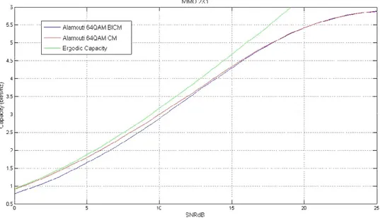
Figure 5 depicts the capacity of the Alamouti scheme computed for CM and BICM systems and the ergodic capacity of a 2 1× MIMO channel.
43
Figure 5. Capacity curves for 2 1× MIMO, Alamouti CM and BICM.
44
The CM capacity is strictly upper bounded by the capacity with Gaussian input. Moreover, as is shown in Figure 6, at a capacity of 1.5 bit/s/Hz there is a gap between CM and BICM of about 0.7 dB.
The better performances of CM expected from theory, are validated by our simulation. The capacity of coded modulation is equal or greater to the capacity of bit interleaved coded modulation, moreover this gap is suppose to increase for higher order modulations and in a system with a greater number of antennas. This is because BICM loose the information about the correlation of bits.
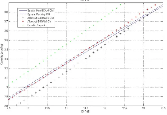
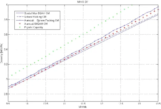
In Figure 7 we show that Alamouti BICM can achieve the capacity of a CM spatial multiplexing system for high SNR values. First we can conclude that Alamouti scheme always outperforms spatial multiplexing for the 2 1× case.
45
Figure 7. Capacity curves for 2 1× MIMO, Alamouti, spatial multiplexing and Sphere Packing.
We developed a two-dimension Sphere Packing modulation, [19], with 64 points, in order to make a comparison with the 64QAM modulation both with the Alamouti and spatial multiplexing schemes. In Figure 8 it is shown that Sphere Packing modulation has a very little gain when applied with spatial multiplexing. This gain increases is the Sphere Packing modulation is combined with the Alamouti scheme, in particular for higher SNR values.
46
Figure 8. Capacity curves for 2 1× MIMO, Alamouti with Sphere Packing.
In order to complete our investigation on 2 1× systems, we focus now on the design of Linear Dispersion Codes.
The target is to outperform Alamouti , which is the best scheme for the 2 1× systems. In the following, we identify a Linear Dispersion Code with LDC
(
n n TQT R)
, i.e. a transmission of Q modulation symbols of a given constellation during T time slots, over aT R
n ×n MIMO system.
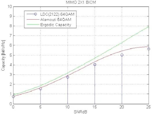
For the BICM, we design a code for the transmission of two 64QAM symbols during two time slots. In this case we can make a comparison with the Alamouti scheme using the same constellation. Figure 9 shows that LDC(2122) is not able to achieve the capacity of the Alamouti scheme.
47
Figure 9. Capacity curves for 2 1× MIMO, LDC(2122) 64QAM, BICM case.
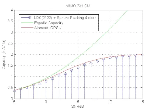
For the CM case, we tested a LDC(2122) with a QPSK and a Sphere Packing modulation. The Sphere Packing constellation is made of 4 symbols, with the same energy of the QPSK. Simulations show that there is no significant difference between the LDC employing the QPSK and the Sphere Packing constellation. Nevertheless, as presented in Figure 10 and Figure 11, Alamouti scheme is performing slightly better than LDC in both cases.
We can conclude that for a 2 1× system Alamouti is actually a good scheme and this
48
Figure 10. Capacity curves for 2 1× MIMO, LDC(2122) QPSK, CM case.