Alma Mater Studiorum ⋅ Universit`
a di
Bologna
FACOLT `A DI SCIENZE MATEMATICHE, FISICHE E NATURALI Corso di Laurea in Matematica
La trasformata di Fourier nella
valutazione di opzioni
Tesi di Laurea in Finanza Matematica
Relatore:
Chiar.mo Prof.
Andrea Pascucci
Co-relatore:
Chiar.ma Prof.ssa
Elena Loli Piccolomini
Presentata da:
Luca Pallucchini
III Sessione
Introduction
The aim of this thesis is to provide a systematic analysis of the condi-tions required for the existence of Fourier transform valuation formulas in a general framework: i.e. when the underlying variable can depend on the path of the price process and the payoff function can be discontinuous. For example when considering a one-touch option on a L´evy-driven asset, both assumptions fail: the payoff function is clearly discontinuous, while a priori not much is known about the existence of a density for the distribution of the supremum of a L´evy process. The key idea in Fourier transform meth-ods for option pricing lies in the separation of the underlying process and the payoff function. In this paper there are conditions on the moment generating function of the underlying random variable and the Fourier transform of the payoff function such that Fourier based valuation formulas hold true.
An interesting interplay between the continuity conditions imposed on the payoff function and the random variable arises naturally. The results of our analysis can be briefly summarized as follows: for general continuous pay-off functions or for variables, whose distribution has a Lebesgue density, the valuation formulas using Fourier transforms are valid as Lebesgue integrals. When the payoff function is discontinuous and the random variable might not possess a Lebesgue density then we get pointwise convergence of the val-uation formulas under additional assumptions, that are typically satisfied. The valuation formulas allow to compute prices of European options very fast, hence they allow the efficient calibration of the model to market data for a large variety of driving processes, such as L´evy processes. Indeed, for
ii Introduction
l´evy and affine processes the moment generating function is usually known explicitly, hence these models are tailor-made for Fourier transform pricing formulas. This thesis is organized as follows:
in Chapter 1 we present valuation formulas in the single asset case.
In Chapter 2 we review examples of commonly used payoff functions in di-mension one.
In Chapter 3 we review example of characteristic function.
Finally, in Chapter4 we provide numerical examples for the valuation of op-tions and the difference between this model and Black-Sholes model.
Introduzione in Italiano
Lo scopo di questa tesi `e di fornire una analisi sistematica delle con-dizioni necessarie per l’esistenza delle formule di valutazione che impiegano la trasformata di Fourier in un quadro generale: vale a dire quando la variabile sottostante pu`o dipendere dal percorso del processo del prezzo del sottostante e la funzione di payoff pu`o essere discontinua. Per esempio, quando consid-eriamo una opzione one-touch, entrambe le ipotesi falliscono: la funzione di payoff `e chiaramente discontinua, mentre a priori non `e molto noto circa l’esistenza di una densit`a per la distribuzione del massimo di un processo di L´evy. L’idea chiave dei metodi con trasformata di fourier per prezzare le opzioni si trova nella separazione del processo sottostante e della fun-zione di payoff. Il risultato di questa analisi pu`o essere brevemente riassunto come segue: in generale per funzioni payoff continue o per le variabili, la cui distribuzione ha un densit`a di Lebesgue le formule di valutazione che utilizzano le trasformata di Fourier sono un integrale di Lebesgue. Quando, la funzione di payoff `e discontinua e la variabile casuale pu´o non avere una densit`a di Lebesgue, ci serviamo di una convergenza puntuale delle formule di valutazione, in presenza di ulteriori ipotesi, che in genere sono soddisfatte. Questa tesi `e organizzata come segue:
Introduction iii
Nel Capitolo 1 si presentano le formule nel caso di un singolo sottostante. Nel Capitolo 2 abbiamo esempi di comuni funzioni di payoff.
Nel Capitolo 3 abbiamo esempi di funzioni caratteristiche.
Infine, nel Capitolo 4 forniamo esempi numerici: per la valutazione delle opzioni e per la differenza tra questo modello e il modello di Black-Sholes.
Contents
Introduction (english) i
Introduzione (italiano) ii
1 Option valuation: single asset 1
1.1 Underlying process . . . 1
1.2 Option valuation . . . 3
1.2.1 Option with continuous payoff function . . . 3
1.2.2 Option with discontinuous payoff function . . . 8
2 Example of payoff functions 11 2.1 Call and Put Option . . . 11
2.2 Digital Option . . . 13
2.3 Asset-or-Nothing Digital Option . . . 14
2.4 Double Digital Option . . . 15
2.5 Self-Quanto Option . . . 16
2.6 Power Option . . . 17
3 Example of characteristic function 19 3.1 CGMY Model . . . 21
3.2 Normal distribution . . . 21
4 Application 23 4.1 Numerical evaluation: CGMY model . . . 23
4.1.1 𝐶(𝐾, 𝑡) . . . 24 v
vi CONTENTS
4.1.2 𝐶(𝐾, 𝑅) . . . 27 4.2 Fourier transform valuation Vs Black-Sholes model . . . 29
List of Figures
4.1 Call price in the CGMY model . . . 27 4.2 Call price changes respect to 𝑅 . . . 29 4.3 Call price with characteristic function of a normal distribution 30 4.4 Call price with characteristic function of a normal distribution
changes respect to 𝑅 . . . 31 4.5 Approximation error . . . 34
Chapter 1
Option valuation: single asset
In this paper I will analize the work of Eberlein, Glau and Papapantoleon on the valuation of option with Fourier transform methods.
1.1
Underlying process
We model the price process of a financial asset as an exponential L´evy process 𝑆 = (𝑆𝑡)0≤𝑡≤𝑇, i.e. a stochastic process with representation
𝑆𝑡= 𝑆0e𝐻𝑡 0 ≤ 𝑡 ≤ 𝑇 (1.1)
(shortly: 𝑆 = 𝑆0e𝐻), where 𝐻 = (𝐻𝑡)0≤𝑡≤𝑇 is a L´evy process with 𝐻0 = 0.
Throughout this work, we assume that 𝑃 is an (equivalent) martingale mea-sure for the asset 𝑆 ; moreover, for simplicity we assume that the dividend yield are zero.
By no-arbitrage theory the price of an option on 𝑆 is calculated as its dis-counted expected payoff.
We will analyze and prove valuation formulas for options on an asset 𝑆 = 𝑆0e𝐻
with a payoff at maturity 𝑇 that may depend on the whole path of 𝑆 up to time 𝑇 .
In order to incorporate both plain vanilla options and exotic options in a sin-gle framework we separate the payoff function from the underlying process, where:
2 1. Option valuation: single asset
1. the underlying process can be the log-asset price process or the supre-mum/infimum of the log-asset price process. This process will always be denoted by 𝑋 i.e. 𝑋 = 𝐻 or 𝑋 = 𝐻 or 𝑋 = 𝐻, where 𝐻 or 𝐻 are the supremum/infimum of the log-asset price process.
2. the payoff function is an arbitrary function 𝑓 : ℝ → ℝ+ ∪ {0}, for
example 𝑓 (𝑥) = (e𝑥− 𝐾)+ or 𝑓 (𝑥) = 1
{e𝑥>𝐵}, for 𝐾, 𝐵 ∈ ℝ+∪ {0}.
Clearly, we regard options as dependent on the underlying process 𝑋, i.e. on (some functional of) the logarithm of the asset price process 𝑆. The main advantage is that the characteristic function of 𝑋 is easier to handle than that of (some functional of) 𝑆; for example, for a L´evy process 𝐻 = 𝑋 is already known in advance.
Moreover, we consider exactly those options where we can incorporate the path-dependence of the option payoff into the underlying process 𝑋. Euro-pean vanilla options are a trivial example, as there is no path-dependence; a non-trivial, example are options on the supremum. Other examples are the geometric Asian option and forward-start options.
In addition, we will assume that the initial value of the underlying process 𝑋 is zero; this is the case in all natural examples in mathematical finance. The initial value 𝑆0 of the asset price process 𝑆 plays a particular role,
be-cause it is convenient to consider the option price as a function of it, or more specifically as a function of s=log 𝑆0.
Hence, we express a general payoff as
Φ(𝑆0e𝐻𝑡, 0 ≤ 𝑡 ≤ 𝑇) = 𝑓 (𝑋𝑇 + 𝑠) , (1.2)
where 𝑓 is a payoff function and 𝑋 is the underlying process, i.e. an adapted process, possibly depending on the full history of 𝐻, with
𝑋𝑡:= Ψ(𝐻𝑠, 0 ≤ 𝑠 ≤ 𝑡) for 𝑡 ∈ [0, 𝑇 ],
and Ψ a measurable functional. Therefore, the time-0 price of the option is provided by the (discounted) expected payoff, i.e.
1.2 Option valuation 3
Note that we consider ‘European style’ options, in the sense that the holder or writer does not have the right to exercise or terminate the option before maturity. In case the interest rate 𝑟 is non-zero the option price is given by
𝕍𝑓(𝑋; 𝑠) = e−𝑟𝑇𝐸[𝑓 (𝑋𝑇 + 𝑠)
]
(1.4)
1.2
Option valuation
1.2.1
Option with continuous payoff function
The first result focuses on options with continuous payoff functions, such as European plain vanilla options, but also lookback options.
Let 𝑃𝑋𝑇 denote the law and 𝜑𝑋𝑇 the (extended) characteristic function of
the random variable 𝑋𝑇; that is
𝜑𝑋𝑇(𝜉) = e
−𝑡𝜓(𝜉)
(1.5) we allow 𝜉 ∈ ℂ whenever the integral defining 𝜑𝑋𝑇(𝜉) converges .
The characteristic function is the Fourier transform of the law: 𝜑𝑋𝑇(𝜉) =
∫
𝑅
e𝑖𝜉𝑥𝑃𝑋𝑇(𝑑𝑥)
For any payoff function 𝑓 let 𝑓𝑅denote the dampened payoff function, defined
via
𝑓𝑅(𝑥) =e−𝑅𝑥𝑓 (𝑥) (1.6)
for some 𝑅 ∈ ℝ. Let ˆ𝑓𝑅denote the (extended) Fourier transform of a function
𝑓𝑅.
Definition 1.1. For extended Fourier transform we consider ˆ
𝑓𝑅(𝜉) =
∫
ℝ
e𝑖𝜉𝑥𝑓𝑅(𝑥)𝑑𝑥 (1.7)
4 1. Option valuation: single asset
In order to derive a valuation formula for an option with an arbitrary continuous payoff function 𝑓 , we will impose the following conditions. (C1) Assume that 𝑓𝑅, ˆ𝑓𝑅∈ 𝐿1(ℝ).
(C2) Assume that 𝐸[𝑆𝑅
𝑇] is finite.
Theorem 1.2.1. If the asset price process is modeled as an exponential L´evy process and conditions (C1)–(C2) are in force, then the time-0 price function is given by 𝐸[𝑓 (𝑋𝑇 + 𝑠)] = e𝑅𝑠 2𝜋 ∫ ℝ e−𝑖𝜉𝑠−𝑇 𝜓(−(𝜉+𝑖𝑅))𝑓 (𝑖𝑅 + 𝜉)𝑑𝜉ˆ (1.8)
Proof. Using (1.3) and (1.6) we have 𝐸[𝑓 (𝑋𝑇 + 𝑠)] = ∫ Ω 𝑓 (𝑋𝑇 + 𝑠)𝑑𝑃 = e𝑅𝑠 ∫ 𝑅 e𝑅𝑥𝑓𝑅(𝑥 + 𝑠)𝑃𝑋𝑇(𝑑𝑥) (1.9)
By assumption (C1), 𝑓𝑅∈ 𝐿1(ℝ), and the Fourier transform
ˆ 𝑓𝑅(𝜉) =
∫
ℝ
e𝑖𝜉𝑥𝑓 (𝑥)𝑑𝑥,
is well defined for every 𝜉 ∈ ℝ.
Now for (C1) ˆ𝑓𝑅 ∈ 𝐿1(ℝ) so, using the Inversion Theorem (cf. [Theorem
A.37.]Pascucci07), ˆ𝑓𝑅 can be inverted and 𝑓𝑅 can be represented, for all
𝑥 ∈ ℝ, as 𝑓𝑅(𝑥) = 1 2𝜋 ∫ ℝ e−𝑖𝑥𝜉𝑓ˆ𝑅(𝑢)𝑑𝜉. (1.10)
Now, returning to the valuation problem (1.9) we get that 𝐸[𝑓 (𝑋𝑇 + 𝑠)] = e𝑅𝑠 ∫ ℝ e𝑅𝑥 ( 1 2𝜋 ∫ ℝ e−𝑖(𝑥+𝑠)𝜉𝑓ˆ𝑅(𝜉)𝑑𝜉 ) 𝑃𝑋𝑇(d𝑥) = e 𝑅𝑠 2𝜋 ∫ ℝ e−𝑖𝜉𝑠 ( ∫ ℝ e−𝑖(𝜉+𝑖𝑅)𝑥𝑃𝑋𝑇(d𝑥) ) ˆ 𝑓𝑅(𝜉)𝑑𝜉 = e 𝑅𝑠 2𝜋 ∫ ℝ e−𝑖𝜉𝑠𝜑𝑋𝑇(−(𝜉 + 𝑖𝑅) ˆ𝑓 (𝜉 + 𝑖𝑅)𝑑𝜉 Now for(1.5) = e 𝑅𝑠 2𝜋 ∫ ℝ e−𝑖𝜉𝑠−𝑇 𝜓(−(𝜉+𝑖𝑅))𝑓 (𝑖𝑅 + 𝜉)𝑑𝜉ˆ (1.11)
1.2 Option valuation 5
where for the second equality we have applied Fubini’s theorem; moreover, for the Third equality we have
ˆ 𝑓𝑅(𝜉) = ∫ ℝ e𝑖𝜉𝑥𝑓𝑅(𝑥)𝑑𝑥 = ∫ ℝ e𝑖𝜉𝑥e−𝑅𝑥𝑓 (𝑥)𝑑𝑥 = ∫ ℝ e𝑖𝜉𝑥e−𝑅𝑥𝑓 (𝑥)𝑑𝑥 = ˆ𝑓 (𝜉 + 𝑖𝑅)
Finally, for the application of Fubini’s theorem we use again assumptions (C1) and (C2): indeed the summability is guaranteed by
∫ ℝ e𝑅𝑥 ∫ ℝ ∣e−𝑖𝜉(𝑥+𝑠)𝑓ˆ𝑅(𝜉)∣𝑑𝜉𝑃𝑋𝑇(d𝑥) = ∣∣ˆ𝑓𝑅∣∣𝐿1𝐸[e𝑅𝑋𝑇 ]
Remark 1 Theorem 1.2.1 can be straightforwardly generalized to the multi-dimensional case.
Remark 2 Assumption (C1) implies that 𝑓 is a continuous function. Theo-rem 1.2.3 below provides a pricing formula for discontinuous payoffs.
Moreover (C2) is an integrability condition equivalent to 𝐸[𝑆𝑅 𝑇] = e 𝑅𝑠𝐸[e𝑅𝑋𝑇] = e𝑅𝑠 ∫ ℝ e𝑅𝑥𝑃𝑋𝑇(𝑑𝑥) < ∞
that is, the measure e𝑅𝑥𝑃
𝑋𝑇(𝑑𝑥) is finite.
Remark 3 If we apply the Substitution of the variable 𝜉 we can find that: 𝐸[𝑓 (𝑋𝑇 + 𝑠)] = e𝑅𝑠 2𝜋 ∫ ℝ e𝑖𝑢𝑠−𝑇 𝜓(−(−𝑢+𝑖𝑅))𝑓 (𝑖𝑅 − 𝑢)𝑑𝑢ˆ
where 𝑢 = −𝜉. This result derive since: ∙ The integral is on the whole real axis. ∙ 𝐸[𝑓 (𝑋𝑇 + 𝑠)] is always positive.
6 1. Option valuation: single asset
(C1′): 𝑓𝑅∈ 𝐿1(ℝ) and eˆ𝑅𝑥𝑃𝑋𝑇 ∈ 𝐿
1(ℝ).
Proof. Using (1.3) and (1.6) we have 𝐸[𝑓 (𝑋𝑇 + 𝑠)] = ∫ Ω 𝑓 (𝑋𝑇 + 𝑠)𝑑𝑃 = e𝑅𝑠 ∫ 𝑅 e𝑅𝑥𝑓𝑅(𝑥 + 𝑠)𝑃𝑋𝑇(𝑑𝑥) ˆ e𝑅𝑥𝑃 𝑋𝑇(𝑑𝑥) = ∫ ℝ e𝑖𝑢𝑥e𝑅𝑥𝑃𝑋𝑇(𝑑𝑥) = ∫ ℝ e𝑖(𝑢−𝑖𝑅)𝑥𝑃𝑋𝑇(𝑑𝑥) = 𝜑𝑋𝑇(𝑢 − 𝑖𝑅)
Now we apply the inversion formula e𝑅𝑥𝑃𝑋𝑇(𝑑𝑥) = 1 2𝜋 ∫ ℝ e−𝑖𝑥𝑢𝜑𝑋𝑇(𝑢 − 𝑖𝑅)d𝑢.
Now returning to the evaluation problem we get that 𝐸[𝑓 (𝑋𝑇 + 𝑠)] = e𝑅𝑠 ∫ ℝ ( 1 2𝜋 ∫ ℝ e−𝑖𝑥𝑢𝜑𝑋𝑇(𝑢 − 𝑖𝑅)d𝑢 ) 𝑓𝑅(𝑥 + 𝑠)𝑑𝑥 = e 𝑅𝑠 2𝜋 ∫ ℝ 𝜑𝑋𝑇(𝑢 − 𝑖𝑅) ( ∫ ℝ e−𝑖(𝑦−𝑠)𝑢𝑓𝑅(𝑦)𝑑𝑦 ) d𝑢 = e 𝑅𝑠 2𝜋 ∫ ℝ e𝑖𝑢𝑠 ( ∫ ℝ e𝑖(−𝑢)𝑦𝑓𝑅(𝑦)𝑑𝑦 ) 𝜑𝑋𝑇(𝑢 − 𝑖𝑅)d𝑢 = e 𝑅𝑠 2𝜋 ∫ ℝ e𝑖𝑢𝑠𝜑𝑋𝑇(𝑢 − 𝑖𝑅) ˆ𝑓 (𝑖𝑅 − 𝑢)d𝑢. = e 𝑅𝑠 2𝜋 ∫ ℝ e𝑖𝑢𝑠−𝑇 𝜓(𝑢−𝑖𝑅))𝑓 (𝑖𝑅 − 𝑢)𝑑𝑢ˆ
where for the second equality we have applied Fubini’s theorem and we have changed the variable (x+s=y =⇒ 𝑑𝑥 = 𝑑𝑦).
And ∫ ℝ e𝑖(−𝑢)𝑦𝑓𝑅(𝑦)𝑑𝑦 = ∫ ℝ e𝑖(−𝑢)𝑦e(𝑅𝑦)𝑓 (𝑦)𝑑𝑦 = ∫ ℝ e𝑖(−𝑢+𝑖ℝ)𝑦𝑓 (𝑦)𝑑𝑦 = ˆ𝑓 (𝑖𝑅 − 𝑢)
Finally, the application of Fubini’s theorem is justified since ∫ ℝ ∫ ℝ ∣e−𝑖𝑢𝑥∣∣𝜑𝑋𝑇(𝑢 − 𝑖𝑅)∣d𝑢∣𝑓𝑅(𝑥 + 𝑠)∣𝑑𝑥 ≤ ∫ ℝ ( ∫ ℝ ∣𝜑𝑋𝑇(𝑢 − 𝑖𝑅)∣d𝑢 ) ∣𝑓𝑅(𝑥 + 𝑠)∣𝑑𝑥 ≤ 𝐾𝐾′ < ∞, where we have used Assumption (C1’)
1.2 Option valuation 7
Apart from ˆ𝑓𝑅∈ 𝐿1(ℝ), the prerequisites of Theorem 1.2.1 are quite easy
to check in specific cases. In general, it is also an interesting question to know when the Fourier transform of an integrable function is integrable. The prob-lem is well understood for smooth (𝐶2 or 𝐶∞) functions, but the functions
we are dealing with are typically not smooth. Hence, we will provide below an easy-to-check condition for a non-smooth function to have an integrable Fourier transform.
Let us consider the Sobolev space 𝑊21(ℝ), with 𝑊21(ℝ) ={𝑔 ∈ 𝐿2(ℝ) ∂𝑔 exists and ∂𝑔 ∈ 𝐿 2 (ℝ)}, where ∂𝑔 denotes the weak derivative of a function 𝑔; .
Let 𝑔 ∈ 𝑊21(ℝ), then we get that ˆ
∂𝑔(𝑢) = −𝑖𝑢ˆ𝑔(𝑢) (1.12)
and ˆ𝑔, ˆ∂𝑔 ∈ 𝐿2(ℝ).
Lemma 1.2.2. Let 𝑓𝑅∈ 𝑊21(ℝ), then ˆ𝑓𝑅 ∈ 𝐿1(ℝ).
Proof. Using the above results, we have that ∞ > ∫ ℝ ( ˆ𝑓𝑅(𝑢) 2 + ˆ∂𝑓𝑅(𝑢) 2) d𝑢 = ∫ ℝ ˆ𝑓𝑅(𝑢) 2 (1 + ∣𝑢∣2)d𝑢. (1.13)
Now, by the H¨older inequality and (1.13), we get that ∫ ℝ ˆ𝑓𝑅(𝑢) d𝑢 = ∫ ℝ ˆ𝑓𝑅(𝑢) 1 + ∣𝑢∣ 1 + ∣𝑢∣d𝑢 ≤ ( ∫ ℝ ˆ𝑓𝑅(𝑢) 2 (1 + ∣𝑢∣)2d𝑢 )12( ∫ ℝ 1 (1 + ∣𝑢∣)2d𝑢 )12 < ∞ and the result is proved.
Example 1 (Call option): For a Call option we have 𝐶(𝑇, 𝑆0, 𝐾) = 𝐾1−𝑅𝑆0𝑅 2𝜋 ∫ ℝ e−𝑖𝜉𝑙𝑜𝑔𝑆0𝐾−𝑇 𝜓(−(𝜉+𝑖𝑅)) (𝑖𝜉 − 𝑅)(1 + 𝑖𝜉 − 𝑅) Proof. By (1.8) and Section 2.1
8 1. Option valuation: single asset
1.2.2
Option with discontinuous payoff function
Next, we deal with the valuation formula for options whose payoff function can be discontinuous, while at the same time the measure 𝑃𝑋𝑇 does not
necessarily possess a Lebesgue density. Such a situation arises typically when pricing one-touch options in purely discontinuous L´evy models. Hence, we need to impose different conditions, and we derive the valuation formula as a pointwise limit.
In this subsections we will make use of the following notation; we define the function ¯𝑓𝑅 and the measure 𝜚 as follows
¯
𝑓𝑅(𝑥) := 𝑓𝑅(−𝑥) and 𝜚(d𝑥) := e𝑅𝑥𝑃𝑋𝑇(d𝑥).
Moreover 𝜚(ℝ) =∫ 𝜚(d𝑥), while ¯𝑓𝑅∗𝜚 denotes the convolution of the function
¯
𝑓𝑅 with the measure 𝜚. In this case we will use the following assumptions.
(D1) Assume that 𝑓𝑅∈ 𝐿1(ℝ).
(D2) Assume that 𝐸[𝑆𝑅
𝑇] exists (⇐⇒ 𝜚(ℝ) < ∞).
(D3) Assume that the map 𝑥 7→ 𝐸[𝑓 (𝑋𝑇 + 𝑥)] is continuous at −𝑠 and has
bounded variation in a neighborhood of −𝑠.
Theorem 1.2.3. Let the asset price process be modeled as an exponential L´evy process and conditions (D1)–(D2) be in force. The time-0 price function is given by 𝐸[𝑓 (𝑋𝑇 + 𝑠)] = e𝑅𝑠 2𝜋 𝐴→∞lim ∫ 𝐴 −𝐴 e−𝑖𝜉𝑠−𝑇 𝜓(−(𝜉+𝑖𝑅))𝑓 (𝑖𝑅 + 𝜉)𝑑𝜉ˆ (1.14)
For the proof we use the following theorem:
Theorem 1.2.4. (Jordan) If 𝑓 ∈ 𝐿1(ℝ) is of Bounded Variation in the interval [𝑎, 𝑏] then ∀𝑥 ∈]𝑎, 𝑏[ 1 2(𝑓 (𝑥 + ) + 𝑓 (𝑥−)) = 1 2𝜋𝐴→∞lim ∫ 𝐴 −𝐴 e−𝑖𝑥𝑦𝑓 (𝑦)𝑑𝑦ˆ
1.2 Option valuation 9
Proof. Starting from (1.9), we can represent the option price function as a convolution of ¯𝑓𝑅 and 𝜚 as follows
𝐸[𝑓 (𝑋𝑇 + 𝑠)= e𝑅𝑠 ∫ ℝ e𝑅𝑥𝑓𝑅(𝑥 + 𝑠)𝑃𝑋𝑇(d𝑥) = e𝑅𝑠 ∫ ℝ ¯ 𝑓𝑅(−𝑠 − 𝑥)𝜚(d𝑥) = e𝑅𝑠𝑓¯𝑅∗ 𝜚(−𝑠). (1.15)
Using that 𝑓𝑅 ∈ 𝐿1(ℝ), hence also ¯𝑓𝑆 ∈ 𝐿1(ℝ), and 𝜚(ℝ) < ∞ we get that
¯
𝑓𝑅∗ 𝜚 ∈ 𝐿1(ℝ), since
∥ ¯𝑓𝑅∗ 𝜚∥𝐿1(ℝ) ≤ 𝜚(ℝ) ∥ ¯𝑓𝑅∥𝐿1(ℝ)< ∞; (1.16)
compare with Young’s inequality, (cf. [IV.1.6]Katznelson04).
Therefore, the Fourier transform of the convolution is well defined and we can deduce that, for all 𝑢 ∈ ℝ,
ˆ¯
𝑓𝑅∗ 𝜚(𝑢) = ˆ𝑓¯𝑠(𝑢) ⋅𝜚(𝑢);ˆ
By (1.16) we can apply the inversion theorem for the Fourier transform, ( cf.Teorema(Jordan) 2-6 B. Pini) and get
1 2 ( ¯ 𝑓𝑅∗ 𝜚(−𝑠+) + ¯𝑓𝑅∗ 𝜚(−𝑠−)) = 1 2𝜋𝐴→∞lim ∫ 𝐴 −𝐴 e−𝑖𝜉𝑠𝜚(−𝜉)ˆˆ 𝑓¯𝑅(−𝜉)𝑑𝜉, (1.17)
if there exists a neighborhood of −𝑠 where −𝑠 7→ ¯𝑓𝑅∗ 𝜚(−𝑠) is of bounded
variation.
We proceed as follows: first we show that the function 𝑠 7→ ¯𝑓𝑅∗ 𝜚(−𝑠)
has bounded variation; then we show that this map is also continuous, which yields that the left hand side of (1.17) equals ¯𝑓𝑅∗ 𝜚(−𝑠).
For that purpose, we re-write (1.15) as ¯
𝑓𝑅∗ 𝜚(−𝑠) = e−𝑅𝑠𝐸[𝑓 (𝑋𝑇 + 𝑠)], ;
then, ¯𝑓𝑅∗ 𝜚 is of bounded variation on a compact interval [𝑎, 𝑏] if and only
if 𝐸[𝑓 (𝑋𝑇 + 𝑠)] ∈ 𝐵𝑉 ([𝑎, 𝑏]); this holds because the map 𝑠 7→ e−𝑅𝑠 is of
10 1. Option valuation: single asset
𝐵𝑉 ([𝑎, 𝑏]) forms an algebra.
Moreover, −𝑠 is a continuity point of ¯𝑓𝑅∗ 𝜚 if and only if 𝐸[𝑓 (𝑋𝑇 + ⋅)] is
continuous at −𝑠.
In addition, we have that ˆ¯ 𝑓𝑅(−𝜉) = ∫ ℝ e−𝑖𝜉𝑥e𝑅𝑥𝑓 − (𝑥)d𝑥 = ˆ𝑓 (𝑖𝑅 + 𝜉) (1.18) and ˆ 𝜚(−𝜉) = ∫ ℝ e−𝑖𝜉𝑥e𝑅𝑥𝑃𝑋𝑇(d𝑥) = 𝜑𝑋𝑇(−𝜉 − 𝑖𝑅) = 𝑒 −𝑇 𝜓(−(𝜉+𝑖𝑅)) (1.19) Hence, (1.17) together with (1.18), (1.19) and the considerations regarding the continuity and bounded variation properties of the value function yield the required result.
Example 2 (digital option) The payoff of a digital call option with barrier 𝐵 ∈ ℝ+ is 1{e𝑥>𝐵} so 𝐶(𝑇, 𝑆0, 𝐾) = 𝐵−𝑅𝑆0𝑅 2𝑝𝑖 𝐴→∞lim ∫ 𝐴 −𝐴 −e −𝑖𝜉𝑙𝑜𝑔𝑆0𝐵−𝑇 𝜓(−(𝜉+𝑖𝑅)) 𝑖(𝜉 + 𝑖𝑅) 𝑑𝜉 (1.20)
Proof. Just use Theorem 1.2.4 with fourier transform of the payoff evaluate in section 2.2
Chapter 2
Example of payoff functions
Here we list some representative examples of payoff functions used in finance, together with their Fourier transforms and comment on whether they satisfy some of the required assumptions for option pricing.
2.1
Call and Put Option
The payoff of the standard call option with strike 𝐾 ∈ ℝ+ is 𝑓 (𝑥) =
(e𝑥 − 𝐾)+. Let 𝑧 ∈ ℂ with ℑ𝑧 ∈ (1, ∞), then the Fourier transform of the
payoff function of the call option is
ˆ 𝑓 (𝑧) = ∫ ℝ e𝑖𝑧𝑥(e𝑥− 𝐾)+d𝑥 = ∫ 𝑙𝑛𝐾 −∞ 0(e𝑖𝑧𝑥)d𝑥 + ∫ ∞ 𝑙𝑛𝐾 (e𝑥− 𝐾)e𝑖𝑧𝑥d𝑥 = ∫ ∞ ln 𝐾 e(1+𝑖𝑧)𝑥d𝑥 − 𝐾 ∫ ∞ ln 𝐾 e𝑖𝑧𝑥d𝑥 Now ∫ ∞ ln 𝐾 e(1+𝑖𝑧)𝑥d𝑥 = 1 1 + 𝑖𝑧 ∫ ∞ ln 𝐾 e(1+𝑖𝑧)𝑥(1 + 𝑖𝑧)d𝑥 = 1 1 + 𝑖𝑧 [ e(𝑖𝑧+1)𝑥 ]∞ 𝑙𝑛𝐾 11
12 2. Example of payoff functions Now we use ℑ𝑧 ∈ (1, ∞) so = 1 + 𝑖𝑧 [ 0 − e(𝑖𝑧+1)𝑙𝑛𝐾 ] = −𝐾 𝑖𝑧+1 𝑖𝑧 + 1 and −𝐾 ∫ ∞ ln 𝐾 e𝑖𝑧𝑥d𝑥 = −𝐾 𝑖𝑧 ∫ ∞ ln 𝐾 𝑖𝑧(e𝑖𝑧𝑥)d𝑥 = −𝐾 𝑖𝑧 [ e𝑖𝑧𝑥 ]∞ 𝑙𝑛𝐾 Now we use ℑ𝑧 ∈ (1, ∞) so = −𝐾 𝑖𝑧 [ 0 − 𝐾𝑖𝑧 ] = 𝐾𝑖𝑧𝐾 𝑖𝑧 Finally ˆ 𝑓 (𝑧) = −𝐾 𝑖𝑧+1 𝑖𝑧 + 1 + 𝐾 𝑖𝑧𝐾 𝑖𝑧 = 𝐾1+𝑖𝑧 𝑖𝑧(1 + 𝑖𝑧). (2.1)
Now, regarding the dampened payoff function of the call option, we easily get for 𝑅 ∈ (1, ∞) that 𝑓𝑅 ∈ 𝐿1bc(ℝ) ∩ 𝐿2(ℝ) (where 𝐿1bc(ℝ) is the space of
bounded and continuous function in 𝐿1). The weak derivative of 𝑓 𝑅 is
∂𝑓𝑅(𝑥) =
{
0, if 𝑥 < ln 𝐾,
e−𝑅𝑥(e𝑥− 𝑅e𝑥+ 𝑅𝐾), if 𝑥 > ln 𝐾. (2.2)
Again, we have that ∂𝑓𝑅 ∈ 𝐿2(ℝ). Therefore, 𝑓𝑅∈ 𝑊21(ℝ) and using Lemma
1.2.2 we can conclude that ˆ𝑓𝑅 ∈ 𝐿1(ℝ). Summarizing, condition (C1) of
Theorem 1.2.1 is fulfilled for the payoff function of the call option. Similarly, for a put option, where 𝑓 (𝑥) = (𝐾 − e𝑥)+, we have that
ˆ
𝑓 (𝑧) = 𝐾
1+𝑖𝑧
𝑖𝑧(1 + 𝑖𝑧), ℑ𝑧 ∈ (−∞, 0). (2.3)
Analogously to the case of the call option, we can conclude for the dampened payoff function of the put option that 𝑓𝑅 ∈ 𝐿1bc(ℝ) and 𝑓𝑅 ∈ 𝑊21(ℝ) for
𝑅 < 0, yielding ˆ𝑓𝑅 ∈ 𝐿1(ℝ). Hence, condition (C1) Theorem 1.2.1 is also
2.2 Digital Option 13
2.2
Digital Option
The payoff of a digital call option with barrier 𝐵 ∈ ℝ+ is 1{e𝑥>𝐵}. Let
𝑧 ∈ ℂ with ℑ𝑧 ∈ (0, ∞), then the Fourier transform of the payoff function of the digital call option is
ˆ 𝑓 (𝑧) = ∫ ℝ e𝑖𝑧𝑥1{e𝑥>𝐵}d𝑥 = ∫ 𝑙𝑛𝐵 −∞ 0e𝑖𝑧𝑥d𝑥 + ∫ ∞ 𝑙𝑛𝐵 e𝑖𝑧𝑥𝑑𝑥 = 1 𝑖𝑧 ∫ ∞ 𝑙𝑛𝐵 𝑖𝑧e𝑖𝑧𝑥d𝑥 = 1 𝑖𝑧 [ e𝑖𝑧𝑥 ]∞ 𝑙𝑛𝐵 Now we use ℑ𝑧 ∈ (0, ∞) so = 1 𝑖𝑧 [ 0 − 𝐵𝑖𝑧 ] = −𝐵 𝑖𝑧 𝑖𝑧 (2.4)
Similarly, for a digital put option, where 𝑓 (𝑥) = 1{e𝑥<𝐵}, we have that
ˆ
𝑓 (𝑧) = 𝐵
𝑖𝑧
𝑖𝑧 , ℑ𝑧 ∈ (−∞, 0). (2.5)
For the dampened payoff function of the digital call and put option, we can easily check that 𝑓𝑅 ∈ 𝐿1(ℝ) for 𝑅 ∈ (0, ∞) and 𝑅 ∈ (−∞, 0).
14 2. Example of payoff functions
2.3
Asset-or-Nothing Digital Option
A variant of the digital option is the so-called asset-or-nothing digital, where the option holder receives one unit of the asset, instead of currency, depending on whether the underlying reaches some barrier or not. The payoff of the asset-or-nothing digital call option with barrier 𝐵 ∈ ℝ+ is 𝑓 (𝑥) =
e𝑥1
{e𝑥>𝐵}, and the Fourier transform, for 𝑧 ∈ ℂ with ℑ𝑧 ∈ (1, ∞), is
ˆ 𝑓 (𝑧) = ∫ ℝ e𝑖𝑧𝑥1{e𝑥>𝐵}d𝑥 = ∫ 𝑙𝑛𝐵 −∞ 0e𝑖𝑧𝑥e𝑥d𝑥 + ∫ ∞ 𝑙𝑛𝐵 e𝑖𝑧𝑥e𝑥𝑑𝑥 = 1 1 + 𝑖𝑧 ∫ ∞ 𝑙𝑛𝐵 (1 + 𝑖𝑧)e(1+𝑖𝑧)𝑥d𝑥 = 1 1 + 𝑖𝑧 [ e(1+𝑖𝑧)𝑥 ]∞ 𝑙𝑛𝐵 Now we use ℑ𝑧 ∈ (1, ∞) so = 1 1 + 𝑖𝑧 [ 0 − 𝐵1+𝑖𝑧 ] = −𝐵 1+𝑖𝑧 1 + 𝑖𝑧 (2.6)
Similarly, for a asset-or-nothing digital put option, where 𝑓 (𝑥) = e𝑥1
{e𝑥<𝐵}, we have that ˆ 𝑓 (𝑧) = 𝐵 1+𝑖𝑧 1 + 𝑖𝑧, ℑ𝑧 ∈ (−∞, 0). (2.7)
2.4 Double Digital Option 15
2.4
Double Digital Option
The payoff of the double digital call option with barriers 𝐵, 𝐵 > 0 is 1{𝐵<e𝑥<𝐵}. Let 𝑧 ∈ ℂ ∖ {0}, then the Fourier transform of the payoff function
is ˆ 𝑓 (𝑧) = ∫ 𝑙𝑛𝐵 𝑙𝑛𝐵 e𝑖𝑧𝑥d𝑥 = 1 𝑖𝑧 [ e𝑖𝑧𝑥 ]𝑙𝑛𝐵 𝑙𝑛𝐵 = 1 𝑖𝑧 ( 𝐵𝑖𝑧− 𝐵𝑖𝑧) (2.8)
The dampened payoff function of the double digital option satisfies 𝑔 ∈ 𝐿1(ℝ)
for all 𝑅 ∈ ℝ.
Moreover, we can decompose the value function of the double digital option as
𝐸[𝑓 (𝑋𝑇 + 𝑠)] = 𝐸[𝑓1(𝑋𝑇 + 𝑠)] − 𝐸[𝑓2(𝑋𝑇 + 𝑠)
]
16 2. Example of payoff functions
2.5
Self-Quanto Option
The payoff of a self-quanto call option with strike 𝐾 ∈ ℝ+ is 𝑓 (𝑥) =
e𝑥(e𝑥− 𝐾)+
. Let 𝑧 ∈ ℂ with ℑ𝑧 ∈ (2, ∞), then the Fourier transform of the payoff function of the self-quanto call option is
ˆ 𝑓 (𝑧) = ∫ ∞ 𝑙𝑛𝐾 e𝑖𝑧𝑥e𝑥(e𝑥− 𝐾)d𝑥 = ∫ ∞ 𝑙𝑛𝐾 e(2+𝑖𝑧)𝑥d𝑥 + ∫ ∞ 𝑙𝑛𝐾 −𝐾e(𝑖𝑧+1)𝑥d𝑥
Now if ℑ𝑧 ∈ (2, ∞) the first integral is 1 2 + 𝑖𝑧𝐾
𝑖𝑧+2
and the second integral is
1 1 + 𝑖𝑧𝐾 𝑖𝑧+1 so ˆ 𝑓 (𝑧) = 𝐾 2+𝑖𝑧 (1 + 𝑖𝑧)(2 + 𝑖𝑧). (2.9)
Similarly, for a self-quanto put option, where 𝑓 (𝑥) = e𝑥(𝐾 − e𝑥)+, we get
ˆ
𝑓 (𝑧) = 𝐾
2+𝑖𝑧
(1 + 𝑖𝑧)(2 + 𝑖𝑧), ℑ𝑧 ∈ (−∞, 1).
Analogously to the case of the call and put option, we can conclude for the dampened payoff function of the self-quanto option that 𝑓𝑅 ∈ 𝐿1bc(ℝ)∩𝑊
1 2(ℝ)
for 𝑅 ∈ (2, ∞) and 𝑅 ∈ (−∞, 1) respectively; hence ˆ𝑓𝑅 ∈ 𝐿1(ℝ) in both
cases. Summarizing, condition (C1) of Theorem 1.2.1 is fulfilled for the payoff function of the self-quanto option.
2.6 Power Option 17
2.6
Power Option
The payoff of a power call option with strike 𝐾 ∈ ℝ+ and power 2 is
𝑓 (𝑥) = [(e𝑥− 𝐾)+]2
. Let 𝑧 ∈ ℂ with ℑ𝑧 ∈ (2, ∞), then the Fourier transform of the payoff function of the power call option is
ˆ 𝑓 (𝑧) = ∫ ∞ 𝑙𝑛𝐾 e𝑖𝑧𝑥(e𝑥+ 𝐾)2d𝑥 = ∫ ∞ 𝑙𝑛𝐾 e(𝑖𝑧+2)𝑥+ 𝐾2e𝑖𝑧𝑥− 2𝐾e(𝑖𝑧+1)𝑥d𝑥 = 1 𝑖𝑧 + 2 [ e(𝑖𝑧+2)𝑥 ]∞ 𝑙𝑛𝐾 +𝐾 2 𝑖𝑧 [ e𝑖𝑧𝑥 ]∞ 𝑙𝑛𝐾 − 2𝐾 𝑖𝑧 + 1 [ e(𝑖𝑧+1)𝑥 ]∞ 𝑙𝑛𝐾 Now we use ℑ𝑧 ∈ (2, ∞) so = 1 𝑖𝑧 + 2𝐾 𝑖𝑧+2+𝐾2 𝑖𝑧 𝐾 𝑖𝑧− 2𝐾 𝑖𝑧 + 1𝐾 𝑖𝑧+1 = 2𝐾2+𝑖𝑧 𝑖𝑧(1 + 𝑖𝑧)(2 + 𝑖𝑧) (2.10) Similarly, for a power put option, where 𝑓 (𝑥) = [(𝐾 − e𝑥)+]2, we get
ˆ
𝑓 (𝑧) = − 2𝐾
2+𝑖𝑧
𝑖𝑧(1 + 𝑖𝑧)(2 + 𝑖𝑧), ℑ𝑧 ∈ (−∞, 0). (2.11)
Once again, we can easily conclude for the dampened payoff function of the power option that 𝑓𝑅 ∈ 𝐿1bc(ℝ) ∩ 𝑊21(ℝ) for 𝑅 ∈ (2, ∞) and 𝑅 ∈ (−∞, 0)
respectively; hence ˆ𝑓𝑅 ∈ 𝐿1(ℝ) in both cases. Summarizing, condition (C1)
of Theorem 1.2.1 is fulfilled for the payoff function of the power call and put option.
Chapter 3
Example of characteristic
function
In probability theory and statistics, the characteristic function of any ran-dom variable completely defines its probability distribution. Thus it provides the basis of an alternative route to analytical results compared with working directly with probability density functions or cumulative distribution func-tions.
In addition to univariate distributions, characteristic functions can be defined for vector- or matrix-valued random variables, and can even be extended to more generic cases.
The characteristic function always exists when treated as a function of a real-valued argument, unlike the moment-generating function. There are re-lations between the behavior of the characteristic function of a distribution and properties of the distribution, such as the existence of moments and the existence of a density function. The characteristic function provides an al-ternative way for describing a random variable. Similarly to the cumulative distribution function
𝐹𝑋(𝑥) = E 1{𝑋≤𝑥}
20 3. Example of characteristic function
which completely determines behavior and properties of the probability dis-tribution of the random variable X, the characteristic function
𝜑𝑋(𝑡) = E[e𝑖𝑡𝑋]
also completely determines behavior and properties of the probability distri-bution of the random variable X. The two approaches are equivalent in the sense that knowledge of one of the functions can always be used in order to find the other one, yet they both provide different insight for understanding the features of our random variable. However, in particular cases, there can be differences in whether these functions can be represented as expressions involving simple standard functions.
If a random variable admits a density function, then the characteristic func-tion is its dual, in the sense that each of them is a Fourier transform of the other. If a random variable has a moment-generating function, then the characteristic function can be extended to the complex domain so that
𝜑𝑋(−𝑖𝑡) = 𝑀𝑋(𝑡).
Note however that the characteristic function of a distribution always exists, even when the probability density function or moment-generating function does not.
Definition 3.1. For a scalar random variable X the characteristic function is defined as the expected value of e𝑖𝑡𝑋, where 𝑖 is the imaginary unit, and t∈ ℝ is the argument of the characteristic function:
𝜑𝑋: ℝ → ℂ; 𝜑𝑋(𝑡) = E[e𝑖𝑡𝑋] = ∫ ∞ −∞ e𝑖𝑡𝑥𝑑𝐹𝑋(𝑥) ( = ∫ ∞ −∞ e𝑖𝑡𝑥𝑓𝑋(𝑥) 𝑑𝑥 )
Here F𝑋 is the cumulative distribution function of X, and the integral is of
the Riemann-Stieltjes kind. If random variable X has a probability density function f𝑋, then the characteristic function is its Fourier transform, and the
3.1 CGMY Model 21
3.1
CGMY Model
Let 𝐻 = (𝐻𝑡)0≤𝑡≤𝑇 be a CGMY L´evy process, another name for this
process is (generalized) tempered stable process. The characteristic function of 𝐻𝑡, 𝑡 ∈ [0, 𝑇 ], is
𝜑𝐻𝑡(𝑢) = exp
(
𝑡𝐶 Γ(−𝑌 )[(𝑀 − 𝑖𝑢)𝑌 + (𝐺 + 𝑖𝑢)𝑌 − 𝑀𝑌 − 𝐺𝑌])
(3.1) for 𝑌 ∕= 0 where the parameter space is 𝐶, 𝐺, 𝑀 > 0 and 𝑌 ∈ (−∞, 2). and the moment generating function exists for 𝑅 ∈ ℐ = [−𝐺, 𝑀 ]. The sample paths of the CGMY process have unbounded variation if 𝑌 ∈ [1, 2), bounded variation if 𝑌 ∈ (0, 1), and are of compound Poisson type if 𝑌 < 0.
3.2
Normal distribution
For the standard normal random variable, the characteristic function is 𝜑(𝑢) = ∫ ∞ −∞ e𝑖𝑢𝑥√1 2𝜋e −1 2𝑥 2 𝑑𝑥 = e−12𝑢 2 . (3.2)
For a generic normal distribution with mean 𝜇 and variance 𝜎2, the
charac-teristic function is
𝜑(𝑢; 𝜇, 𝜎2) = E[e𝑖𝑢𝒩 (𝜇,𝜎2)] = e𝑖𝜇𝑢−12𝜎 2𝑢2
Chapter 4
Application
Assume we are interested in pricing a European option on the asset 𝑆𝑇 = 𝑆0e𝐻, e.g. a call, a put or a digital option. Then, it is sufficient
to know the characteristic function of the random variable 𝑋𝑇 ≡ 𝐻𝑇, and
𝐻𝑇 must possess a moment generating function for 𝑅 ∈ ℐ with ℐ ⊆ ℝ.
Examples of options that can be treated include plain vanilla call and put options with payoff (𝑆𝑇 − 𝐾)+ and (𝐾 − 𝑆𝑇)+, digital cash-or-nothing and
asset-or-nothing options, with payoffs 1{𝑆𝑇>𝐵} and 𝑆𝑇1{𝑆𝑇>𝐵}, double
dig-ital options, with payoff 1{𝐵<𝑆𝑇<𝐵}, self-quanto and power options. Below we describe some characteristic examples of models used in mathematical finance.
4.1
Numerical evaluation: CGMY model
As an illustration of the applicability of Fourier-based valuation formulas we present a numerical example on the pricing of a call option. As driving motion we consider CGMY model.
24 4. Application
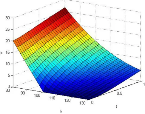
4.1.1
𝐶(𝐾, 𝑡)
From Theorem 1.2.1 (with no-zero interest rate 𝑟) and from (2.1) we obtain 𝐶(𝑡, 𝑆0, 𝐾) = e−𝑟𝑇𝐾1−𝑅𝑆𝑅 0 2𝜋 ∫ ℝ e−𝑖𝜉𝑙𝑜𝑔𝑆0𝐾−𝑇 𝜓(−(𝜉+𝑖𝑅)) (𝑖𝜉 − 𝑅)(1 + 𝑖𝜉 − 𝑅) (4.1) where 𝜓 is the characteristic exponent function (3.1)
𝜓(𝜉) =(− 𝐶 Γ(−𝑌 )[(𝑀 − 𝑖𝜉)𝑌 + (𝐺 + 𝑖𝜉)𝑌 − 𝑀𝑌 − 𝐺𝑌])
The choice of parameters (CGMY) is based on Carr, Peter, Geman, H´elyette, Madan, Dilip B., Yor, Marc (2002). ”The fine structure of asset returns: an empirical investigation”.
The interest rate 𝑟=0.05.
For the implementation we use MATLAB
%%%%%%%%%%%%%CGMY_call_option.m%%%%%%%%%%%%%% close all clear all % parametri % Y in [-inf,2] (interessante in [1,2]) % scelta 1 Y = 1.50683; C = 0.08; G = 25.04; M = 25.04; % R in [-G,M] R = 2; r = 0.05; S0 = 100; % tempi
4.1 Numerical evaluation: CGMY model 25 t = linspace(0,1,20); % strike k = linspace(85,135,20); % integrazione numerica lt = length(t); lk = length(k); V = zeros(lt,lk); for i=1:lt for j=1:lk V(i,j) = CGMY_value1(t(i),k(j),Y,C,G,M,R,r,S0); end end [K,T] = meshgrid(k,t); surf(K,T,Q) xlabel(’k’) ylabel(’t’) zlabel(’V’)
where the function value(𝑡(𝑖), 𝑘(𝑗), 𝑌, 𝐶, 𝐺, 𝑀, 𝑅, 𝑟, 𝑆0) is %%%%%%%%%%%%CGMY_value.m%%%%%%%%%%%%%
function [V] = CGMY_value1 (t,k,Y,C,G,M,R,r,S0)
% integrazione numerica
% estremi di integrazione a = -100000;
b = 100000;
26 4. Application
V = h*quad(@(u)CGMY_integrand1(u,t,k,C,G,M,Y,R,S0),a,b); end
where CGMY integrand1 is
%%%%%%%%CGMY_integrand1.m%%%%%%%%%%%%
function [y] = CGMY_integrand1 (u,t,k,C,G,M,Y,R,S0)
psi = CGMY_characteristic_exp1(+u-1i*R,C,G,M,Y);
y = exp(+1i.*u.*log(S0./k)-t.*psi)./((-1i.*u-R).*(1-1i.*u-R));
where characteristic exp1 is
%%%%%%%%CGMY_charcteristic_exp1.m%%%%%%%%%%
function [psi] = CGMY_characteristic_exp (u,C,G,M,Y)
4.1 Numerical evaluation: CGMY model 27
Figure 4.1: Call Price in the CGMY model
4.1.2
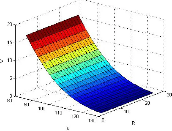
𝐶(𝐾, 𝑅)
With small changes in CGMY_call_option1.m we can see how, for fixed 𝑡, the price of an option changes with respect to the dampening coefficent 𝑅 and the Strike 𝐾.
%%%%%%%%%%%%%CGMY_call_option_R.m%%%%%%%%%%%%%% close all
clear all
% parametri
28 4. Application Y = 1.50683; C = 0.08; G = 25.04; M = 25.04; % interest rate r = 0.05; %tempo t = 0.5; S0 = 100; % coefficente di penalizzazione R = linspace(1.1,25,20); % strike k = linspace(85,130,20); % integrazione numerica lR = length(R); lk = length(k); V = zeros(lR,lk); for i=1:lR for j=1:lk V(i,j) = CGMY_value1(t,k(j),Y,C,G,M,R(i),r,S0); end end [K,RR] = meshgrid(k,R); surf(K,RR,V) xlabel(’k’) ylabel(’R’) zlabel(’V’)
4.2 Fourier transform valuation Vs Black-Sholes model 29
Figure 4.2: Call Price changes respect to 𝑅
4.2
Fourier transform valuation Vs Black-Sholes
model
In this section we want to see the difference between the valuation of the price of a call option using Black-Sholes formula and the valuation using Fourier transform method. With a little modification of our implementation we can see this difference.
First of all we change the characteristic_exp.m and we put inside the characteristic function of a normal distribution:
𝜑(𝑢; 𝜇, 𝜎2) = E[e𝑖𝑢𝒩 (𝜇,𝜎2)] = e𝑖𝜇𝑢−12𝜎 2𝑢2
30 4. Application
In Black-Sholes model 𝑆𝑇 = 𝑆0e𝑋𝑇 where 𝑋𝑇 ∼ 𝒩 ((𝑟 − 𝜎
2
2 )𝑡, 𝜎 2𝑡).
So the characteristic function becomes 𝜑𝐻𝑇(𝑢) = e −𝑡𝜓(𝑢) Where 𝜓(𝑢) = −𝑖𝑢(𝑟 − 𝜎 2 2 ) + 1 2𝜎 2𝑢2 (4.2) We choose 𝑟 = 0.05 & 𝜎 = 0.30 %%%%%%%%Characteristic _exp1.m%%%%%%%%%% function [psi] = characteristic_exp (u,r,d) psi = -1i*u.*(r-0.5*dˆ2)+0.5*dˆ2.*u.ˆ2;
4.2 Fourier transform valuation Vs Black-Sholes model 31
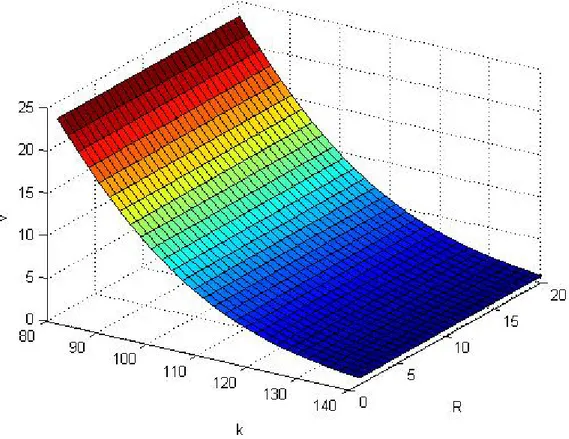
With the same changes made in 4.1.2 we can see how, for fixed 𝑡, the price of an option changes with respect to the dampening coefficent 𝑅 and the Strike 𝐾.
Figure 4.4: Call price with characteristic function of a normal distribution changes respect to 𝑅
32 4. Application
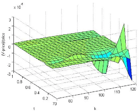
Finally we want to see the Approximation error between V (Price of an option with Fourier transform method) and price (Price of an option with Black-Sholes formula) :
𝑉 − 𝑝𝑟𝑖𝑐𝑒
𝑝𝑟𝑖𝑐𝑒 (4.3)
The value of a call option in terms of the Black-Scholes parameters is: 𝐶(𝑆, 𝑡) = 𝑆𝑁 (𝑑1) − 𝐾𝑒−𝑟(𝑡)𝑁 (𝑑2) 𝑑1 = ln(𝐾𝑆) + (𝑟 + 𝜎22)(𝑡) 𝜎√𝑡 𝑑2 = 𝑑1− 𝜎 √ 𝑡. where:
𝑁 () is the cumulative distribution function of the standard normal distribu-tion
𝑡 is the time to maturity
𝑆 is the spot price of the underlying asset 𝐾 is the strike price
𝑟 is the risk free rate (annual rate, expressed in terms of continuous com-pounding)
𝜎 is the volatility in the log-returns of the underlying.
So we modify Call_option.m in following way: %%%%%%%%%%call_option.m%%%%%%%%%%
close all clear all
% parametri r = 0.05;
4.2 Fourier transform valuation Vs Black-Sholes model 33 d = 0.3; % R coefficente di penalizzazione R = 2; S0 = 100; % tempi t = linspace(0.1,2,60); % strike k = linspace(70,110,51); % integrazione numerica lt = length(t); lk = length(k); V = zeros(lt,lk); d1 = zeros(lt,lk); d2 = zeros(lt,lk); price = zeros(lt,lk); for i=1:lt for j=1:lk V(i,j) = real(value(t(i),k(j),r,d,R,S0)); d1(i,j)=(log(S0./k(j))+(r+(dˆ2)/2).*(t(i)))/(d.*sqrt(t(i))); d2(i,j)=d1(i,j)-d.*sqrt(t(i)); price(i,j)=S0.*normcdf(d1(i,j))+ -k(j).*exp(-r*(t(i))).*normcdf(d2(i,j)); end end [K,T] = meshgrid(k,t); surf(K,T,(V-price)./price) xlabel(’k’) ylabel(’t’)
34 4. Application
zlabel(’(V-price)/price’)
Bibliography
[1] Carr, Peter, Geman, H´elyette, Madan, Dilip B., Yor, Marc (2002). The fine structure of asset returns: an empirical investigation. Journal of Business 75 (2): 305-332
[2] Deitmar, A. (2004). A First Course in Harmonic Analysis (2nd ed.).Springer.
[3] Eberlein, Glau and Papapantoleon Analysis of fourier transform valu-ation formulas and applicvalu-ations Applied Mathematical Finance Januar (2010).
[4] Katznelson, Y.(2004) An Introduction to Harmonic Analysis (Third ed.) Cambridge University Press.
[5] Pascucci, A.(2007) Calcolo Stocasstico per la Finanza Springer.
[6] Pini, B.(1977) Terzo Corso di Analisi Matematica, Cap. 1- Opera-tori lineari negli spazi ̷L𝑝 Cooperativa Libraria Universitaria Editrice
Bologna.
[7] Rudin, W.(1987) Real and Complex Analysis (Third ed.) McGraw-Hill. [8] Sato, K. (1999) L´evy Processes and Infinitely Divisible Distributions.
Cambridge University Press.
Ringraziamenti
Ringrazio il Relatore della mia tesi Prof.re Andrea Pascucci per i sugger-imenti, l’attenzione e la pazienza con cui ha seguito il mio lavoro.
Ringrazio inoltre la Prof.ssa Elena Loli Piccolomini per avermi guidato e aiutato nella parte della tesi riguardante la valutazione numerica, nonche l’ amico Michele Antonelli per gli utili suggerimenti sull’ uso di MATLAB.