Analysis of an innovative slim floor composite beam conformed by a custom GFRP pultruded profile and reinforced concrete.

(1)

ALMA MATER STUDIORUM - UNIVERSITÀ DI BOLOGNA

________________________________________________________________

SCUOLA DI INGEGNERIA E ARCHITETTURA

DICAM

Dipartimento di Ingegneria Civile, Ambientale e dei Materiali

International Master Course in Civil Engineering

FINAL DISSERTATION in

Structural Strengthening & Rehabilitation

Analysis of an innovative slim floor composite beam conformed

by a custom GFRP pultruded profile and reinforced concrete.

CANDIDATO: RELATORE:

Pedro Ospina Chiar.mo Prof. Andrea Benedetti

Anno Accademico 2012/2013

(2)

(3)

(4)

(5)

Acknowledgments

Among all the people that have contributed to my education as an engineer and, most importantly, as a human being, my loving family stands high above. Their unconditional support and teaching has paved this long and laborious road to my success and it is for this reason that they deserve this work entirely. Just to give them a piece of pride and a handful of joy, because nobody deserves it more than them.

(6)

(7)

Introduction

Italy, a country which has given birth to so many advances in engineering, has been the scenario for a vast number of constructions that have been left as record of its history, marking forever each overwhelming era. In recent history, the old quarters of many cities are still mostly made up of ancient houses which maintain functioning services. Just as humans, structures are troubled by the effects of time, where, subjected to constant loading, corrosion and accidental actions, its integrity and strength can’t be assured forever. Therefore, structural engineers have supplied themselves with the latest technology in materials and science to overcome this issues in the most efficient manner while portraying its historical significance.

Geographically trapped in a seismic region, these ancient constructions are constantly exposed to the lateral loading effects of earthquakes. One famous example is the small town of L’Aquila, which most of its historical center was seriously compromised and forced its inhabitants to evacuate their houses permanently. One of the possible solutions, for those allowed or worth the trouble, was to rehabilitate and strengthen the structures’ foundations, its brick walls and its wooden trussed beams. Even more, ancient military and bell towers, with slender structural configurations, absorbed intense seismic forces, resulting into a variety of longitudinal, transversal and diagonal cracks.

Over the last few decades, new materials such as Fiber Reinforced Polymers (FRP) have become the main solution for the strengthening of damaged structures. These materials are mainly used because of their extreme lightness, strength and ease of application. Carbon Fiber Reinforced Polymers (CFRP) have been widely used as an on-site intervention solution, with the scope of increasing the stiffness and ultimate strength of the remaining structural elements. Its excellent mechanical properties are counteracted by its high cost, specialized work force and low productivity; which has ultimately limited it versatility.

As a more monolithically structural element, pultruded profiles made from Glass Fiber Reinforced Polymers (GFRP) have been developed. Due to its process of fabrication, it has opened a door of unlimited possibilities by means of simple shape molding of the profile’s cross section, making its customization possible. Called a die, this heated mold joins the glass fibers from a roving and induces the curing of the polymer resin, maintaining the longitudinal direction of the fibers and the desired shape of the profile. As a continuum, this process creates

(11)

- 2 -

an infinitely long element with a constant cross section that allows the costumer to cut each element to the desired length. The pultrusion technology and its process, has allowed the material to be industrialized by producing structural profiles in marketable quantities at lower costs, thus becoming a competitive product. The mechanical behavior of pultruded elements are ruled by an orthotropic law of mechanics, making it perform differently in function of the direction of the load, and therefore, extra care is needed when using it for structural purposes.

Every structural material has been known to have its strengths and weaknesses. Where steel has great strength and stiffness, it has a high specific weight and is vulnerable to buckling and fire. Reinforced concrete elements are stocky and stiff with great resistance to fire but low strength and excessive volume that translates into weight. Finally, FRP has excellent strength, great stiffness, with extremely low specific weight but a brittle behavior and it is practically useless in case of fire. This has led to develop composite structural elements by joining structural profiles made from different materials and, ultimately, building an eclectic and efficient structural system.

For many years, steel-concrete composite structures have been used all over the world for building frames and limited span bridges. Its efficiency has been widely proven: each material strengthens the weakness of its counterpart providing the final structural product with stiffness, strength, stability, ductility and resistance to fire. Among the different composite profile configurations developed over the years, the Slimflor® system has portrayed an interesting solution, both in an engineering and an architectural point of view, by embedding the entire steel profile in the reinforced concrete. Following this principle, a composite structural element has been proposed, conformed of a customized GFRP pultruded profile and reinforced concrete, following the Slimflor® configuration and structural mechanism.

(12)

- 3 -

List of Symbols and Acronyms

FRP – Fiber reinforced polymer

GFRP – Glass fiber reinforced polymer

CFRP – Carbon fiber reinforced polymer

CLT – Classical laminate theory

FSDT – First-order shear deformation theory

ENA – Elastic neutral axis

PNA – Plastic neutral axis

SLS – Serviceability Limit State

ULS – Ultimate Limit State

ROM – Rule of Mixtures

FEM – Finite Element Method

𝐿_𝑐𝑏 – Length of the composite beam 𝑑𝑠𝑙𝑎𝑏 – Effective depth of the slab 𝑏_𝑤 – Web width of the composite beam 𝑏_{𝑠𝑙𝑎𝑏} – Width of the composite slab 𝐴𝑡𝑟 – Area of transversal reinforcement 𝜌_𝑡𝑟 – Transversal reinforcement ratio 𝑆_𝑖𝑗 – Stiffness of the lamina

𝑄𝑥, 𝑄𝑦, 𝑄𝑧 – First moment of area 𝐼_𝑥, 𝐼_𝑦, 𝐼_𝑧 – Second moment of area

𝐴_𝑐𝑏 – Total cross sectional area of the composite beam 𝐷_𝑠𝑐 – Dowel resistance of a stud

(13)

- 4 -

𝜏_𝑠𝑐 – Resistance of the shear stud shank

𝑓𝑐𝑘 – Characteristic compressive strength of concrete 𝑓_𝑐𝑑 – Design compressive strength of concrete 𝑓_𝑐𝑡 – Tensile strength of concrete

𝑓𝑐𝑡𝑚 – Means tensile strength of concrete 𝑓_𝑦𝑘 – Characteristic yield strength of steel 𝑓_𝑦𝑑 – Design yield strength of steel 𝛾_𝑐 – Reduction factor for concrete ν𝑥𝑦, ν𝑥𝑧, ν𝑦𝑧 – Poisson ratio E_𝑥, E_𝑦, E_𝑧 – Elastic modulus

E_𝑠, E_𝑐, E_𝑝, E_𝑓, E_𝑚 – Steel, concrete, FRP, fiber, matrix elastic modulus G𝑥𝑦, G𝑥𝑧, G𝑦𝑧 – Shear modulus

k – Shear deformation amplification factor

n – Modular ratio

V – FRP Composite total volume V_𝑚 – Matrix volume ratio

V_𝑓 – Fibers volume ratio

V𝑥𝑦, V𝑦𝑧, V𝑥𝑧 – Tangential shear force

σ𝑥, σ𝑦, σ𝑧 – Normal axial stress in the global axes σ1, σ2, σ3 – Normal axial stress in the local axes ε_𝑥, ε_𝑥, ε_𝑥 – Normal axial strain in the global axes ε1, ε2, ε3 – Normal axial strain in the local axes τ_𝑥𝑦, τ_𝑥𝑧, τ_𝑦𝑧 – Tangential shear stress

(14)

- 5 -

γ_𝑥𝑦, 𝛾_𝑥𝑧, γ_𝑦𝑧 – Tangential shear strain 𝜃𝑥𝑦 – Rotational strain due to torsion

𝛼 – Angle difference between the local and the global axes directions 𝜒_𝑥, 𝜒_𝑦, 𝜒_𝑧 – Curvature of the middle surface

𝑦_𝑘 – Distance to the k-th lamina 𝛿𝑦 – Deflection of the beam

(15)

- 6 -

Chapter 1: Fiber Reinforced Polymers

1.1 Literature Review

Fiber Reinforced Polymers (FRP) were developed at the mid of the 20th century in order to replace metallic materials, where the principle problem in Aerospace Engineering is gravity, these new materials provided the same strength and stiffness at a fraction of the weight. This materials (very similar to reinforced concrete) are formed of continuous aligned fibers embedded in a polymer matrix. The purpose of the matrix is to hold the fibers aligned in order to make them work as a whole, where fibers provide the great majority of the strength and stiffness, the matrix provides resistance to shear stresses. There exists a variety of fibers as well as a variety of matrices, being two the main branches: thermoset and thermoplastic polymers. Inside the thermoset branch, resins are the most widely used, presented as epoxy, phenolic and polyester. It is thanks to the vast options of fibers and polymer matrices that FRP is a highly efficient structural system designed to suit our problems accordingly.

Over the years, Carbon Fiber Reinforced Polymers (CFRP) and Glass Fiber Reinforced Polymers (GFRP) have grown to be the most widely used structural materials over many engineering fields. Starting in Aerospace Engineering and expanding to Mechanical Engineering, to finally introduce its versatility to Civil (Structural) Engineering. These last decades have been a preset for research and development, focusing its use on civil infrastructures strengthening. Currently, pultrusion technology is the most promising FRP structural system to compete with steel and reinforced concrete structures, especially for low height building frames and limited span bridges.

The pultrusion process is simple, efficient and maintains a high level of product quality, this last being crucial for the analysis and design of a structure which relies on its mechanical properties consistency. By means of a mechanical puller, placed at the end of the process, fiber rovings are submerged in a resin bath, guided and aligned to finally enter a heated die that both cures the resin and shapes (or molds) the structural element to the desired shape, exiting as a constant cross section element which is cut by a saw to the desired length. Besides the longitudinal (principal horizontal axis) rovings, a strand mat that surrounds the element is placed as shear reinforcement. The process can be appreciated at Figure 1.

(16)

- 7 -

Figure 1. Pultrusion production process and variety of profiles.

1.2 Mechanical Behavior

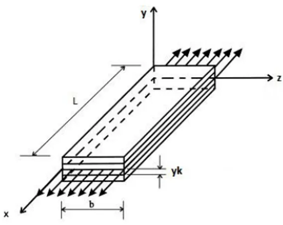
FRP has a particular mechanical behavior, where its properties are divided into two approaches: the micromechanical and the macromechanical level, being both approaches equally important in the understanding and the correct estimate of the resistance of its structural elements. From this point forward, the axes considered will be taken as seen in Figure 2.

Figure 2. Unidirectional laminate subjected to normal stress.

1.2.1 Micromechanical analysis

The micromechanical theory focuses on the interaction between individual fibers and the matrix surrounding them, where the main aspect is the adhesion at their interface, therefore, its main role is to assure a proper transfer of stresses from the matrix to the fibers. This approach is used for lamina design, it being a single row of fibers placed longitudinally and surrounded by a polymer matrix, forming a very thin plate. This is the simplest way of representation of an FRP and is the basis for the design of pultruded FRP elements, taking much attention to its orthotropic mechanical properties that come with it. By means of area ratios (percentage of the

(17)

- 8 -

total cross sectional area) between the fiber and the matrix, the elastic properties are calculated. Called the “Rule of Mixture”, the elastic modulus for each axis direction is given by:

𝐸_𝑥 = 𝐸_𝑓𝑉_𝑓+ 𝐸_𝑚𝑉_𝑚 (1.1) 𝐸_𝑧 = 𝐸𝑓𝐸𝑚 𝑉𝑚𝐸𝑓+𝑉𝑓𝐸𝑚 (1.2) ν_𝑥𝑧 = ν_𝑚V_𝑚+ ν_𝑓V_𝑓 (1.3) Where: 𝑉𝑓 =𝐴_𝐴𝑓 ; 𝑉𝑚 =𝐴_𝐴𝑚 (1.4)

A is the total area of the lamina’s cross section and the areas of each material inside the composite. The assumptions taken for this analysis to be real are: perfect bonding between the two materials, which permits to assume a uniform strain along the x-axis direction and uniform stress in the z-axis direction.

1.2.2 Macromechanical analysis 1.2.2.1 The lamina

1.2.2.1.1 Stress-strain relationship

Where an anisotropic material is considered to have a behavior which will vary depending on each possible vector of load application, there is coupling between all of its 36 constants which represent the membrane and bending deformations in each axis by influence of the external loads, keeping in mind that there are no planes of symmetry. The stress-strain relation of anisotropic materials can be represented by its mechanical relationship between the stresses, strains and its 36 independent constants:

(18)

- 9 - { 𝜎_𝑥 𝜎_𝑦 𝜎_𝑧 𝜏_𝑦𝑧 𝜏_𝑧𝑥 𝜏𝑥𝑦} = [ 𝑐₁₁ 𝑐₂₁ 𝑐₃₁ 𝑐₄₁ 𝑐₅₁ 𝑐₆₁ 𝑐₁₂ 𝑐₂₂ 𝑐₃₂ 𝑐₄₂ 𝑐₅₂ 𝑐₆₂ 𝑐₁₃ 𝑐₂₃ 𝑐₃₃ 𝑐₄₃ 𝑐₅₃ 𝑐₆₃ 𝑐₁₄ 𝑐₂₄ 𝑐₃₄ 𝑐₄₄ 𝑐₅₄ 𝑐₆₄ 𝑐15 𝑐25 𝑐35 𝑐45 𝑐55 𝑐65 𝑐16 𝑐26 𝑐36 𝑐46 𝑐56 𝑐66]{ 𝜀_𝑥 𝜀_𝑦 𝜀_𝑧 𝛾_𝑦𝑧 𝛾_𝑧𝑥 𝛾_𝑥𝑦} (2)

When dealing with two planes of symmetry with a third plane perpendicular to them, we can establish a reduced matrix with only 9 independent constants representing the stiffness of an orthotropic material: { 𝜎_𝑥 𝜎𝑦 𝜎𝑧 𝜏𝑦𝑧 𝜏𝑧𝑥 𝜏𝑥𝑦} = [ 𝑐₁₁ 𝑐₂₁ 𝑐₃₁ 0 0 0 𝑐12 𝑐22 𝑐32 0 0 0 𝑐₁₃ 𝑐₂₃ 𝑐₃₃ 0 0 0 0 0 0 𝑐₄₄ 0 0 0 0 0 0 𝑐₅₅ 0 0 0 0 0 0 𝑐₆₆]{ 𝜀_𝑥 𝜀𝑦 𝜀𝑧 𝛾𝑦𝑧 𝛾𝑧𝑥 𝛾𝑥𝑦} (3)

Introducing the engineering constants: the elastic modulus (E), shear modulus (G) and the Poisson ratio (ν) we obtain:

{ 𝜎_𝑥 𝜎_𝑦 𝜎_𝑧 𝜏_𝑦𝑧 𝜏_𝑧𝑥 𝜏𝑥𝑦} = [ 𝐸𝑥𝑥 −𝐸𝑦𝑦/ν𝑦𝑥 −𝐸𝑧𝑧/ν𝑧𝑥 0 0 0 −𝐸_𝑥𝑥/ν_𝑥𝑦 𝐸_𝑦𝑦 −𝐸_𝑧𝑧/ν_𝑧𝑥 0 0 0 −𝐸_𝑥𝑥/ν_𝑥𝑧 −𝐸_𝑦𝑦/ν_𝑦𝑧 𝐸_𝑧𝑧 0 0 0 0 0 0 𝐺_𝑥𝑥 0 0 0 0 0 0 𝐺_𝑦𝑦 0 0 0 0 0 0 𝐺_𝑧𝑧]{ 𝜀_𝑥 𝜀_𝑦 𝜀_𝑧 𝛾_𝑦𝑧 𝛾_𝑧𝑥 𝛾_𝑥𝑦} (3.1) Where: 𝐺𝑦𝑧 =_2(1+ν𝐸𝑦𝑦 𝑦𝑧) ; 𝐺𝑧𝑥 = 𝐸𝑧𝑧 2(1+ν𝑧𝑥) ; 𝐺𝑥𝑦 = 𝐸𝑥𝑥 2(1+ν𝑥𝑦) (4) ν_𝑦𝑧 = 𝜀𝑧 𝜀𝑦 ; ν𝑧𝑥 = 𝜀𝑥 𝜀𝑧 ; ν𝑥𝑦 = 𝜀𝑦 𝜀𝑥 (5)

(19)

- 10 -

For the case of a plate, the normal stress in the y-axis and shear stress resistance in the yz-plane and xy-plane can be neglected since they are considerably smaller compared to the ones in the xz-plane. With this in mind, we consider a lamina as a plate by setting the final matrix to describe its strength under plane stress, with 3 independent constants:

{ 𝜎_𝑥 𝜎_𝑧 𝜏_𝑥𝑧} = [ 𝐸_𝑥𝑥 −𝐸_𝑥𝑥/ν_𝑥𝑧 0 −𝐸𝑧𝑧/ν𝑧𝑥 𝐸_𝑧𝑧 0 0 0 𝐺_𝑥𝑧] { 𝜀_𝑥 𝜀_𝑧 𝛾_𝑥𝑧} (3.2)

To compare it with an isotropic material such as steel (with 2 independent constants), the matrix representation is: { 𝜎𝑥 𝜎𝑧 𝜏𝑥𝑧 } = [−𝐸𝐸_𝑥𝑥/ν_𝑥 0 −𝐸_𝑥/ν_𝑥 𝐸_𝑥 0 0 0 𝐺𝑥𝑧 ] { 𝜀𝑥 𝜀𝑧 𝛾_𝑥𝑧} (3.3)

1.2.2.2 Classical Laminate Theory

In order to determine the stiffness of the lamina, by means of classical laminate plate theory, the relationship between the materials deformations and the external loads applied to it. Paying attention that this theory establishes the axial strains according to the middle surface of the lamina and the shear strains are related to the extremes of the plate, forming the angles of curvature. As the name of the theory says, when considering the element as a plate, some degrees of freedom are not considered, them being: 𝜀_𝑦, 𝛾_𝑥𝑦, 𝛾_𝑦𝑧, 𝜒_𝑦. The reason for this assumption is done by reasoning that their values are significantly smaller compared to the main degrees of freedom, resulting into insignificant variations of the final results. The matrix representation of the lamina becomes:

(20)

- 11 - { 𝜀_𝑥 𝜀_𝑧 𝛾_𝑥𝑧 𝜒𝑥 𝜒𝑧 𝜃_𝑥𝑧} = [ 𝑎₁₁ 𝑎₃₁ 𝑎₅₁ 𝑏₁₁ 𝑏₃₁ 𝑏₅₁ 𝑎₁₃ 𝑎₃₃ 𝑎₅₃ 𝑏₁₃ 𝑏₃₃ 𝑏₅₃ 𝑎₁₅ 𝑎₃₅ 𝑎₅₅ 𝑏₁₅ 𝑏₃₅ 𝑏₅₅ 𝑏₁₁ 𝑏₃₁ 𝑏₅₁ 𝑑₁₁ 𝑑₃₁ 𝑑₅₁ 𝑏13 𝑏33 𝑏53 𝑑13 𝑑33 𝑑53 𝑏15 𝑏35 𝑏55 𝑑15 𝑑35 𝑑55]{ 𝑁_𝑥 𝑁_𝑧 𝑉_𝑥𝑧 𝑀𝑥 𝑀_𝑧 𝑇𝑥𝑧} (6)

Where the axial strain is the variation of deformation over its length in its own axis, the shear strain is due to the angle formed between the ratios of the variation of deformation in function of its perpendicular axis, rotating according to its middle surface. Where two shear strains exist in each plane, the final shear strain is the sum of these two angles. The curvature is the rotation of the middle surface due to the bending moment and the twist is the rotation due to an applied torque. The matrix of constants which does the coupling between the different loads actions have been divided into three sub matrices. The “a” matrix contains the shear-extension coupling coefficients, matrix “b” (symmetric) the bending-extension coupling coefficients and finally the “d” matrix the bend-twisting coupling coefficients. This approach is commonly known as the Kirchhoff-Love Plate theory.

1.2.2.3 First-order Shear Deformation Theory

Following the principles of Timoshenko and the original Reissner-Mindlin plate theory, the shear deformations can play a significant role due to the low shear stiffness modulus (G) that FRP materials have and, therefore, the missing factors for shear can be introduced by means of the first-order shear deformation theory (FSDT). This factors account for the two missing shear strains in equation (6) and can be represented in a separate matrix, allowing to have both CLT and FSDT as needed. This type of deformation is important when dealing with shear deformations in a beam, being bending moments and in-plane shear deformation much more crucial that out-of-plane deformations like warping (in the case of torque). Since it has been considered that CLT is an acceptable approach for practical purposes. The additional matrix is:

{_𝛾𝛾𝑦𝑧 𝑥𝑦} = [ ℎ₄₄ ℎ₆₄ ℎ₄₆ ℎ₆₆] { 𝑉_𝑧 𝑉𝑥} (6.1)

(21)

- 12 -

Called the transverse shear stiffness matrix, the “h” matrix is used when these two shear strains want to be accounted as part of the total deformation of the laminate. When summing up the contribution of each lamina, the “h” coefficients of the matrix are calculated by equation (8.3).

1.2.2.4 The laminate

The analysis of the laminate, it being the staking of various laminae (a sequence of laminas) and focusing on the mechanical contribution of each lamina to the laminate. This laminate, or even laminates, will eventually take the shape to become a pultruded element, where its resistance is calculated by means of these approach.

To counteract the orthotropic weakness behavior of each lamina, they are combined together at different angles to generate a final laminate that is able to withstand all type of stresses coming from external loading in its three main directions. The sequence of staking depends on the direction of the fibers, the symmetry and the balance of the laminae combination, as seen in Figure 3.

Figure 3. Laminae distribution of a multi-directional laminate.

To account for the contribution of each lamina to a laminate, as well as the contribution from each lamina, a transformation matrix is needed. By means of this matrix we can consider the local direction of each lamina and place its contribution to the global coordinates. By simple trigonometry, a relationship between the vector components in the local axis can be represented to the global axis and hence the transformation matrix is obtained. To avoid confusion, the global axis have been renamed, where the (x,y,z) used to represent the local axis of each lamina, it has been replaced by (1,2,3), and hence we get:

(22)

- 13 - { 𝜀₁ 𝜀₃ 𝛾13 } = [ 𝑐𝑜𝑠 2_𝛼 _𝑠𝑖𝑛2_𝛼 _{− 2 sin 𝛼 cos 𝛼} 𝑠𝑖𝑛2_𝛼 _𝑐𝑜𝑠2_𝛼 _{2 sin 𝛼 cos 𝛼}

sin 𝛼 cos 𝛼 −sin 𝛼 cos 𝛼 𝑐𝑜𝑠2_{𝛼 − 𝑠𝑖𝑛}2_𝛼 ] { 𝜀_𝑥 𝜀_𝑧 𝛾𝑥𝑧 } (7.1) {𝛾_𝛾23

12} = [ cos 𝛼 − sin 𝛼sin 𝛼 cos 𝛼 ] { 𝛾_𝑦𝑧

𝛾𝑥𝑦} (7.2)

To avoid incompatibility of deformations, involving fracture mechanics, the bonding between laminae must be considered as perfect. With this as a starting point, we can simply sum the stiffness (S) contribution of the k-th lamina to the total stiffness matrix [𝑎 𝑏

𝑏 𝑑] and we can get a global matrix system that represents the laminate’s stiffness. To do so we use the equations:

𝑎_𝑖𝑗 = ∑𝑁 ( 𝑘=1 𝑆𝑖𝑗)𝑘(𝑦𝑘− 𝑦𝑘−1) (8.1) 𝑏_𝑖𝑗 =1₂ ∑𝑁 ( 𝑘=1 𝑆𝑖𝑗)𝑘(𝑦𝑘2− 𝑦𝑘−12 ) (8.2) 𝑑_𝑖𝑗 =1₃ ∑𝑁 ( 𝑘=1 𝑆𝑖𝑗)𝑘(𝑦𝑘3− 𝑦𝑘−13 ) (8.3) ℎ_𝑖𝑗 =5₄ ∑𝑁 ( 𝑘=1 𝑆𝑖𝑗∗)𝑘[𝑡𝑘−_𝑡42(𝑡𝑘𝑦𝑘2 − 𝑡_𝑘3 12)] (8.4)

This final step allows the acquisition of the laminate’s stiffness in its global reference axes, which in turn becomes the beam element as a whole, therefore, we can calculate its resistance under different types of loading; just as beams for building frames. Essentially, suppliers of FRP pultruded profiles give an extensive quantity of strength and resistance properties that permit engineers to calculate the required sizing of beam members. This data can be appreciated at the documents located at the Annex.

(23)

- 14 -

1.3 Pultruded GFRP cross sections

1.3.1 Mechanical and general properties

The combination of fiber and matrix type permits to design an FRP element with a vast range of possibilities, permitting to control the level of stiffness, strength, ductility, corrosion resistance, fire resistance, etc. Needless to say, the higher the mechanical properties of the material, the higher the costs. For example, GFRP elements range their elastic modulus values between 20 and 30 [GPa], making it very compatible to concrete which has a very similar range of stiffness values. As for the strength, it is unfortunate that its behavior is brittle, which is highly undesired because of its unexpected failure. Nevertheless, the strength values range between 250 and 350 [MPa] which is comparable to the strength of steel. As for the specific weight of this material, the ranging values go from 16 to 19 [kN/m3] which is up to seven times lighter than steel and around 50% lighter than reinforced concrete, making the montage quite easy.

The weakest link of this type of members is its resistance to fire, where a diversity of polymeric coatings can reduce the flammability and smoke generation, it doesn’t change the effect of temperature to the matrix, which basically turns it useless after 350 degrees Celsius and a reduction of strength of about 50% after only 250 degrees Celsius. The problem arises from the glass transition temperature of the matrix resin, where, once it is reached, the material is decomposed. This leaves the fibers working independently, leading to a progressive failure up to the total failure of the element.

Fortunately, besides the vulnerability of glass fibers to water absorption, the corrosion resistance of these pultruded elements are excellent thanks to the polymer’s capabilities to enclose the fibers by not permitting water and other chemicals to degrade the material. This is the reason why it has become highly attractive in the use of bridge girders.

1.3.2 Normal stresses

Over the last decades, a variety of companies have developed an industrialized market that provides pultruded elements made from GFRP with an enormous supply and variety of geometrical profiles, mechanical properties, length, etc. In addition, some companies even provide services for the development of personalized cross sections, fitted to the design and desire of the costumer. Each company has accompanied its technology with deep research and testing over their products, in order to assure their mechanical behavior to costumers, up to the point of providing design codes and handbooks. The most common cross sections are the ones

(24)

- 15 -

commonly used in structural steel, such as I and H-shaped, as well as rectangular and circular hollow tubes, up to the point of hollow sandwich deck slabs. Even through the pultrusion process is not based on joining of separate laminas (to form a laminate), its behavior is analyzed as such. The variety of profiles offered by Creative Pultrusions can be seen at the Annex.

For the case of pultruded structural elements, we can pass from the analysis of a laminate to the simplified theory of resistance of materials; widely used for structural steel and reinforced concrete beam elements. Using the equation of curvature and the relationship that it has to normal strains:

𝜒𝑧 =_𝐸𝑀𝑧

𝑥 𝐼𝑧 (9)

𝜀_𝑥 = 𝜒_𝑧 𝑦 (10)

Being (M) the bending moment, (y) the distance from the neutral axis to the desired point of analysis and (I) the second moment of area (commonly known as moment of inertia). Equaling these two equations we can get the normal stresses present in each point along the height of the beam:

𝜎_𝑥 =𝑀𝑧 .𝑦

𝐼𝑧 [𝑀𝑃𝑎] (11)

The complexity of the material can make differences in resistance not only for each varying axes but also for the direction of application of the load, meaning that it behaves differently under tensile and compressive stresses. For example, Creative Pultrusions indicate a 10% increase of strength for compressive normal axial stress compared to tensile normal axial stress.

When dealing with the design values of its resistance, some manufactures and general building codes have reduced its characteristic bending moment resistance by 50% but in some cases, such as in deck systems, a reduction factor of 8 is used.

(25)

- 16 -

1.3.3 Shear stresses

For the case of shear stresses in the cross section, the equation presented by Zhuravskii, where (V) is the vertical shear, (Q) is the first moment of area and (b) the width of the cross section:

𝜏𝑦𝑧 = 𝑉_𝐼𝑦 𝑄𝑧

𝑧 𝑏𝑤 [𝑀𝑃𝑎] (12)

In a general case, thin walled cross section beams such as I-beams have the majority of their shear stress concentrated in the web, where its maximum is located at the centroid of the cross section.

The resulting stress from this equation is equal for both the vertical (yz-plane) and the horizontal (xz-plane or longitudinal) shear stress since it must be fulfilled for equilibrium. When analyzing such shear stresses in the longitudinal direction we can find the weakest point of a pultruded beam, since its strength only depends on the strength of the matrix between the lines parallel to the fibers. To counteract this weakness, production companies have included a strand mat of discontinuous fibers that surrounds the longitudinal section to form a 45 degree reinforcement.

The materials sensibility and weakness to shear stress, due to the matrix and not to the fibers, has obliged design guides and codes (either made by manufacturing companies or by government institutions) to reduce its resistance by a factor of 3. For the case of pultruded decks, a massive 75% decrease is introduced, or in other words, the design shear resistance of a pultruded element is one fourth of the calculated resistance value.

1.3.4 Deflection

When analyzing the deflection of pultruded beams, flexure beam theory of Euler-Bernoulli is no longer applicable due to the sensitivity of the material to shear deformations. These characteristics coming from shear strains have demonstrated to contribute considerably to the beam’s deflection. Therefore, Timoshenko’s flexure beam theory is needed to account this effect. The first theory establishes that the angle of rotation of the beam (the first derivative of the deflection function) is equal to the curvature of the cross section (the inverse of the radius of curvature), where Timoshenko’s theory establishes that these two angles are not equal, and

(26)

- 17 -

thus generating a total deflection from the bending moment alone plus a shear deformation. The beam’s differential equation under a distributed load (q) becomes:

𝑞(𝑥) = 𝐸𝑥 𝐼𝑧(𝑑 4_𝑦 𝑑𝑥4+ 1 𝑘 𝐴𝑐𝑏 𝐺𝑥𝑦 𝑑2𝑞 𝑑𝑥2) (13)

The shear coefficient (k), defined as an incremental factor that is the ratio of the maximum shear stress divided by the mean shear stress in the cross section, can also be calculated by 𝑘 = 10(1 + ν) 12 + 11ν⁄ (Eq.14) for a rectangular solid cross section. Solving the differential equation with the proper boundary conditions with fixed end supports, the deflection equation was obtained and used to calculate its maximum, located at mid-span of the beam:

𝛿_{𝑦,𝑚𝑎𝑥} =𝑞𝐿𝑐𝑏2 8 ( 𝐿2𝑐𝑏 48 𝐸𝑥𝐼𝑧+ 1 𝑘 𝐴𝑐𝑏𝐺𝑥𝑦) (15)

Consider the discrepancy between this calculation and the one used by CLT, which in reality uses the same assumptions as Euler-Bernoulli beam criteria and hence, the use of FSDT is once again needed to keep consistency in the analysis.

1.3.5 Connection

There are two types of connections for pultruded elements: a bonded connection by means of an adhesive, a bolted connection with supporting pressure plates or a mixture of the two. Adhesive joints have been proven to have great resistance but of catastrophic sudden failure, which sets engineers into a doubtful thinking. Even though the bonded connection can withstand higher loads than the bolted one, its failure happens in the element and not in the connection; where fracture happens due to shear stresses in the element’s layer (thinking of it as the separation between laminas) close to the adhesive. Therefore, the strength of the bonded joint actually depends on the interlaminar shear strength of the GFRP pultruded material.

Bolted connections follow the same type of failure as the one seen in bolted connection analysis for steel profiles, with the difference that the orthotropic characteristics of the material make it more complex to analyze. The principal failure types that need to be calculated to assure the

(27)

- 18 -

proper resistance of the connection, and the weakest link of these five possible failures becomes the leading resistance value of the bolted connection:

- Shear failure due to tension, characterized by a perpendicular line passing through the hole.

- Cleavage or splitting of the extremity, occurring parallel or perpendicular to the line of loading.

- Bearing failure due to compressive stress concentration.

- Shear-out failure that follows the line of the hole up to the border of the element. - Shear failure of the bolt, which can be either made of steel or even of FRP material.

Pultruded GFRP structural elements have proven to have excellent mechanical characteristics, some considerable weaknesses and great manageability (thanks to its very low specific weight), but a reduced experience of its use and real life testing (specially for long-term behavior) has introduced uncertainty in engineers criteria, leading them to punish its strength with massive reduction factors.

1.4 Composite steel-concrete structural elements

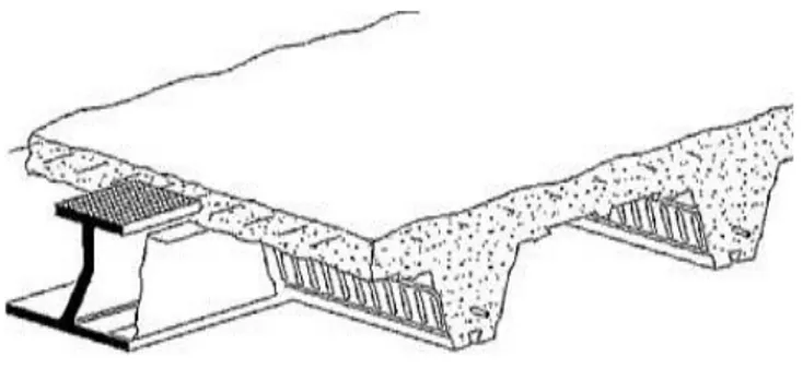
The use of composite structures have been developed with great success as an efficient system, permitting building frames to be light, cover long spans and increase construction productivity. Among a diversity of different steel-concrete composite systems, the Slimflor® beam system has proven to solve not only the basic problems in structural engineering but also increase the fire resistance of the structure, as well as becoming more architecturally appealing. Figure 4 gives a good representation of the final product and its conforming parts.

(28)

- 19 -

The procedure to its construction consists on the placement of the steel beam, called an asymmetric beam due to the difference of size of the flanges’ width. Once the beam has been joined properly to the column through a welded or bolted connection, the steel deck can be placed on top of the lower flange, transversal to the beam’s axis. The upper steel grid reinforcement is placed and, finally, the concrete is poured. Once the concrete has hardened, the composite beam element is conformed according to the design and it can perform its job accordingly.

1.4.1 Cross section analysis

When analyzing the behavior of a composite beam a variety of factors must be taken into account, such as: the end support, its performance for negative and positive bending moment, its behavior at the elastic phase as well as for the plastic one. Even more importantly, the composite behavior between the two materials depend of their slipping interaction, which turns it into a key factor. Meaning that, to assure the composite monolithic behavior of the structural element, a proper shear connection must exist between them, otherwise, its real behavior will be very different.

1.4.1.1 Neutral axis

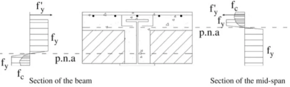
For the case of a beam with fixed supports, the inversion of flexural stresses make the beam perform in very different ways, where for positive bending moment (sagging) the lower flange is in tension, the concrete, the upper steel beam’s flange and the steel reinforcement are working in compression. For negative bending moment (hogging), the lower flange must work in compression with some support from the concrete surrounding the web, these being equilibrated by the top reinforcement and the upper flange of the steel beam (both working in tension). Design guides recommend that the tensile resistance of concrete must be neglected for Ultimate Limit State analysis. Figure 5 shows the location of the two plastic neutral axis in that particular beam since it changes depending on the beam’s characteristics.

Considering all of the previously mentioned facts, this type of composite beam has three different neutral axes:

- The elastic neutral axis (ENA) used for Serviceability Limit State (SLS) verifications, set at the centroid of the composite beam’s cross section can be calculated by means of area distribution by reaching an equivalent modulated area. This approach homogenizes the cross section as if it was conformed of one single material by means of increasing

(29)

- 20 -

the area of the steel elements so to develop the same resistance as if it was made of concrete. This modular ratio is obtained by dividing the materials’ elastic moduli:

𝑛 = 𝐸𝑠

𝐸𝑐 (16)

- The plastic neutral axis (PNA-) for hogging bending moment (negative bending moment set at the supports) which is obtained by finding an equilibrium point between the ultimate compressive and tensional forces that provide each material.

- The plastic neutral axis (PNA+) for sagging bending moment (positive bending moment with its maximum at mid-span) it is determined in the same manner as for hogging bending moment but with the stresses inversed and considering the changes resulting from the cracked concrete when it is neglected.

Usually, the PNA(+) is placed at the slab’s height of the T-shaped composite beam and the PNA(-) at mid-height of the web. Certainly, the placing of these axes depend on a variety of reasons, but principally on geometric and mechanical properties of the cross section and the materials, respectively. The importance of these factors is high since they are the base for all the continuing calculations which are dealt with next.

1.4.1.2 Shear interaction

The efficiency of these composite system depends on the shear interaction that both materials have to assure that they are working together, especially considering the fact that, being materials with very different stiffness and strength values, their deformations diversify, resulting in a slip between the two elements. For the Slimflor® system, there is contact shear interaction (along the web’s and top flange’s perimeter) with a mean value of 0.6 [MPa] according to [4], but in the case of a needed increase in shear interaction, vertical shear studs can be welded on top of the steel beam’s top flange or elsewhere. For this purpose, three scenarios are present in any given section:

- Full shear interaction: the whole composite beam works together harmonically as if it was a single homogeneous cross section with a single curvature angle.

- Partial shear interaction: both materials work together with a limited slip that establishes a curvature to each cross section but sharing some of the total deformation. In other words, creating a jointed single second moment of area (inertia) but having

(30)

- 21 -

different curvatures. It has been proven that, the loss of shear interaction due to slip, projects into small losses in resistant bending moment.

- No shear interaction: Each material element works independently, having independent curvatures. This system is not possible in reality unless oil or frictionless materials are used at the interface.

When shear studs are present, either on the top flange or in the web, they are resisted by the dowel action resulting from the concrete surrounding it. Obtained as an empirical equation from push-out tests, [3] has estimated the maximum dowel resistance of a single shear stud. Another check must be done to assure that the failure doesn’t come from the shearing of the steel rebar. Therefore, the minimum of the two will lead the design:

𝐷_{𝑠𝑐,𝑚𝑎𝑥} = 0.5 𝐴_𝑠ℎ √𝑓𝑐𝑑 𝐸𝑐 (17.1)

𝜏_{𝑠𝑐,𝑚𝑎𝑥} = 0.8 𝐴_𝑠ℎ 𝑓_𝑢 (17.2)

1.4.1.3 Resistant bending moment

Once the PNA is known, by equilibrium to rotation, the ultimate resistant bending moment of the composite beam can be estimated. Needless to say, separate calculations must be performed for hogging and sagging resistant bending moment, taking into consideration the use of the proper PNA. Figure 5 shows the stress block distribution of the materials at its ultimate (plastic) state, where the concrete’s parabolic representation is simplified by a reduced rectangular one.

(31)

- 22 -

1.4.1.4 Resistant shear force

The resistance of the composite beam to shear stress has been simplified by only considering the contribution of the steel beam, and not only that but considering only the contribution of the web. By means of this approach, a big safety margin is achieved, which is highly desirable since shear failure can occur suddenly and in a brittle manner. Some authors have considered possible the contribution of the concrete trapped between the flanges, which, in the case of negative bending moment, not only it is partly in compression but also confined. Some authors and codes consider it to be too unreliable and prefer to focus on the steel section only.

1.4.1.5 Transverse resistance

In the transverse direction (yz-plane), the beam section that conform the composite slab, are part of the T-shaped composite beam’s flange, which is submitted to a hogging bending moment. This hogging bending moment is resisted by the slab’s transverse shear reinforcement that comes from the reinforcing grid. Equally, the vertical shear resistance of the slab must be verified, considering that it’s a resistant element without shear reinforcement. From Eurocode 2, the vertical shear resistance is given by:

𝑉_𝑅𝑑 = [0.18 (1 + √_𝑑200

𝑠𝑙𝑎𝑏) (100 𝜌𝑡𝑟 𝑓𝑐𝑘)

1/3_]𝑏𝑠𝑙𝑎𝑏 𝑑𝑠𝑙𝑎𝑏

𝛾𝑐 (18)

Where (𝑑_{𝑠𝑙𝑎𝑏}) is the effective depth of the slab, (𝜌_𝑡𝑟) the flexural reinforcement ratio and (𝑏_{𝑠𝑙𝑎𝑏}) the width, which is taken as 1 meter. The safety factor 𝛾_𝑐 has a given value of 1.5. As for other shear resistance verification, the composite T-beam’s flange must be checked for transverse resistance (in the xy-plane), specially for the fact that its thickness (the slabs thickness) can be quite low, ranging from around 80 to 100 [mm]. The shear strength verification in the slab is its resistance to longitudinal axial stresses resulting from the bending moment in the yz-plane, where the composite beam’s web joins the flanges. To calculate this resistance, [3] has given the equation:

(32)

- 23 -

Where the first term is the contribution of concrete to shear, the second is the dowel action contribution of the slab’s flexural reinforcement and the third is the friction contribution due to the compressive stress (𝜎_𝑧) chord in the slab which comes from the bending moment in the transverse direction. This stress has a compressive value and placed at the lower part of the slab/T-beam flange.

(33)

- 24 -

Chapter 2: The GFRP-RC Composite beam

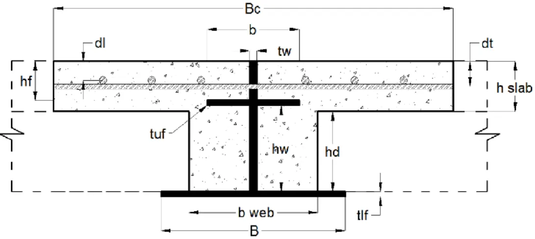
The complete analysis of the proposed beam has been done by comparing the results between a Finite Element Method model (FEM) and simple hand calculations done in an Excel spreadsheet. The objective of this is to understand how reliable hand calculations can be and, therefore, possibly use them as a reliable tool for future designs. Figure 6 shows the representation of the proposed GFRP-RC composite beam and the given name to each geometric property, which follows as well for the Excel calculation program. First, the Excel program will be dealt with in order to calculate a diversity of parameters and mechanical effects. Keeping in mind that the only one which depends entirely on the FEM simulation is the fire situation due to its time-step variable. However, some tools can help predict the resulting effect of fire after a 60 minute exposure.

2.1 Description of the element

The proposed composite beam has been formed from a base of a customized pultruded GFRP beam formed of an asymmetric I-beam with a continuous shear connector composed of a vertical extension of the web. For sake of simplicity, this extension of the web (hf) will be referred as “the fin” by analogy of a fish, and the final composite beam will be referred as GFRP-RC beam. The top extreme of the fin will give the total height of the GFRP-RC beam, and hence, the slab. To support the transversal steel bars, U-shaped milling or perforated holes can be performed on the fin. The grid reinforcement will consist of transversal steel bars and, supported over these, the longitudinal steel bars.

(34)

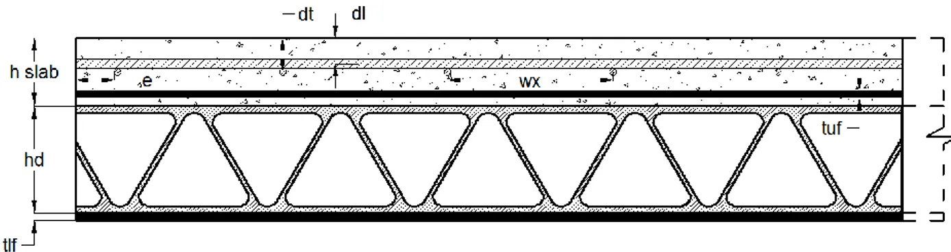
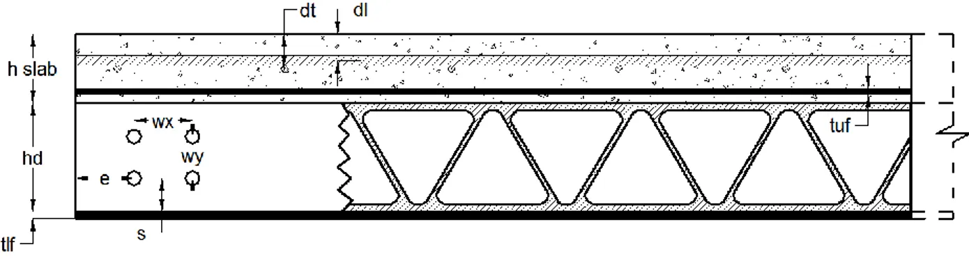
- 25 -

For the structural analysis, this is the GFRP-RC beam’s configuration but the reality of its shape is obtained when a GFRP pultruded deck is placed over the lower flange of the GFRP pultruded beam, which latter will be part of the composite slab. This matter will be dealt with on the next chapters but it’s important to keep it in mind to understand the construction process that makes this final composite beam possible.

The type of end support has been considered as fixed-fixed by following the research done by [55]. For hand calculations (Excel), supposing that each space of the cross section at the support connection has no rotation is not real, starting with the fact that the GFRP profile, having a bolted connection in its web and no connection to its flanges, in reality is working as a simply supported structural element. The concrete and steel reinforcement may be considered as part of a fixed connection, but being submitted to a negative bending moment (tensile axial stresses at the top of the beam), makes it quite complex to estimate its real behavior. Therefore, the only part that makes this system work as a fixed system is the longitudinal reinforcement.

Focused in the analysis of the lower bound potential resistance of the proposed composite FRP-RC beam, common pultruded profiles where chosen (from Creative Pultrusions company) and concrete of the lowest acceptable strength, 𝑓𝑐𝑘 = 20 [𝑀𝑃𝑎]. The chosen values for the geometric dimensions were chosen according to common limiting distances seen of slim floor examples presented at [4]. Refer to the Annex for the complete data used in the analysis as well as the material data provided by the manufactures of the GFRP pultruded profiles.

2.2 Analysis of the GFRP-RC beam

2.2.1 Material properties

Considering that the GFRP-RC composite beam has three different materials, the ROM approach was used to determine a unique elastic modulus and its mechanical properties. To do so, equations (1.1), (1.2) and (1.3) where used.

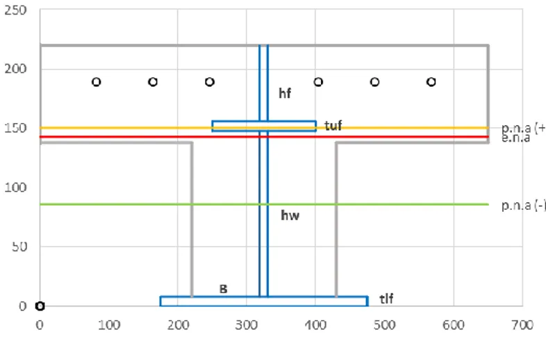
2.2.2 Determination of the neutral axis

As mentioned in the literature introduction, the neutral axes of a slim floor composite beam are three. There is one elastic neutral axis and two plastic ones as presented in Figure 7, where the two plastic neutral axes vary for the hogging and sagging bending moment. They are different due to the assumption that the tensile contribution of concrete is zero and only for sagging bending moment the compressive concrete was accounted. For the hogging bending moment, the compressive concrete trapped between the flanges is not accounted. For sake of simplicity, they have been named as PNA(+) and PNA(-) which clearly refers to the sign of the bending

(35)

- 26 -

moment at which the beam is subjected to. After obtaining these three axes, we can proceed to the calculation of the beam’s mechanical properties for each neutral axes, such as the first and second moment of area and the radius of gyration. It is interesting to notice how close together the PNA(+) and the ENA are, which, in raw words, can be said that the cross section has a “constant” behavior from zero loading up to failure for sagging bending moment. For the analysis of the ENA, the uncracked cross section is considered, which makes a difference in the calculation of the second moment of area.

It is very important to consider that this approach can drastically change if the neutral axes fall into places different to the ones seen in Figure 7, where, if the ENA is placed on the web or the PNA(-) at the flange, will represent unreal results. As an assumption, due to generally seen results, the neutral axes have been expected to been placed at each ranged zone. In other words, the use of these beams for other purposes other than the ones explained, is outside the scope of this thesis.

Figure 7. Placing of the neutral axes in the GFRP-RC composite beam.

2.2.3 Loading actions considered

Following the code’s loading principles, they were estimated for the analysis of the beam. Starting with the permanent actions of the different parts that conform the GFRP-RC composite beam, it was appreciated that the weight of the GFRP pultruded profile is extremely low with just 0.18 [kN/m2_{]. To account for a variety of possible permanent loads such as the gypsum}

board (dealt with later) and miscellaneous, a 0.5 [kN/m2_{] was given. For the variable actions,}

(36)

- 27 -

contributory symmetric length was placed equal to 5 meters. This length will be the same for the composite slab’s beam analyzed latter. This analysis can be appreciated at the Excel spreadsheet located in the Annex.

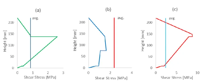
2.2.4 Shear stress distribution at the cross section

Using Equation (12) the shear stress distribution over the cross section was estimated, with an expected maximum at the point where the flange and the web meet since it represents a point for concentration of stresses. By looking at Figure 8, the difference between the average shear stress (the vertical line) over the cross section and the maximum are very different, resulting into incremental values of shear deformation. This ratio gives the value of the constant k, applicable in Equation (15) so to determine the maximum deflection. Since the three axes are placed at different parts of the beam, it can be seen how their maximum values can drastically change. This effect is seen especially at the ULS phase where the plastic neutral axes are very different among each other. As the figures show, the shear stress for the case of sagging bending moment is much higher than for the hogging case.

Figure 8. Shear stress flow. (a) Elastic phase, (b) Hogging bending moment plastic phase, (c) Sagging bending moment plastic phase.

2.2.5 Serviceability Limit State

The loading value for this verification came from the sum of the permanent and variable actions without any incremental factors. Bending moment and deflection values were calculated, considering the contribution from shear deformation. Even though this problem is applicable

(37)

- 28 -

for GFRP, for sake of safety, it has been applied to the GFRP-RC composite beam too. The value of the bending moment at mid-span for a fixed beam and double its value for the end supports (with a changed sign):

𝑀_𝑠𝑑(+) =𝑞𝑆𝐿𝑆 𝐿𝑐𝑏2

24 (20)

Using equations (9), (10) and (11), the normal axial stresses along the height of the beam where calculated, checking the values for the three different materials at their respective distances from the neutral axes. Applying this approach, the stresses in every point for each material (GFRP, concrete, steel) was calculated accordingly. For the case of sagging bending moment, the GFRP, the concrete and the reinforcement steel are submitted to lower values of axial stress than the ones allowed by the SLS. A problem arises when we verify the values obtained at the hogging bending moment since the concrete in compression (at the lower part) is well beyond the limiting values. However, this issue can be discarded considering that this contribution of concrete wasn’t accounted from the start, and thus, the resistant bending moment of the composite beam doesn’t suffer at all. Though, it must be kept in mind that this might bring excessive cracking and unacceptable aesthetic issues.

Maintaining constant the geometrical dimensions of the cross section (as previously stated) and changing only the span length, values for Graph 1 were generated. This will help understand the scope of possible use of this particular GFRP-RC beam in function of the maximum deflection at its mid-span. The horizontal dotted lines represent the limit that the code has considered as safe, and therefore, the beam remains inside the SLS limits even to spans longer than 8 meters. For the case of the analyzed beam, the six meter length span is by far inside the safe side.

Another check done was that of the vibrating behavior of the structural element, which has been introduced by the codes in order to assure a pleasurable function of the floor to people. Infrequent cycles per second of oscillatory motion could turn into perceivable vibrations, becoming an uncomfortable situation for its users. The result obtained at the analysis is well above the minimum value of 4 [Hz] cycles/second set by the code.

(38)

- 29 -

2.2.6 Ultimate limit state

The value of the distributed load for ULS received and increment of 35% for permanent loads and a 50% increment for variable loads. Following the assumptions of the code, the cross section was considered as fully plastic (elastic, perfectly plastic materials) with stress block representation of its components and the tension resistance of concrete was neglected.

It should be pointed out the changes that go through the section when it passes form the elastic (uncracked) phase to the plastic phase. The cracking of the element and the distribution of the stresses (due to the change in the neutral axes) will also change the second moment of area of the element and hence, a new one is generated. This new plastic second moment of area is calculated in the same manner as for the elastic one, where a modulated area approach is used, so to account for the proportional provision of each material, keeping in mind the particular situation of concrete, since it is the only one neglected once it has cracked. Both the GFRP and the steel reinforcement keep their original volumes and characteristics all the way from the elastic phase up to failure.

2.2.6.1 Resistant bending moment

For the hogging bending moment, the contribution of concrete in compression was completely unaccounted as done by [49], making the steel reinforcement bars and the GFRP profile equilibrate all of the forces present in the beam. This was decided due to the connection type with the column, where being (the concrete in compression) discontinuous at this point, the compressive contribution cannot be guaranteed. Only in the case of a concrete or a tube-shaped column there could be some proper interaction, however, for the purpose of this structural system, it is much more likely to be a slender column made of a steel or GFRP profile. Introducing a safety factor that accounts only the 85% of the resistance, the design resistant bending moment was obtained. Interestingly, the resistance for sagging bending moment, besides having the compressive contribution of concrete, it is lightly larger than the resistance for case of hogging bending moment.

2.2.6.2 Shear resistances

For all the different shear stress planes, there have been a variety of verifications that will help us assure that the beam can work properly. This becomes of major importance since it is the weak point of FRP pultruded elements. Among these shear stresses, there are:

(39)

- 30 -

- Longitudinal shear stress in the xz-plane in the elastic phase and plastic phase in the case of sagging bending moment, considering that their neutral axes are very close to each other.

- Longitudinal shear stress at the critical yz-plane in the plastic phase, being the point where the slab joins the web of the GFRP-RC beam.

- Vertical shear stress in the yz-plane in the plastic phase at the critical point where the slab joins the GFRP-RC web.

- Longitudinal shear stress in the xy-plane for the transverse reinforcement at the face of the fin.

Following the principle established by [3] and the code, the resistance to vertical shear in the yz-plane was taken into account only from the vertical elements of the pultruded beam (the web and the fin). Even if some authors consider a possible contribution from the concrete trapped between the flanges, it was decided not to count on it. Besides, the Pultex Design Manual has a very high penalization factor for the resistance to shear, with a reduction of 3 times its characteristic resistance. Even so, the element’s web is able to withstand the required shear force coming from the external loads.

(40)

- 31 -

The three main cases of shear stress planes are represented in Figure 9, where all three must be checked with care, otherwise, the beam can fail in unexpected manners with very dangerous consequences.

2.2.6.3 Shear interaction

For the shear interaction between the GFRP and the reinforced concrete, the section was considered as a homogeneous element, therefore, accounting that it has a full shear interaction. This approach is not only seen at steel-concrete composite slim floor design, but further studying of these effect is presented latter to assure the mentioned assumption. To assure even further the interaction, some particular elements can be considered as contributors. In the case of the GFRP-RC composite beam, some of them are from mechanical characteristics or contact friction between their interfaces. In this particular case of beam, some of the possible contributions are:

- The perimeter of the pultruded beam in contact with the concrete has a friction resistance which may be highly increased by adding an adhesive coating to the pultruded profile. The thesis done by [58] has concluded that a minimum contact shear resistance of 1 [MPa] can be guaranteed when an adhesive coating is used on the walls of the FRP element right before the pouring of the concrete. Besides, the failure happens at the unconfined concrete interface and not at the adhesive.

- The fin, together with the transverse reinforcement, form a shear stud-like mechanical system. The advantage of this factor is that it is continuous, leaving no concentration of stresses as happens on the dowel action in steel studs. It must be taken with care the effect and resistance of the transverse reinforcement, because an excessive number of perforations can weaken the material critically.

- The bolts from the connection of the pultruded profile, with its horizontal configuration, can work as shear studs. Since these bolts will be embedded in the concrete, a possible way to exploit them is by stretching the head of the bolts to form a stud-like mechanical system. This way the beam section can have horizontal shear connectors that contribute in the critical shear zone, exactly where they are needed the most. Fortunately, the resistance of the FRP web to longitudinal shear is higher than for vertical shear (due to the direction of the fibers) and therefore, if it can withstand the forces from the vertical shear, it can easily withstand the longitudinal forces as well. Certainly, it is wise to verify that it is so.

(41)

- 32 -

2.2.6.4 Slip

With the assumption of full shear interaction, the slip between the two members is zero. This assumption can be taken with more certainty than in the case of the steel-concrete composite beam since, the reason of the slipping is partly due to the big difference of stiffness among the two materials. For the GFRP-RC beam, the elastic moduli differences is very small, making the deflections of the two much more compatible, therefore, making slip values smaller. The research done by [55] has shown than the values of slip between the steel beam and the surrounding concrete of the slim floor was practically nonexistent.

For the case of the program, a rough calculation was performed to estimate a possible value of slipping that can permit to know (as a secondary approach) the required strength of the shear connection. For this procedure, it was assumed that the curvature obtained for the GRFP-RC beam, with its own elastic modulus, will be used because both elements deflect up to the same point. At a deformed state, the stresses inside this two elements (pultruded beam and RC beam) change since they have different values of elastic modulus, hence, the strains were calculated for each element (each with its own value of E) and the difference between the two would be the slip value. Through some derivation of simple equations a simple way to estimate the longitudinal slip strain and total slip is:

ε_{𝑠𝑙𝑖𝑝} =𝑀 𝑦 _𝐼 (_𝐸1

𝑝−

1

𝐸𝑐) (21.1)

Δ_{𝑠𝑙𝑖𝑝} = 𝜀_{𝑠𝑙𝑖𝑝} (𝐿₂) [𝑚𝑚] (21.2)

For the case of this equation, (y) is the distance from the neutral axis to the transversal reinforcement, since the concrete cover on top of the GFRP-RC beam is not considered. Through the use of these equations, it was calculated that the maximum slip, it being at the support of the beam, is of 0.62 [mm] which can have some relation to the mentioned results by [55].

Another approach was used by following the equations of [5]. The author developed an approach by means of the differential equations of beam theory to composite action between a

(42)

- 33 -

steel I-beam with the slab on top of the upper flange connected together through shear studs. Even though this composite system is quite different, it was used so to see the outcome of the results. When applying them, the results turned out to be excessive, with a maximum slip of 6.5 [mm], which will contradict the conclusions taken from the research mentioned earlier and therefore, making it inapplicable.

2.2.6.5 Deflection

The total deflection at mid-span has shown to be inside the code limitations. As mentioned earlier, Graph 1 shows the increase of the deflection as the span length increases, and therefore, the maximum accepted deflection is at 6.5 meters. This can also be interpreted as an over strength of the beam which may permit to reduce the cross section. Certainly, this factor is not the only one to be considered, and therefore, the deflection is not a fundamental factor inside the design of this beam but it is certainly satisfactory to see its performance.

The new second moment of area (𝐼_{𝑝𝑙𝑎𝑠𝑡𝑖𝑐}) will be smaller than the elastic one. The mentioned effect can be clearly seen in Graph 1, where the line for ULS has a much steeper slope. Obviously, this effect is also due to the increase in the loading since it is incremented by the factors given by the codes. This factor is really dangerous because it means that the cross section is losing strength as the loading increases, due to the weakness of concrete to tension. It’s an intriguing fact since the opposite result would be the safest outcome for the structure.

Graph 1. Deflection-Span Length ratio of the GFRP-RC composite beam.

2.3 Fire analysis

The transmittance of heat from a fire happens by means of convection and radiation heat fluxes. Where convection heat fluxes happens by expansion of the gases through a fluid (the air in the ambient), radiation heat fluxes are the electromagnetic waves emitted by a fire flame. This two

(43)

- 34 -

components give the total heat flux [W/m2_{] which basically translates on the amount of the}

increasing thermal energy applied on a surface in function of a time increasing temperature. The code gives a value of 25 [W/m2_{C] as the coefficient for heat transfer by convection which}

will be useful for the FEM simulation.

For the fire situation analysis, the Standard Fire approach given by the Eurocodes was used. Graph 2 shows the given representation of a fire situation by means of the increasing temperature over time and its equation to calculate it.

𝑇_𝑔 = 20 + 𝑙𝑜𝑔₁₀ 345 (8𝑡 + 1) (22)

Graph 2. Standard fire curve from Eurocode 2.

Many factors must be taken into account to assure the integrity of the structure for at least 60 minutes in case of fire. To analyze the behavior of the element through a simulation, three things are needed:

- The thermal conductivity of the material (𝜆) with units [J/s.cm.C] which can be simplified to [W/cm C] since watts is the energy (joules) variation over time. Meaning the vibrational energy ease of travel.

- The specific heat of the material (Cp) with units [J/kg.C] represents the effect of mass in the transfer of heat as dealt with in thermodynamics.

- The strength decrease rate of the materials in function of the increasing temperature.

Certainly, these three properties change drastically for every material, making the analysis quite complicated. For the case of steel reinforcement and concrete, the known values are well

(44)

- 35 -

established by the codes but for FRP, research is still in its beginning steps. Different authors have produced tests of FRP profiles under fire in order to understand thermal properties, its behavior and loss of strength. Graph 3 presents the thermal conductivity of each material considered in the simulation.

Even though the fibers have good resistance to fire, FRP material under fire depends only on the matrix and hence, once the matrix is decomposed fibers are loose and the element loses its mechanical homogeneity. Three main phases exist in the heating process of the matrix: the virgin phase, a transition phase and the decomposing phase. Bay et al. have developed an empirical set of equations to represent the thermal conductivity of the profiles produced by Fiberline Composites. Where the different parameters involving the behavior of these GFRP pultruded profiles are:

- For the virgin phase:

𝜆_𝑣 = 0.33 + 4.4𝑥10−5_{𝑇 (23.1)}

- For the decomposed phase:

𝜆_𝑑 = 0.0585 + 5.5𝑥10−13_𝑇4_(23.2)

- For the transition phase:

𝜆 = 𝐹 𝜆_𝑣 + (1 − 𝐹) 𝜆_𝑑 (23.3)

Being:

𝐹 = 𝜌−𝜌𝑑