Benefit assessment for innovative models of inventory financing

(1)

POLITECNICO DI MILANO

Scuola di Ingegneria Industriale e dell’Informazione

Master of Science in

Management and Industrial Engineering

Benefit assessment for innovative models of Inventory Financing

Supervisor: Prof. Ing. Federico Francesco Angelo CANIATO

Assistant Supervisor: Prof. Xiangfeng CHEN

Ing. Luca Mattia GELSOMINO

Master graduation thesis by:

Pietro BELLUSCI

Student Id. 823382

Alessandro Francesco BERETTA Student Id. 823859

(2)

(3)

Here’s to the crazy ones.

The misfits. The rebels. The troublemakers. The round pegs in the square holes. The ones who see things differently.

They’re not fond of rules. And they have no respect for the status quo. You can quote them, disagree with them, glorify or vilify them.

About the only thing you can’t do is ignore them. Because they change things. They push the human race forward.

And while some may see them as the crazy ones, we see genius.

Because the people who are crazy enough to think they can change the world, are the ones who do.

(4)

(5)

Acknowledgments

From Alessandro and Pietro

We would like to thank very much the two co-supervisors of the thesis, Prof. Xiangfeng

Chen and Ing. Luca Mattia Gelsomino, for the rich suggestions offered and for giving us

the opportunity to carry out this work abroad in collaboration with the Fudan University.

They let us spend an awesome and unique experience that we will never forget.

We would also like to thank the supervisor of the thesis, Prof. Ing. Federico Francesco

Angelo Caniato for his support and kindness;

Special thanks as well to our fellow adventures, the Polifriends, and to our foreign friends,

the cheerful Kyle and the careful Takami: it would never have been possible to achieve the

same results without their precious help, both in study and especially in life.

From Alessandro

I wish to thank all people who supported me during all these years of university.

In particular, I would express a huge thanks to my buddies Luca, Cialdo and Davide that

always help me out and get me a laugh.

Big thanks also to Pietro who shares with me this unforgettable experience.

Finally, I must express my very profound gratitude to my parents for providing me with

unfailing support and continuous encouragement throughout my years of study and

through the process of researching and writing this thesis. This accomplishment would not

have been possible without them.

Thank you.

From Pietro

Thanks a lot to all the special people of my life, for their advices, affection, friendship,

and to have always been my side in good and bad times.

In particular, I’m very grateful to my beloved Eleonora, my roommate Alex

and also to Manzo Team, Ad augusta, I ciuccioni, Riberão Preto 92,

Marco, Davide, Sergio, Nic, Anto, Ale, Antonella and Adamão.

Finally, I will never thank enough my family for their priceless support and love.

Thanks Dad, thanks Mum, thanks Chiara, thanks Gaia and thanks Grandmas.

(6)

(7)

Abstract

In the last years the economic and financial scenario pictured a situation where Small-Medium Enterprises (SMEs) are the most damaged because they often need liquidity, but financial institutes face several difficulties granting them funds due to their low creditworthiness. Thus, since SMEs are the weakest companies in a supply chain, they are also the riskiest one, facing constantly the risk of bankruptcy. In this context, several Supply Chain Finance (SCF) solutions have been developed, among which Inventory Financing (IF). IF is a type of asset based lending, namely a short-term loan granted to a company whose inventory serves as collateral for the financial provider; then, if the business can not repay the loan, the financial provider will become the owner of the collateral.

The academic literature has addressed the IF topic often just with a qualitative approach such as researches and theoretical models that explain the typical processes and benefits tied up with this SCF approach.

The main objective of the work is to evaluate the benefits of two Innovative Inventory Financing solutions (IIFSs), namely Control Mode (CM) and Delegation Mode (DM), through a mathematical model that explains the processes occurred in a supply chain after the adoption of one of these IF solutions.

The model provides different insights on the optimal conditions under which CM and DM work better and the scenarios where they do not perform well. Furthermore, the model investigates and assesses the benefit of a supply chain combining an IIFS with a specific inventory reorder policy.

(8)

(9)

List of Figures

Figure 0.1- Model methodology ... XVI

Figure 0.2 - Delegation Mode process ... XVIII

Figure 0.3 - Control Mode process ... XIX

Figure 0.4 - Sensitivuty analysis process ... XX Figure 0.5 - Benefits trends of IIFSs according to different inventory policies...XXI Figure 0.6 - λ_Continuous and λ_Periodic trends under different values of σ...XXII Figure 0.7 - λ_Continuous and λ_Periodic trends under different values of Inventory(X)_3 months...XXIII Figure 0.8 - λ_Continuous and λ_Periodic trends under different values of i...XXIII Figure 1.1 - Supply Chain Maturity Model (Poirier and Quinn, 2004) ... 2

Figure 1.2 - Linear representation of a supply line (H. Chen et al., 2014) ... 4

Figure 1.3 - Types of inter-company business process links (Lambert et al., 2000) ... 5

Figure 1.4 - Techniques to implement Supply Chain Management (Higginson and Alam, 1997) ... 8

Figure 1.5 - Critical drivers (left) and Perceived benefits (right) of SCM (Lockheed Martin, 2012) ... 9

Figure 1.6 - Trends in Finance and Supply Chain Management (de Boer et al. 2015). ... 12

Figure 1.7 - Framework for Supply Chain Finance (Pfohl and Gomm, 2009) ... 13

Figure 1.8 - Cash Conversion Cycle (Lamoureux and Evans, 2011) ... 14

Figure 1.9 - The impact of a payment term extension from a supply chain CCC perspective ... 14

Figure 1.10 - Cube of of Supply Chain Finance (Gomm, 2010) ... 15

Figure 1.11 - SCF solutions classification framework ... 16

Figure 1.12 - Turnover of SMEs in percentage of the turnover of all non-financial firms ... 20

Figure 1.13 - Current IF in Europe practices in Europe by Technische Universität Darmstadt, 2010 ... 25

Figure 1.14 - Flow of goods and cash in the Hofmann’s Traditional mode (reviewed by the authors) ... 29

Figure 1.15 - The relationship between interest rate and initial capital (Chen and Hu, 2011) ... 31

Figure 1.16 - A typical model of IF in China (Liu et al., 2015). ... 33

Figure 1.17 - Inventory Financing solution by Zhang et al., 2007 (reviewed by the authors) ... 35

Figure 1.18 - Inventory Financing method (Yin et al., 2010) ... 36

Figure 1.19 - Framework of a SCF system with limited credit (Yan and Sun, 2013) ... 38

Figure 1.20 - IIG CAPITAL LLC Inventory Financing scheme (reviewed by the authors) ... 40

Figure 1.21 - Framework and step of Inventory Financing (Y. Yin et al., 2009) ... 41

Figure 1.22 - Control model scheme (created by the authors) ... 46

Figure 1.23 - Interest rate in Traditional and Control models (Chen and Cai, 2011) ... 48

Figure 1.24 - Retailer profit in Traditional and Control Mode (Chen and Cai, 2011) ... 49

Figure 1.25 - Process and cash flows of UPS Capital Cargo Finance (UPS Capital) ... 50

Figure 1.26 - SME's cash flow under no financing and under IF (Yan and Sun, 2013) ... 52

Figure 1.27 - SME's stock out under no financing and under IF (Yan and Sun, 2013). ... 53

Figure 1.28 - Manufacturer's production rate under no financing and under IF (Yan and Sun, 2013). ... 55 Figure 1.29 - Inventory Financing MATRIX (review by the authors)...56 Figure 2.1 - Sources divided by category ... 64

Figure 2.2 - Model development and Model application ... 65

Figure 3.1 - Framework of the model ... 69

Figure 3.2 - IDEF0 Model (developed by the authors) ... 70

Figure 3.3 - Inventories over time adopting a Two-Bin System (LT=0 is assumed) ... 74

Figure 3.4 - Inventories over time adopting a Min-Max System (LT=0 is assumed) ... 76

Figure 3.5 - Inventories over time adopting a Base-Stock System (LT=0 is assumed) ... 78

Figure 3.6 - Inventories over time adopting a Hybrid System (LT=0 is assumed) ... 79

Figure 3.7 - Cash flows in the Delegation Mode ... 84

Figure 3.8 - Delegation Mode process ... 85

Figure 3.9 - Delegation Mode main stages ... 86

Figure 3.10 - Cash flows in the Control Mode ... 95

Figure 3.11 - Control Mode process ... 96

Figure 3.12 - Control Mode main stages ... 97

Figure 3.13 - Traditional Mode process ... 104

Figure 4.1 - Supply chain profit obtained through Innovative and Traditional solutions ... 115

(12)

Figure 4.2 - Supply chain profit obtained through Innovative and Traditional solutions ... 115

Figure 4.3 - Levels of the sensitivity analysis ... 119

Figure 4.4 - Difference between Control and Delegation Mode varying the demand variability ... 122

Figure 4.5 - Difference between CM and DM varying the quantity of Product_X ... 124

Figure 4.6 - Difference between Control and Delegation Mode varying the interest rate ... 126

Figure 4.7 - Cross analysis [σ; i], under a continuous review logic ... 127

Figure 4.8 - Cross analysis [σ; i], under a periodic review logic ... 128

Figure 4.9 - Cross analysis [i; σ], under a continuous review logic ... 129

Figure 4.10 - Cross analysis [i; σ], under a periodic review logic ... 130

Figure 4.11 - Cross analysis [σ; inventoryX3 months], under a continuous review logic ... 131

Figure 4.12 - Cross analysis [σ; inventoryX3 months], under a periodic review logic ... 132

Figure 4.13 - Cross analysis [inventoryX3 months; σ], under a continuous review logic ... 133

Figure 4.14 - Cross analysis [inventoryX3 months; σ], under a periodic review logic ... 133

Figure 4.15 - Supply chain profit with different inventory policies, under the Control Mode ... 136

Figure 4.16 - Supply chain profit with different inventory policies, under the Delegation Mode ... 137

Figure 5.1 - SC profit through Innovative and Traditional solutions, under continuous review...140

Figure 5.2 - SC profit through Innovative and Traditional solutions, under periodic review...141

Figure 5.3 - Delegation Mode vs Control Mode matrix, under continuous review...143

Figure 5.4 - Delegation Mode vs Control Mode matrix, under periodic review...143

Figure 5.5 - Best inventory policy matrix...144

Figure 5.6 - Tier-2 financing process...147

List of Tables

Table 1 - Importance of SMEs in the EU27 ... 20 Table 2 - Example of variables describing the 1st_{scenario taken into account ... 110} Table 3 - Adopted inventory policies ... 111 Table 4 - SC profit in a TM using a “continuous” or “periodic” logic to reorder the inventory ... 112 Table 5 - Differences between the SC benefits achieved applying the IIFSs and the TM ... 113 Table 6 - SC profit gaps (absolute and percentage) between IIFSs and traditional solution ... 114 Table 7 - Min and Max profit gap percentage under both continuous and periodic logic ... 114 Table 8 - Total supply chain profit obtained with different inventory policies and IF solutions ... 117 Table 9 - SC differences between CM and DM ... 117 Table 10 - SC differences between CM and DM with best solution ... 118 Table 11 - Average SC difference between CM and DM ... 118 Table 12 - SC profits under Control Mode ... 135 Table 13 - SC profits under Delegation Mode ... 135 Table 14 - SC profit gap between IIFSs and TM, varying the demand variability. ... 141

(13)

List of Acronyms

List of abbreviations used in this work.

Acronym Extended

SC Supply Chain

SCM Supply Chain Management SCF Supply Chain Finance CCC Cash Conversion Cycle SME Small Medium Enterprise

IF Inventory Financing 3PL Third Party Logistics LSP Logistic Service Provider

ILFS Integrated Logistics and Financing Service IIFS Innovative Inventory Financing Solution

TM Traditional Mode

DM Delegation Mode

CM Control Mode

(14)

(15)

EXECUTIVE SUMMARY

Introduction

The current financial and economic situation is making increasingly necessary the development of new financing solutions in order to help the most critical actors of the supply chains; indeed, strict regulations combined with a strong general distrust still prevent SMEs from proper financing services. Thus, SMEs are not only the weakest companies in a supply chain but they are also the riskiest ones, facing constantly a high risk of bankruptcy. In this context, several Supply Chain Finance solutions have been developed, among which Inventory Financing (IF). IF is a type of asset based lending, i.e. a short-term loan granted to a company whose inventory serves as collateral for the financial provider; then, if the business can not repay the loan, the financial provider will become the owner of the collateral. The purpose of this thesis is to evaluate the benefits of Innovative Inventory Financing solutions (IIFSs). We are going to compare the benefits of two approaches of IIFS, that we will name respectively Delegation Mode (DM) and Control Mode (CM), according to the terminology adopted by Chen and Cai (2011). More in details, the benchmark, used to assess the benefits of the DM and CM, is represented by a traditional IF solution that we name Traditional Mode (TM).

Furthermore, we assess the benefits of a combination between an IIFS and a specific inventory reorder policy (adopted by the same actor who is implementing the IIFS). In particular, we will consider two policies concerning a continuous inventory control logic (Two-Bin and Min-Max) and two concerning a periodic one (Base-Stock and Hybrid).

Concluding, we base the model on a supply chain made up of one supplier, one Third Party Logistics (3PL), one financial provider and one retailer; specifically, the latter is the critical actor due to its budget constraints.

Objects

The objectives of our research can be summarized in three Research Questions (RQ). RQ1. How much does the supply chain benefit if the budget-constrained company implements an innovative Inventory Financing solution combined with a specific inventory policy?

(16)

Thanks to our quantitative benefits assessment model, we can compare the IIFSs with a traditional IF solution basing on the whole supply chain profit gained thereafter the budget constrained player has simultaneously implemented a specific IF solution and an inventory reorder policy. Moreover, thanks to the sensitivity analysis, we can figure out how the different supply chain profits change if the variability of the demand grows.

RQ 2. When does the Delegation Mode generate similar or even better benefits than the Control Mode?

According to Chen and Hu (2011), the Delegation model is an innovative solution of IF but not so innovative as the Control model, thus they present the latter as a better and more profitable IF solution than the former. In this thesis, we deeply study and analyze both the solutions just mentioned above through the development of, respectively, our Delegation Mode and Control Mode. Implementing the model, we are able to investigate and discover whether exist some potential context where the DM could equal, or even overcome, the CM. In other words, we provide to the current literature a quantitative tool that allows the user to figure out which is the best IIFS, given specific initial conditions and the inventory reorder policy adopted by the budget constrained firm.

RQ 3. Does a specific inventory reorder policy, if combined with an Innovative Inventory Financing solution, affect the entire supply chain profit?

We reply to this question analyzing the benefits obtained after the implementation of four different inventory reorder policies by the budget constrained player. Thus, we compute the supply chain profit gained through a specific combination between an IIFS and one of the inventory reorder policies implemented. Moreover, by means of the sensitivity analysis, we are going to study how the results change if the variability of the demand varies.

Literature Review

Since the topic of IF is quite recent, we have investigated many different sources. The most significant basis of the literature consists of academic papers and journal articles (57% of the total). Then we investigated specialized conferences reports (15% of the total) and manuals (13% of the total). These references provide the operational processes and some qualitative and quantitative benefits evaluation of IF solutions already present in literature. The remaining part is made of different sources (15% of the total) such as master graduation theses and case studies stemming from websites.

(17)

To conclude, the expert advices of Prof. Xiangfeng Chen (Fudan University) have played a crucial role in our work. More in details, he has supported us on all the researches and on the model development, especially concerning assumptions and formulas definition.

Methodology

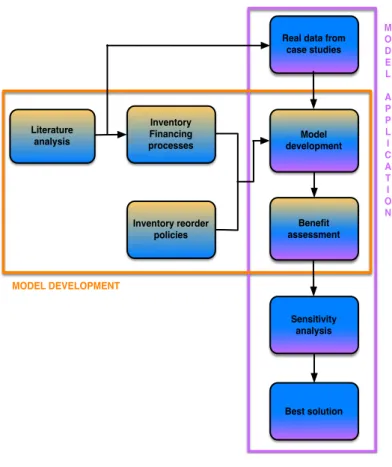
The methodology of this work is split in two main processes: one concerning the model development (orange frame in the Figure 0.1) and another concerning the model application (purple frame in the Figure 0.1).

The first one starts with the analysis of the literature that has already provided theoretical models of IF. Concerning the different inventory reorder policies, they have already been strongly accomplished and used in real work situations, so we direct implement them due to their high reliability. Then, once all the information and ideas are collected, we develop the model through two main passages: the model development and the benefits assessment. The former concerns the framework of the model, including all parameters definitions, formula computations

and processes advancement. The latter establishes the benefits achieved by each player and by the whole supply chain thereafter the implementation of an IIFS combined with a specific inventory reorder policy. The second process starts with the analysis of case studies, reports and academic documents in order to obtain real data needed for the practical application of the model. In this way, we are able to carry out a quantitative comparison between the different IF solutions. However, even if the application has been made using real data, the model is based on assumptions which make the results even an

Figure 0.1- Model methodology Literature analysis Inventory Financing processes Inventory reorder policies Model development Benefit assessment Real data from

case studies Sensitivity analysis Best solution MODEL DEVELOPMENT M O D E L A P P L I C A T I O N

(18)

approximation of the reality. Thus, in order to understand the robustness of the pursued results, we decided to deepen the research through a sensitivity analysis which allow us to figure out under which conditions each IF solution performs better results.

Model Description

We have created a quantitative benefits assessment model which allow the user to compute the profit of the whole supply chain thereafter the implementation of an IF solution under a specific inventory reorder policy. More in details, the model is based on analytical formulas, so it mathematically proves how different IF solutions, combined with specific inventory policies, can affect the profit of each involved actor and as consequence the profit of the entire supply chain. The model encloses the development of three different typologies of IF solutions, one represents a traditional solution (Traditional Mode) whereas the other two can be categorized as innovative ones, respectively Delegation Mode and Control Mode.

Concluding, in all the previous solutions of IF we always consider the retailer as the budget-constrained company of the supply chain, thus the model is based on its own perspective. Traditional Mode

The retailer’s purchase orders, being it a capital constrained firm, may be limited. Thus, it will try to borrow funds, through an IF solution. In this situation, the bank may grant a loan to the borrower (retailer) evaluating its credit risk based both on its initial capital and on the value of its inventory used as collateral. The 3PL carries out just traditional logistics services because its only one task is to transport the ordered good from the supplier to the retailer; thus, concerning the financing topic, the 3PL covers a complete passive role in this model. The main problem of this situation is that the bank has not possibility to screen the information about the retailer’s initial capital, so the latter can falsify it in order to obtain a lower interest, thus increasing its profit. Moreover, the bank is not able to carefully monitor the collateral due to the low level of visibility on retailer’s internal processes. High information asymmetry and low visibility between lender and borrower are the main limiting factor of the TM. Indeed, banks might refuse to grant loans under these conditions. This is also the main reason why, most of times, SMEs are not able to borrow loans from financial institutions.

We have easily modeled the TM always assuming the bank does not grant the loan to the SME (retailer), so we can consider the situation as a no-financing one.

(19)

Delegation Mode

This solution is designed to solve the kind of issue present in the TM; in particular, the Delegation Mode reduces significantly the high asymmetric information level and at the same time improves the visibility on the collateral between the financial provider and borrowing firm. In the DM, the 3PL assumes an important role because it helps the bank by sharing borrower’s real information and by tracking the collateral of the loan (e.g. inventory). After having assumed the retailer’s CCC turns negative thanks to the implementation of DM, we modeled this solution as in the Figure 0.2.

At the beginning, the retailer defines the amount of products to order with the purpose to satisfy the market demand [step 1.a]. The trigger point of the DM is when the retailer becomes aware that it has not enough funds to place the order, so it asks an Inventory Financing request to the bank. The retailer sends part of its inventory of Product_X (which represents the goods available to be pledged) to the 3PL’s warehouse [step 1.b]. After having received the goods, the 3PL starts to analyze and check the collateral conditions, then it shares all the information about the collateral with the bank [step 1.c]. Now, the bank is going to pay in advance the 3PL, on behalf of the retailer, the total cost of the services (e.g. collateral holding and monitoring) that it provides [step 1.d]. In the same period, the bank grants the loan to the retailer [step 1.e], which now has enough funds to place the order and specially to carry out the payment of W% of the order value to the supplier [step 1.f]. At t=r, the 3PL delivers the goods to the retailer [step 2.a] who starts to sell them to its customers [step 2.b] getting immediately the Y (%) of the sales value [step 2.c]. At t=j the retailer gets the remaining 1-Y% [step 3.a] of the total revenue and in t=h (in this case we suppose h=j) it pays the remaining part (1-W

(20)

%) of the order value placed at t=0 [step 3.b]. Concluding, in t=g the retailer has to payback the whole debt to the bank [step 4.a] and, just when this payment will be completed, the bank authorizes the 3PL to give the pledged goods back to the retailer [step 4.b].

With DM solution, it is possible solve the difficulty of the SME financing and decrease the bank’s risk at the same time. However, also in this solution, an important issue continues to persist: the retailer may divert funds in loans to a higher risk project, leaving the bank with a higher risk. As consequence, the latter would be unwilling to offer loans if it has not any chance to monitor the borrower’s real procurement behaviors.

Control Mode

In this solution of IF the 3PL provides not only logistics but also financing services. When the retailer has insufficient capital, the 3PL procures the products from the supplier through trade credit financing and then transports them to the retailer. The innovative feature of the CM is that financial provider (that now it is a logistic operator) offers trade credit and no longer a loan; in this way it also has total visibility on the retailer’s procurement behaviors, so the latter cannot divert funds in other high risk projects. Moreover, all the goods financed by trade credit must be moved just inside the logistics network of the 3PL. Acting as a conductor of all flows, the 3PL is able to solve all the problems present both in the previous solutions. Now the retailer has to

declare sincerely all the information requested and in addition it has no longer the possibility to divert the capital loans to other riskier project because the lending fund goes directly from the 3PL to the supplier. Also here we assume the retailer’s CCC turns negative after the implementation of CM and we modeled this situation as in the Figure 0.3.

At the beginning, as in the DM, the

retailer defines how many products ordering with the purpose to satisfy the market demand [step 1.a]; the trigger point of the CM is when the retailer becomes aware that it is

(21)

not able to place the order due to its lack in funds, so it asks an Inventory Financing request no longer to a bank but to a Logistic Operator which also offers financing services. Precondition to make the CM solution possible, is a multi-party agreement among all the players. After this, the next passage [step 1.b] is the retailer’s order placement whose value is partially paid (Q%) immediately by the financial provider via trade credit line [step 1.c]. After having received the first part of the payment, the supplier sends the goods that will be received by the retailer at t=r (it’s crucial to highlight that this shipping is moved and handled just by the 3PL-Bank in its own transportation network) [step 2.a]. Once the goods are received by the retailer, it starts selling them [step 2.b] to its customers who pay immediately the Y% of the total sale value [step 2.c]. At t=j, the retailer gains the remaining 1-Y% of the the total revenue [step 3.a] and in t=h (also in this case we suppose h=j) pays the supplier the remaining part (1-Q%) of the order value placed at t=0 [step 3.b]. To conclude, at t=g, the 3PL-Bank has to receive back the total value of the credit line increased by an interest rate [step 4.a].

Results

In order to test the reliability and accuracy, we performed an application by feeding the model with real data obtained from case studies, reports and academic documents. Furthermore, with the purpose of figuring out how the results change if the external scenario becomes different, we carried out a sensitivity analysis varying the values of three parameters: the standard deviation of the market demand, interest rate applied by the financial providers to the retailer and inventory level of Product_X available to be pledged (respectively 𝜎, i and 𝐼𝑛𝑣𝑒𝑛𝑡𝑜𝑟𝑦(𝑋)? @ABCDE). In particular, the sensitivity analysis has been

developed on three levels, where each of them represents a different combination of the previous parameters (see Figure 0.4).

Figure 0.4 - Sensitivity analysis process

The first level immediately reveals that the "profit gap" between innovative and traditional IF solutions increases if the variability of the demand grows. For “profit gap” we mean the

(22)

difference between the supply chain profits obtained by the application of an IIFS and a traditional one. In this way we are able to reply the first research question. Thanks to this level, we can also investigate and find a possible answer to the third research question. Specifically, varying the demand uncertainty level, we have studied how a specific inventory policy can affect the supply chain profit obtained after the application of an IIFS (DM or CM). Therefore, depending on which IIFS is adopted by the retailer, different results emerge (see Figure 0.5).

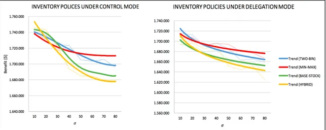
Figure 0.5 - Benefits trends of IIFSs according to different inventory policies

Under the Control Mode, when the demand standard deviation is low, Hybrid and Base-Stock systems perform better results because they allow the budget-constrained firm to reduce its management inventory costs, thus saving fund usable to issue the next order bigger. On the other hand, when the demand standard deviation takes on a medium-high level, the previous policies are not able anymore to face such demand, indeed the stock out costs overpass the potential savings of a periodic inventory control logic. Thus, Two-Bin and Min-Max systems, thanks to their continuous inventory control logic, become the best solutions which can ensure a greater profit for the whole supply chain. Specifically, the Min-Max system is better since it is still more flexible and dynamic than the Two-Bin one. Concerning the Delegation Mode situation, the best inventory policies result to be always the ones with a continuous inventory control logic (Two-Bin and Min-Max systems). The systems with a periodic inventory control logic, independently of the demand standard deviation level, generate always lower profits than Two-Bin and Min-Max policies. More in details, the Two-Bin system ensures better results when the level of demand standard deviation is low (𝜎 < 20), then the Min-Max system starts offering a higher supply chain profit. With the purpose to answer to the second research question, we change our analysis

(23)

perspective focusing on the comparison between the CM and DM, both always considered under the same inventory control logic. In order to express this comparison, we adopt the variable 𝜆JBK LAMNOP which is estimated as follows:

𝜆_JBK LAMNOP = 𝑆𝐶 𝑃𝑅𝑂𝐹𝐼𝑇_JBK LAMNOPYABCZAM [A\]− 𝑆𝐶 𝑃𝑅𝑂𝐹𝐼𝑇_JBK LAMNOP_]M]`aCNAB [A\]

In particular, in order to make the result as clear and direct as possible, we consider the difference between CM and DM, not for each inventory policy, but for each inventory control logic. Thus, we define the variables 𝜆YABCNBbAbE and 𝜆L]ZNA\NO as follows:

𝜆YABCNBbAbE =cdefghijc_n khiklm; 𝜆L]ZNA\NO=cglopqrfst_njcuvwxhy

Remaining in the first level of the analysis, we study how 𝜆YABCNBbAbE and 𝜆L]ZNA\NO behave, discovering that the difference between CM and DM under a continuous review logic increases when the variability of demand gets higher; instead under a periodic inventory control logic, 𝜆L]ZNA\NO follows the opposite trend, this because when the demand is highly variable the losses due to adopting a “wrong” logic to reorder the inventories (i.e. a periodic inventory control logic under a high demand uncertainty) are so high to almost nullify the benefits of a CM solution (see Figure 0.6).

Figure 0.6 - 𝝀𝑪𝒐𝒏𝒕𝒊𝒏𝒖𝒐𝒖𝒔 and 𝝀𝑷𝒆𝒓𝒊𝒐𝒅𝒊𝒄trends under different values of 𝝈

Moving to the second level of the analysis, we find out a relation between

𝑖𝑛𝑣𝑒𝑛𝑡𝑜𝑟𝑦(𝑋)? @ABCDE and the variables 𝜆YABCNBbAbE and 𝜆L]ZNA\NO (see Figure 0.7).

Specifically, when the first one assumes a low value, the difference between CM and DM gets very high in both the inventory control logics. This behavior makes sense because the DM, when the retailer has a very few amount of Product_X available to be pledged,

𝝀

[$

(24)

becomes very similar to the Traditional Mode (where the retailer can not pledge anything due to none IF solution is underway), hence the difference with a Control Mode is huge. Increasing the value of 𝑖𝑛𝑣𝑒𝑛𝑡𝑜𝑟𝑦(𝑋)? @ABCDE the difference between CM and DM decreases significantly, making the benefits of the two solutions very similar. Moreover, if we continue increasing the amount of Product_X, both the value of 𝜆YABCNBbAbE and 𝜆L]ZNA\NO slowly start to increase. We justify the last statement because now the Product_X can not be considered anymore as secondary product (this because we assumed the Product_X quantity proportional to its future demand).

Concluding, the third level of the analysis reveals that increasing the interest rate, also the difference between CM and DM proportionally increases in both the inventory control logics (see Figure 0.8). This because, in the DM, the bank applies the interest rate on the loan value plus other costs (e.g. collateral management cost), whereas in the CM, the 3PL-Bank applies the interest rate just on the value of the trade credit granted to the retailer. Thus, receiving the same amount of funding, in the CM the retailer pays a lower interest.

Figure 0.8 - 𝝀𝑪𝒐𝒏𝒕𝒊𝒏𝒖𝒐𝒖𝒔 and 𝝀𝑷𝒆𝒓𝒊𝒐𝒅𝒊𝒄 trends under different values of i

Figure 0.7 - 𝝀𝑪𝒐𝒏𝒕𝒊𝒏𝒖𝒐𝒖𝒔 and 𝝀𝑷𝒆𝒓𝒊𝒐𝒅𝒊𝒄trends under different values of 𝑰𝒏𝒗𝒆𝒏𝒕𝒐𝒓𝒚(𝑿)𝟑 𝒎𝒐𝒏𝒕𝒉𝒔

𝝀 [$ ] 𝝀 [$ ]

(25)

SOMMARIO

Introduzione

L’attuale situazione economica sta rendendo sempre più necessario lo sviluppo di nuove soluzioni di finanziamento che possano aiutare gli attori più deboli delle supply chain; infatti, regole severe, combinate con una forte sfiducia generale, impediscono ancora oggi alle PMI di ricevere finanziamenti adeguati. Quindi, quest’ultime non sono solo le aziende più deboli, ma anche le più rischiose, in quanto devono costantemente fronteggiare un elevato rischio di fallimento. In questo contesto, sono state sviluppate diverse soluzioni di Supply Chain Finance, tra le quali è presente l’Inventory Financing (IF). Quest’ultima è un tipo di prestito asset-based, cioè un prestito a breve termine concesso ad una società le cui scorte servono come garanzia per il provider finanziario; quindi, se l'azienda non potrà rimborsare il prestito, il provider finanziario diventerà il proprietario delle scorte.

Lo scopo di questa tesi è quello di valutare i benefici delle Soluzioni Innovative di Inventory Financing (IIFS). Più in dettaglio, confrontiamo i vantaggi di due IIFS, che chiameremo rispettivamente Delegation Mode (DM) e Control Mode (CM), ispirandoci alla terminologia adottata da Chen e Cai (2011). In particolare, il benchmark di riferimento, usato per la valutazione dei benefici del DM e del CM, è rappresentato da una soluzione tradizionale di IF che chiameremo Traditional Mode (TM).

Inoltre, valutiamo i vantaggi di una combinazione tra una specifica politica di riordino delle scorte (adottata dallo stesso attore che sta attuando la IIFS) e una IIFS. In particolare, prenderemo in considerazione due politiche di riordino riguardanti una logica continua di controllo del magazzino ("Two-Bin" e "Min-Max") e due per quanto riguarda una logica periodica di controllo del magazzino ("Base-Stock" e "Hybrid").

Infine, basiamo il nostro modello su una supply chain costituita da un fornitore, un operatore logistico (3PL), un provider finanziario ed un retailer; in particolare, quest’ultimo è l’attore critico in quanto dispone di una liquidità limitata (budget-constrained retailer).

Obiettivi

Gli obiettivi della nostra tesi possono essere sintetizzati sotto forma di tre Domande di Ricerca (DR).

(26)

DR1. Quanto una supply chain può beneficiare dall’implementazione, da parte dell’azienda budget-constrained, di una IIFS combinata con una specifica politica di riordino delle scorte?

Grazie al nostro modello di valutazione quantitativa dei benefici, possiamo confrontare le IIFS con una soluzione tradizionale di IF, guardando il profitto globale della supply chain generato dopo che l’azienda budget-constrained implementa contemporaneamente una specifica IIFS e una specifica politica di riordino delle scorte. Inoltre, grazie all’analisi di sensitività, siamo in grado di capire come i differenti profitti della supply chain cambiano all’aumentare della variabilità della domanda.

RQ 2. Quando il Delegation Mode genera benefici simili o addirittura migliori rispetto al Control Mode?

In accordo con Chen e Hu (2011), il Delegation model è una soluzione innovativa, ma non così innovativa come il Control model; pertanto essi presentano quest’ultima come una migliore e più profittevole soluzione di IF rispetto alla soluzione Delegation model. In questa tesi studiamo e analizziamo attentamente entrambe le soluzioni sopra menzionate attraverso lo sviluppo di, rispettivamente, il Delegation Mode e del Control Mode. Implementando il modello siamo in grado di investigare ed individuare se esiste un potenziale contesto dove il DM eguaglia, o addirittura supera, i benefici del CM. In altre parole, forniamo alla letteratura corrente uno strumento quantitativo che permetta all'utente di capire quale sia la migliore IIFS, date le specifiche condizioni iniziali e la politica di riordino delle scorte adottata dall’azienda budget-constrained.

RQ 3. Una specifica politica di riordino delle scorte, se combinata con una IIFS, influenza il profitto dell’intera supply chain?

Rispondiamo a questa domanda analizzando i benefici ottenuti dopo l'adozione di quattro diverse politiche di riordino delle scorte da parte dell’azienda budget-constrained. Quindi, calcoliamo il profitto della supply chain ottenuto in seguito all’implementazione di una specifica combinazione tra una IIFS e una delle quattro politiche di riordino delle scorte adottate. Quindi, per mezzo dell’analisi di sensitività, studiamo come i precedenti risultati cambiano al variare dell’incertezza della domanda.

Analisi della letteratura

Dal momento che la tematica dell’IF è abbastanza recente, abbiamo indagato diverse tipologie di fonti. La base più significativa dell’analisi della letteratura consiste in

(27)

pubblicazioni accademiche e articoli scientifici (57% del totale). Inoltre abbiamo considerato reports di conferenze specialistiche (15% del totale) e manuali (13% del totale). Questi riferimenti ci hanno fornito i processi operativi e alcune valutazioni qualitative e quantitative già presenti in letteratura. La restante parte è costituita da altre fonti (15% del totale) che sono principalmente tesi di laurea e casi di studio provenienti da siti web. Per concludere, i consigli del Prof. Xianfeng Chen (Fudan University) hanno ricoperto un ruolo importante nel nostro lavoro. In particolare, egli ci ha supportato lungo tutte le ricerche e lo sviluppo del modello, soprattutto per quanto riguarda la definizione delle assunzioni e delle formule su cui esso è basato.

Metodologia

La metodologia di questo lavoro è suddivisa in due processi principali: uno relativo allo sviluppo del modello (riquadro arancio della Figura 0.1) e un altro che riguarda l'applicazione del modello (riquadro viola della Figura 0.1).

Il primo processo parte con l'analisi della letteratura che fornisce i modelli teorici di IF. Per quanto riguarda le diverse politiche di riordino delle scorte, esse risultano già fortemente affermate e usate nella realtà lavorativa, pertanto sono state direttamente

implementate nel modello grazie alla loro elevata credibilità. In seguito, si arriva al cuore del processo che è rappresentato da due passaggi principali: lo sviluppo del modello e la valutazione dei benefici. Il primo passaggio riguarda la struttura del modello, cioè tutte le definizioni dei parametri, delle formule e dei processi di avanzamento. Il secondo passaggio determina i benefici ottenuti da ogni attore e da tutta la supply chain in seguito all'attuazione di una IIFS combinata con una specifica politica di riordino delle scorte.

Figura 0.4 - Metodologia del modello Literature analysis Inventory Financing processes Inventory reorder policies Model development Benefit assessment Real data from

case studies Sensitivity analysis Best solution MODEL DEVELOPMENT M O D E L A P P L I C A T I O N

(28)

Il secondo processo parte con l’analisi di casi di studio, reports e documenti accademici, con lo scopo di ottenere dati reali necessari per l’applicazione pratica del modello. In questo modo, siamo in grado di effettuare una comparazione quantitativa tra differenti soluzioni di IF. Tuttavia, anche se l’applicazione viene eseguita con dati reali, il modello è basato su assunzioni, le quali rendono i risultati ancora un’approssimazione della realtà. Quindi, con l’obiettivo di capire la robustezza dei risultati perseguiti, abbiamo deciso di approfondire la ricerca effettuando un’analisi di sensitività che ci permetta di valutare sotto quali condizioni ogni soluzione di IF ottiene i migliori risultati.

Descrizione del Modello

Abbiamo creato un modello quantitativo di stima dei benefici che permetta all’utente di valutare il profitto di ogni singolo attore e dell’intera supply chain in seguito all’implementazione simultanea di una soluzione di IF e di una specifica politica di riordino delle scorte. In particolare, essendo basato su formule analitiche, il modello effettua una valutazione matematica di come differenti soluzioni di IF, combinate con determinate politiche di gestione del magazzino, agiscono sul profitto di ogni singolo attore della supply chain e di conseguenza anche sul profitto della supply chain stessa. Il modello racchiude al suo interno lo sviluppo di tre differenti soluzioni di IF: una rappresenta una soluzione tradizionale (Traditional Mode), invece le restanti due descrivono soluzioni innovative di IF, rispettivamente il Delegation Mode e il Control Mode.

Infine, in tutte e tre le diverse situazioni, il retailer viene considerato come l’attore critico che implementa la soluzione di IF, pertanto il modello è strutturato sul suo punto di vista. Traditional Mode

Gli ordini di acquisto del retailer, a causa dei suoi problemi di liquidità, potrebbero subire forti limitazioni. Per evitare che questo accada, esso cercherà di ottenere finanziamenti tramite l’implementazione di una soluzione di IF. In una tale situazione, la banca prima di concedere il prestito valuta il livello di rischiosità del retailer analizzando sia il suo capitale iniziale sia il valore della merce impegnata come collaterale. L’operatore logistico svolge solo la funzione di trasporto della merce; pertanto esso ha un ruolo completamente passivo per quanto riguarda i finanziamenti che avvengono nella supply chain.

(29)

Il problema principale di questa situazione è che la banca non ha alcuna visibilità sulle informazioni inerenti al capitale del retailer, pertanto quest’ultimo potrebbe modificare le sue informazioni ottenendo un tasso di interesse inferiore ed aumentando così i suoi profitti. Inoltre la banca non è in grado di mantenere costantemente monitorato il collaterale a causa della poca visibilità concessa dal retailer sui suoi processi interni. Alta asimmetria informativa e bassa visibilità tra la parte che concede il prestito e quella che lo riceve sono il limite principale del TM. Infatti le banche potrebbero rifiutarsi di concedere prestiti in queste circostanze. Questo fattore è spesso la principale causa per cui le PMI non sono in grado di accedere a prestiti offerti da istituti finanziari.

Abbiamo semplificato la modellizzazione del TM assumendo sempre che la banca non conceda alcun prestito alla PMI (retailer), pertanto è come se fosse una una situazione in cui non è presente alcun tipo di finanziamento.

Delegation Mode

Questa soluzione è stata sviluppata con lo scopo di sanare le problematiche presenti in una situazione tradizionale di IF. In particolare, il DM riduce significativamente l’alta asimmetria informativa e, allo stesso tempo, migliora la visibilità sul collaterale tra la parte concedente il prestito e quella

destinata a riceverlo. Nel DM l’operatore logistico comincia a ricoprire un ruolo importante all’interno della supply chain in quanto condivide con la banca informazioni attendibili sul retailer ed inoltre svolge l’attività di monitoraggio del collaterale. Dopo aver assunto che il CCC del retailer diventi negativo grazie all’implementazione del DM, abbiamo modellizzato tale soluzione come riportato nella Figura 0.2.

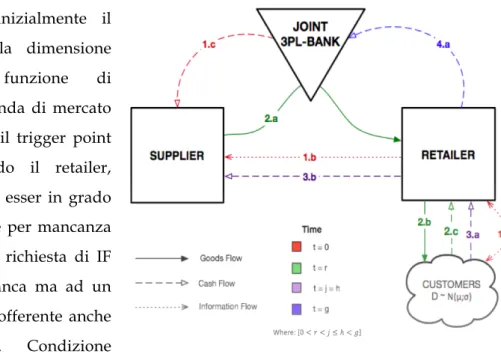
Il primo passaggio prevede che il retailer vada a definire la dimensione dell’ordine con l’obiettivo di riuscire a soddisfare la domanda del mercato prevista [step 1.a]. Il trigger

(30)

point del DM avviene quando il retailer viene a conoscenza di non essere in grado di emettere l’ordine poichè non dispone di fondi sufficienti, quindi invia una richiesta di IF alla banca. In seguito il retailer invia parte delle sue scorte di Product_X (rappresentante i prodotti disponibili ad esser impegnati) al magazzino del 3PL [step 1.b]. Dopo aver ricevuto il collaterale, il 3PL inizia ad analizzarlo e a controllare le sue condizioni per poi procedere con l’invio e la condivisione di tutte queste informazioni con la banca [step 1.c]. La banca paga al 3PL, per conto del retailer, il costo dei servizi che esso sosterrà (per esempio la gestione e il monitoraggio del collaterale) [step 1.d]. Nello stesso periodo la banca concede il prestito al retailer [step 1.e], il quale ora dispone di fondi sufficienti per emanare l’ordine di acquisto ed in particolare per pagare subito al fornitore un importo pari al W % del valore dell’ordine [step 1.f]. In t=r il 3PL consegna la merce al retailer [step 2.a], il quale inizia subito l’attività di vendita [step 2.b] incassando immediatamente una somma pari al Y % del valore totale delle vendite [step 2.c]. In t=j il retailer incassa la restante parte delle vendite pari a 1-Y% [step 3.a] e in t=h (in questa situazione abbiamo assunto h=j) esso paga al fornitore la restante parte (1-W%) dell’ordine effettuato in t=0 [step 3.b]. Infine in t=g il retailer ripaga il prestito alla banca [step 4.a] e, solo dopo aver completato tale pagamento, la banca informa il 3PL di restituire il collaterale al retailer [step 4.b].

Con una soluzione di DM, è possibile risolvere le difficoltà finanziarie in cui intercorrono le PMI e allo stesso tempo ridurre il rischio che le banche corrono quando concedono un finanziamento. Tuttavia in questa soluzione persiste un’altra problematica: il retailer potrebbe divergere i fondi ottenuti tramite il prestito in progetti molto rischiosi facendo così aumentare i rischi per la banca. Di conseguenza quest’ultima potrebbe decidere di non concedere il prestito senza prima aver avuto completa visibilità sui processi di acquisto del retailer.

Control Mode

In questa soluzione di IF il 3PL offre non solo servizi logistici, ma anche servizi finanziari. Quando il retailer ha fondi insufficienti per effettuare un ordine, il 3PL gli finanzia buona parte di esso tramite una linea di credito. In seguito lo stesso operatore logistico si incarica del trasporto e della consegna della merce. La caratteristica innovativa del CM è che il provider di servizi finanziari (che in questa soluzione risulta esser anche l’operatore logistico) offre un credito e non più un prestito; in questo modo esso ha piena visibilità anche sugli acquisti del retailer, il quale non ha più alcuna possibilità di divergere i finanziamenti in progetti ad alto rischio. Inoltre tutta la merce finanziata tramite il credito

(31)

offerto dal 3PL viene movimentato dallo stesso, esclusivamente all’interno della sua rete logistica. Agendo come gestore di tutti flussi della supply chain, il 3PL è quindi in grado di risolvere i problemi sorti nelle precedenti soluzioni. Ora il retailer è costretto a dichiarare correttamente tutte le informazioni richieste ed inoltre non ha più nessuna chance di divergere il prestito in progetti ad alto rischio, questo poiché, trattandosi di un credito, il finanziamento arriva direttamente al fornitore.

Anche qui, dopo aver assunto che il CCC del retailer diventi negativo in seguito all’implementazione del CM, abbiamo modellizzato tale soluzione come mostrato in Figura 0.3.

Come nel DM, inizialmente il retailer definisce la dimensione dell’ordine in funzione di soddisfare la domanda di mercato prevista [step 1.a]; il trigger point del CM è quando il retailer, consapevole di non esser in grado di emettere l’ordine per mancanza di fondi, invia una richiesta di IF non più ad una banca ma ad un operatore logistico offerente anche servizi finanziari. Condizione necessaria affinché si possa

realizzare il CM è la presenza di un accordo multilaterale tra tutti gli attori della supply chain. Dopo aver definito il contratto, il retailer effettua l’ordine [step 1.b] di cui una parte (Q%) viene immediatamente pagata dal 3PL attraverso la linea di credito offerta [step 1.c]. Una volta ricevuta la prima parte del pagamento, il fornitore spedisce la merce al retailer, il quale la riceverà in t=r (è fondamentale sottolineare che questa spedizione è movimentata e gestita esclusivamente dalla rete di trasporto del 3PL) [step 2.a]. Una volta ricevuta la merce, il retailer inizia subito la vendita [step 2.b], incassando immediatamente una somma pari al Y % del valore totale delle vendite [step 2.c]. In t=j il retailer incassa la restante parte delle vendite pari a 1-Y% [step 3.a] e in t=h (anche in questa situazione supponiamo essere h=j) esso paga al fornitore la rimanente parte (1-Q%) dell’ordine effettuato in t=0 [step 3.b]. Infine in t=g il retailer restituisce al 3PL una somma pari all’ammontare del credito concesso incrementato di un tasso di interesse [step 4.a].

(32)

Risultati

Con lo scopo di testarne l’affidabilità e l’accuratezza, abbiamo eseguito un’applicazione del modello alimentandolo con dei dati reali provenienti da casi di studio, reports e documenti accademici. In aggiunta, per capire come i risultati cambiano al variare del contesto esterno, abbiamo effettuato un’analisi di sensitività basata su tre parametri: la deviazione standard della domanda, il tasso d’interesse applicato dal financial provider al retailer e la quantità di scorta del Product_X disponibile per essere impegnata (rispettivamente 𝜎, i e 𝐼𝑛𝑣𝑒𝑛𝑡𝑜𝑟𝑦(𝑋)? @ABCDE). In particolare, l’analisi è stata sviluppata su tre livelli, dove ognuno di essi rappresenta una differente combinazione dei precedenti parametri (vedi Figura 0.4).

Figura 0.4 - Processo dell’analisi di sensitività

Il primo livello rivela immediatamente che il “profit gap” tra una IIFS e una soluzione tradizionale di IF aumenta all’aumentare della variabilità della domanda. Dove il “profit gap” è la differenza tra i profitti della supply chain ottenuti rispettivamente dall’applicazione di una IIFS e da una soluzione tradizionale di IF. In questo modo rispondiamo alla prima domanda di ricerca.

Grazie a questo livello, siamo anche in grado di investigare e trovare una possibile risposta alla terza domanda di ricerca. In particolare, variando il livello d’incertezza della domanda, abbiamo studiato come una specifica politica di riordino delle scorte influenza il profitto della supply chain ottenuto dopo che il retailer ha implementato una IIFS (DM o CM).

(33)

Sulla base della IIFS implementata, emergono differenti risultati (vedi Figura 0.5).

Nella situazione di CM, quando la deviazione standard della domanda è bassa, le politiche Hybrid e Base-Stock sono le migliori perché permettono all’azienda “budget constrained” di ridurre i suoi costi di gestione delle scorte, risparmiando così liquidità per eseguire un ordine futuro più grande. Al contrario, quando la deviazione standard della domanda assume un valore medio-alto, le precedenti politiche non sono più in grado di far fronte a tale domanda, infatti i costi di stock-out superano i potenziali risparmi di una logica periodica di controllo del magazzino. Quindi le politiche Two-Bin e Min-Max, grazie alla loro logica continua di controllo del magazzino, diventano le migliori soluzioni per quanto riguarda il profitto dell’intera supply chain. Più in dettaglio la politica Min-Max è migliore, poiché ancora più flessibile e dinamica rispetto a quella Two-Bin.

Per quanto riguarda la situazione di DM, le migliori politiche di riordino delle scorte risultano essere sempre quelle con una logica continua di controllo del magazzino (Two-Bin e Min-Max). Al contrario, le politiche con una logica periodica di controllo, indipendentemente dall’incertezza della domanda, generano sempre benefici minori. Più in dettaglio, la politica Two-Bin assicura i migliori risultati se la deviazione standard della domanda è bassa (𝜎 < 20); quando invece l’incertezza della domanda inizia ad aumentare la politica Min-Max diventa quella predominante.

Con l’obiettivo di rispondere alla seconda domanda di ricerca, cambiamo la prospettiva dell’analisi focalizzandoci sulla comparazione tra CM e DM, considerandoli sempre sotto la medesima logica di controllo del magazzino. Quindi, per esprimere questa comparazione, adottiamo la variabile 𝜆JBK LAMNOP , che è stimata come segue:

𝜆_JBK LAMNOP = 𝑆𝐶 𝑃𝑅𝑂𝐹𝐼𝑇_JBK LAMNOPYABCZAM [A\]_{− 𝑆𝐶 𝑃𝑅𝑂𝐹𝐼𝑇}

JBK LAMNOP_]M]`aCNAB [A\]

In particolare, al fine di rendere i risultati più chiari e diretti, andiamo a considerare la differenza tra CM e DM, non per ogni singola politica di riordino, ma più semplicemente per ogni logica di controllo del magazzino. Definiamo quindi le variabili 𝜆YABCNBbAbE e 𝜆_L]ZNA\NO come segue:

𝜆YABCNBbAbE =cdefghijc_n khiklm; 𝜆L]ZNA\NO=cglopqrfst_njcuvwxhy

Restando nel primo livello dell’analisi, studiamo come la variabile 𝜆YABCNBbAbE e 𝜆L]ZNA\NO si comportano, scoprendo che la differenza tra CM e DM sotto una logica di controllo continuo del magazzino aumenta all’aumentare della variabilità della domanda; al

(34)

contrario, sotto una logica di controllo periodico del magazzino, la variabile 𝜆L]ZNA\NO segue il trend opposto, questo perché quando la domanda è molto variabile le perdite causate dall’adozione di una logica “errata” di controllo delle scorte (cioè una logica di controllo periodico di magazzino sotto un elevato livello di incertezza della domanda) sono così elevate da quasi annullare i benefici di una soluzione di CM (vedi figura 0.6).

Figura 0.6 - 𝝀𝑪𝒐𝒏𝒕𝒊𝒏𝒐𝒖𝒔 e 𝝀𝑷𝒆𝒓𝒊𝒐𝒅𝒊𝒄 trends secondo differenti valori di 𝝈

Spostandoci nel secondo livello dell’analisi, scopriamo una relazione tra la variabile 𝑖𝑛𝑣𝑒𝑛𝑡𝑜𝑟𝑦(𝑋)? @ABCDE e le variabili 𝜆YABCNBAbE e 𝜆L]ZNA\NO (vedi Figura 0.7). Nello specifico, quando la prima risulta bassa, la differenza tra CM e DM è molto elevata per entrambe le logiche di controllo. Questo comportamento ha senso poiché il DM, quando il retailer possiede una bassa quantità del Product_X disponibile per essere impegnata, diventa molto simile al TM (dove il retailer non impegna nulla in quanto non attiva alcuna soluzione di IF), quindi la differenza con il CM è molto elevata.

Aumentando l’ammontare di 𝑖𝑛𝑣𝑒𝑛𝑡𝑜𝑟𝑦(𝑋)? @ABCDE la differenza tra CM e DM diminuisce

significatamente, rendendo i benefici delle due soluzioni molto simili. Tuttavia se continuiamo ad aumentare l’ammontare del Product_X, il valore di entrambe le variabili 𝜆YABCNBAbE e 𝜆L]ZNA\NO inizia lentamente a risalire. Legittimiamo quest’ultimo risultato in quanto ora il Product_X non può essere più considerato come un prodotto secondario (poiché è stato assunto che la quantità di Product_X è direttamente proporzionale alla sua domanda futura).

(35)

Infine, il terzo livello dell’analisi rivela che la differenza tra CM e DM aumenta in modo proporzionale al valore del tasso d’interesse ed indipendentemente dalla logica di controllo del magazzino adottata dal retailer (vedi Figura 0.8). Questo perché, nel DM, la banca applica un tasso d’interesse su un imponibile costituito dal valore del prestito e da altri costi sostenuti (per es. i costi di gestione del collaterale), mentre nel CM, il 3PL-Bank applica il tasso d’interesse solo sul valore del credito concesso al retailer. Quindi, a parità di valore del presito ricevuto, nel CM il retailer paga un interesse totale minore.

Figura 0.7 - 𝝀𝑪𝒐𝒏𝒕𝒊𝒏𝒐𝒖𝒔 e 𝝀𝑷𝒆𝒓𝒊𝒐𝒅𝒊𝒄 trends secondo differenti valori di 𝐈𝐧𝐯𝐞𝐧𝐭𝐨𝐫𝐲(𝐗)𝟑 𝐦𝐨𝐧𝐭𝐡𝐬

(36)

(37)

LITERATURE REVIEW

This chapter illustrates the most relevant contributions in the literature that represent a fundamental theoretical basis for the development of this work. We first introduce the reader to the concepts of supply chain, supply chain management and supply chain finance. Then we focus on the Inventory Financing (IF) solution, which is the core of this thesis, stating its definitions, frameworks and describing its processes and benefits.

“Business practices of the future will be defined in a new unit of analysis: the supply chain (not the individual organization) […] will become the effective unit of competition.”

(Handfield, 2002) The supply chain concept has been subjected to huge evolution in the last 40 years, since this topic has been intensely studied.

A supply chain is a system of organizations, people, activities, information and resources involved in moving a product or service from supplier to customer. Supply chain activities involve the transformation of natural resources, raw materials, and components into a finished product that is delivered to the end customer (Van Drunen, KPMG1_{, 2011).}

Poirier and Quinn (2004) offered a five-phase supply chain maturity model in their article “How are we doing? A Survey of Supply Chain Progress” (see Figure 1.1). The first phase of the Poirier and Quinn model involves enterprise integration that strives for corporate alignment (vertical integration), whereas the second phase has the aim to achieve corporate excellence. The focus of these first two phases is internal (i.e. intra-enterprise).

In the third phase, organizations look externally to develop partner collaboration. In phase four, supply chain stakeholders work to create value chain collaboration (improved supply chain transparency and visibility). The aim of these last two phases was to reduce costs while increasing products quality because each partner is now focused on just one part of the process.

1_{KPMG was founded in 1987 after merging Peat Marwick International and Klynveld Main Goerdeler. It is a}

global network of professional firms providing Audit, Tax and Advisory services. They operate in 155 countries and have more than 162,000 people working in member firms around the world. Its global headquarter is located in Amsterdam, Netherlands.

(38)

In the fifth and final phase, when business is becoming too complex for just a single company, supply chain stakeholders achieve full network connectivity in order to better respond to a more dynamic demand and to accelerate the globalization pace. Thus, enterprises started to forge closer alliances with their trading partners, trying to retain customers and maintain the leading edge in an increasingly competitive market.

To conclude, as Done (2011) said, companies along the whole supply chains must become more integrated by increasing the collaboration between upstream and downstream partners. This would allow them to achieve better results and benefits. Nowadays, however, the majority of existing supply chains are still focused on asset, data and information elements of exchange between supply chain partners, but an optimal integration and collaboration clearly require the exchange of more complex elements at the expertise and knowledge levels.

(39)

Supply Chain Definitions

When an organization tries to focus on supply chain management, its leaders must determine what the supply chain encompasses. Just as you can not manage what you do not measure, you can not plan and execute what you have not clearly defined. Hence, it is important to articulate the overall purpose, scope, and components of a supply chain (Gibson et al. 2013).

Below there are useful supply chain definitions that highlight critical aspects of a supply chain:

• From Christopher (1992) — The network of organizations that are involved, through upstream and downstream linkages, in the different processes and activities that produce value in the form of products and services delivered to the ultimate consumer;

• From the CSCMP2_{(2010) — The material and informational interchanges in the}

logistical process, stretching from acquisition of raw materials to delivery of finished products to the end user. All vendors, service providers, and customers are links in the supply chain;

• From Mentzer et al. (2001) — Supply chain is defined as a set of three or more entities (i.e. organizations or individuals) directly involved in the upstream and downstream flows of products, services, finances, and/or information from a source to a customer; • From Coyle et al. (2013) — A series of integrated enterprises that must share information and coordinate physical execution to ensure a smooth, integrated flow of goods, services, information, and cash through the pipeline.

One important feature of these definitions is the concept of an integrated network or system.

A simplistic description of a supply chain, as represented in Figure 1.2, suggests that a supply chain is linear, with organizations linked to their upstream suppliers and downstream customers.

2_{CSCMP (Council of Supply Chain Management Professionals): Founded in 1963, the Council of Supply} Chain Management Professionals (CSCMP) is the preeminent worldwide professional association dedicated to the advancement and dissemination of research and knowledge on supply chain management. With over 8,500 members representing nearly all industry sectors, government and academia from 67 countries, CSCMP members are the leading practitioners and authorities in the fields of logistics and supply chain management.

(40)

Specifically, the supply chain encompasses the steps to get a product or a service from the supplier to the customer.

Supply chains include every company that comes into contact with a particular product (H. Chen et al., 2014); for example, the supply chain for most products will encompass all the companies manufacturing parts for the product, assembling it, delivering it and selling it.

Structure and Actors

Supply chains require a multiplicity of relationships and numerous paths through which products and information travel (Lambert and Cooper, 2000). This is better reflected by the Figure 1.3, in which the supply chain is a network of participants and resources. To gain maximum benefit from the supply chain, a company must dynamically draw upon its available internal capabilities and the external resources of its supply chain network to fulfill customer requirements.

This network of organizations, with their facilities and transportation linkages, facilitate the procurement, the transformation of materials into desired products and distribution to customers.

Moreover, as Londe and Masters (1994) said, a supply chain needs to be a set of actors that pass materials forward. In fact, normally, several independent players are involved in manufacturing a product and in placing it in the hands of the end user in a supply chain. These members may be raw material and component producers, product assemblers, wholesalers, retailer merchants and transportation companies.