by
Giovanni Morleo, Marianna Gilli, Massimiliano Mazzanti
Environmental Performances in Europe: An Empirical Analysis of
the Convergence among Manufacturing Sectors
SEEDS is an interuniversity research centre. It develops research and higher education projects in the fields of ecological and environmental economics, with a special focus on the role of policy and innovation. Main fields of action are environmental policy, economics of innovation, energy economics and policy, economic evaluation by stated preference techniques, waste management and policy, climate change and development.
The SEEDS Working Paper Series are indexed in RePEc and Google Scholar. Papers can be downloaded free of charge from the following websites: http://www.sustainability-seeds.org/.
Enquiries:[email protected]
SEEDS Working Paper 05/2019 March 2019
By Giovanni Morleo, Marianna Gilli, Massimiliano Mazzanti
This is a pre-print document of an article that has been published at Revue d'économie industrielle, available at:https://www.cairn.info/revue-d-economie-industrielle-2017-3-page-21.htm?contenu=resume
1
Environmental Performances in Europe: An Empirical Analysis of the
Convergence among Manufacturing Sectors
Giovanni Morleo*; Marianna Gilli**; Massimiliano Mazzanti***
Abstract
This study focuses on the environmental performances of the European manufacturing industry. Our aim is to test the existence of both absolute and conditional β-convergence as well as σ-convergence in the environmental productivity (i.e., for each sector, the ratio between value added and carbon dioxide emissions) of 14 sectors for the period 1995-2009 using data from the WIOD database. The results support the hypothesis of β-convergence and highlight other factors such as trade openness. In addition, the results indicate that the sectorial share of value added can affect sectorial environmental performances, as shown by a higher speed of convergence. No statistical evidence of σ-convergence is found.
Keywords: environmental performances; manufacturing industry; β-convergence; σ-convergence; sector performances
Subject classification codes: L52 Q53 Q55
* Department of Economics and Management, via Voltapaletto 11, 44121 – Ferrara (Italy), [email protected]
** Department of Economics and Management, via Voltapaletto 11, 44121 – Ferrara (Italy), [email protected]
*** Department of Economics and Management, Via Voltapaletto 11, 44121 – Ferrara (Italy) [email protected]
2
Environmental Performances in Europe: An Empirical Analysis of the
Convergence among Manufacturing Sectors
1 Introduction
In recent decades, political institutions and public opinion have shown a growing interest in issues related to the environment and climate change. From this perspective, in the scientific community, there is broad consensus regarding the need for limiting global warming below 2 °C with respect to preindustrial period temperatures to avoid damage that would lead to more frequent and serious environmental disasters. During the recent international agreement on environmental issues signed at the 21st Conference of Parties (COP21), 195 State parties committed to limiting their polluting emissions to ensure that the increase of global temperatures remains well below 2 °C (UNFCCC, 2015; Robbins, 2016).1
Given the political significance of environmental issues, both the hard and social sciences show interest in debates regarding pollution and its link with human activities, such as the production of goods and services. Several theoretical, methodological and empirical studies in the economics literature relate to the topic of the economic and environmental impacts of reducing CO2 (carbon dioxide) emissions.
In addition to the well-known theory of the Environmental Kuznets Curve (ECK) that outlines that the relation between economic growth and environmental degradation that shows an inverted-U shape (see Carson, 2010 and Kijima et al., 2010, for a review on this subject), there certain studies have attempted to provide evidence for this relation. In the recent work of Calcagnini, Giombini and Travaglini (2016), the authors test whether significant relationships exist between labour productivity and energy intensity and between labour productivity and per capita emissions.
Furthermore, they analyse the possible effects of demand and supply shocks on the short-term and long-term trends of these variables. Other studies have focused on researching the drivers of pollution at the firm level and examining the effects of factor intensities, size, efficiency, technological innovations, environmental regulations (see for example Cole, Elliott and Shimamoto, 2005), and the role of public policies such as the introduction of environmental Pigouvian taxes and emission trading schemes.
Among the most discussed issues, increasingly, scholars are analysing the convergence patterns among polluting emissions at country levels (see for example: Strazicich and List, 2003; Stegman and McKibbin, 2005; Aldy, 2006; Lee and Chang, 2008). This study also focuses on this topic.
1In the final version of the document, all the countries agreed to use the same system of measurement,
control emissions and meet every 5 years to assess progress in emission abatement and define new targets. Furthermore, advanced countries agreed to allocate resources to developing countries to facilitate their transition to green energies (up to 100 billion dollars by 2020). Despite these measures, certain scholars have criticized the agreement since it creates non-binding standards and gives countries the discretion to self-determine the amount of polluting emissions they seek to reduce (Robbins, 2016).
3
For economists, the term ‘convergence’ is related to the analysis of economic growth disparities across countries (Barro and Sala-i-Martin, 1991). In its original application, convergence was a means to study the economic growth process in developing countries. Specifically, convergence was used to assess if the rate of economic growth was higher in developing countries than in advanced economies, which would reduce income inequalities. The purpose of this study is to use the conceptual framework of convergence and apply it to countries’ environmental performance, in the attempt to assess if it is levelling off across the European Union (EU) countries. Indeed, we believe that environmental regulation can reduce emissions in the top polluting sectors, particularly those that are less efficient. Policies such as the EU Emission Trading Scheme (EU-ETS), which set a common cap and a common market for tradable permits, can lead to a convergence of the environmental performances of countries in the EU.
The issue of convergence as related to environmental performances is also relevant from a political point of view. As Aldy (2006) argues, the more plausible it is that a convergence process has begun and the environmental performances of the least advanced countries is moving towards those of developed countries, the more willing developing countries would be to commit to emission abatement goals during
negotiations.
We use data obtained from the WIOD database to study the environmental performances of 27 European countries (all the current members of the EU, except for Croatia) for the period 1995-2009 and apply the same methodology used by Rodrik (2013). We consider the European context because of the great policy efforts shown in climate change mitigation, particularly regarding CO2 emissions. Furthermore, the
members of the European Union (EU) are diversified in terms of both economic and environmental performances (i.e., the newest member states had not developed an environmental commitment as stringent as the EU prior to their participation in the Union; therefore, we expect their initial levels of CO2 emissions to be higher).
According to the European Environment Agency (2015), the European Union is the third polluter in the world after China and the USA. The EU28’s emissions were 4,477 million tonnes of CO2-equivalent in 2013.2 Germany, the United Kingdom, France, Italy
and Poland account for 63.5% of total emissions. As for the polluting agents, CO2 is the
top greenhouse gas in terms of amount emitted (3,650 million of tonnes), followed by methane (CH4), nitrogen monoxide (N2O) and hydrofluorocarbons (HFC), which are
other important GHGs.
In our analysis, environmental performances are measured using an indicator of environmental productivity computed as the ratio between value added and carbon dioxide emissions, which was first introduced by Repetto (1990). According to the author, although the cost of non-market outputs, such as CO2 emissions, is important,
researchers should account for their value in terms of the “environmental dimension of productivity change” (Repetto, 1990, p. 34). Marin (2012) empirically applied this
4
concept to study the effects of regulations, technological change, investments and energy prices on environmental efficiency improvements. To the best of our knowledge, this study is the first to use this indicator for a convergence analysis at the sectorial level. This study contributes to the existing literature because our dependent variable considers the relation between the economic and environmental performances of a sector, which is a crucial aspect that should be considered to ensure competitiveness in the EU manufacturing sector.
Analysing the convergence of this indicator can offer several meaningful insights regarding the EU policy-making processes. An improvement in this indicator could occur because of either a decrease in CO2 emissions while the VA remains
constant (i.e., an improvement in environmental performances strictly as intended) or an increase in VA while CO2 remains constant (i.e., an improvement in economic
performance). This is consistent with the achievement of both environmental policy objectives (e.g., the correct functioning of the EU-ETS) and industrial policy objectives.
As in Rodrik (2013), we focus on manufacturing sectors and do so for two primary reasons. First, manufacturing industries account for a large share of CO2
emissions. According to Eurostat, CO2 emissions related to manufacturing activities
amounted to 836.5 million tonnes in 2013, representing 28% of total emissions.3 Second, these same industries are the target of complex EU climate change mitigation strategies, such as the Emission Trading Scheme (ETS). Despite structural changes in the European economy that imply a growth in the value added produced by the service sector and a slowdown in the relative importance of the manufacturing sector,
addressing issues related to polluting emissions is pivotal for reaching EU climate policy goals. As the European Environmental Agency explains, manufacturing
industries show better performances from a dynamic point of view and can adapt to eco-innovations and efficiency improvements; therefore, they are more capable of reducing their emissions over time (EEA, 2014). Thus, a reduction in the industrial emissions will contribute significantly and positively to the environmental impact of the aggregate economy. Moreover, the manufacturing sector continues to be crucial for the economic development in Europe, as witnessed by the European Commission (2014), which claims that an “industrial renaissance” is necessary for the continent and has defined targets such as industrial activities generating 20% of the EU GDP by 2020.
The remainder of this paper is organized as follows: Section 2 presents a synthetic review of the literature regarding the convergence in environmental
economics; Section 3 addresses the methodology, while Section 4 explains the sources of data. The results are discussed in Section 5 and Section 6 concludes.
3 The most polluting economic activity in the EU27 is the production and supply of energy and gas (1191
million tonnes, 39.5% of the total); other relevant sectors are transport (485 million tonnes, 16%) and agriculture (100.5 million tonnes, 3.3%).
5
2 Literature review
The vast majority of studies regarding the convergence of environmental performances focuses on variables such as polluting emissions. The trend of polluting emissions and the existence of convergence patterns became a major issue in the economic literature in the 90’s. As Islam (2003) argues in his study of income convergence, scholars have employed different methodologies that have resulted in conflicting empirical results. For this analysis, three of these methodologies are relevant, i.e., β-convergence, σ-convergence and stochastic convergence.4
Β-convergence occurs when countries with lower levels of per capita (or relative) emissions experience higher growth rates of emissions. The β-convergence focuses on the relationship between the initial level of per capita polluting emissions and its growth rate. Using this definition, convergence occurs when higher growth rates of a variable, on average, correspond to low initial levels (negative relation). In the context of polluting emissions, this implies that low-polluting countries show increasing per capita pollution over time. Among the scholars who have applied this definition, Strazicich and List (2003) find convergence among per capita CO2 emissions of 21
industrialized countries during the period from 1960 to the end of the 1990s. Moreover, their results emphasize the role of fuel prices and average temperatures in determining the timing of the convergence process.
Stegman and McKibbin (2005) find weak evidence for absolute β-convergence, using data for 91 non-OECD countries during the period 1950-2000. Finally, Lee and Chang (2008) use data for OECD countries from 1960 to 2000 and determine that only 7 countries are converging in terms of emissions according.
Another concept of convergence is σ-convergence. This definition considers the variability of distribution, i.e., the trend of an appropriate measure of the statistical dispersion of a variable (e.g., standard deviation) over time. To clarify, σ-convergence exists when the trend of the statistical dispersion decreases over time, which indicates a gradual convergence towards the mean of the distribution (Islam, 2003). For example, Aldy (2006) and Panopoulou and Pantelidis (2009) use data on per capita emissions to study σ-convergence. Both studies examine trends in the variability measures for the distribution of per capita emissions. Aldy (2006) provides evidence to support the convergence hypothesis for a sub-sample of OECD countries; the entire sample included 88 countries. Panopoulou and Pantelidis (2009) use data for 128 countries from 1960 to 2003 and test for the convergence of emissions for both the overall sample and, in alignment with Phillips and Sul (2007), for a selected group of countries (“club convergence”5). Although there is no evidence of σ-convergence in the overall sample,
4Islam (2003) offers a complete overview of the different definitions and analytical techniques used in
the convergence literature.
5 The term, club convergence, indicates a search for convergence in groups of countries that
have similar levels of certain measurable factors (e.g., income, education, or polluting emissions). In this case, countries with similar characteristics (e.g., advanced economies or
6
they highlight its existence among countries that share certain characteristics, such as adopting the same currency, the same level of industrialization, and the same level of economic development. For these groups of countries, the distribution shows
σ-convergence, since the dispersion decreases over time, which implies that the disparities among countries’ per capita emissions level out over time. There is no evidence of convergence in low-income countries, OPEC countries, or transition economies.
Regarding geographical areas, there is a strong convergence for countries in the Middle East, northern Africa, eastern Asia, Latin America, the Pacific, and the Caribbean. No σ-convergence can be found in geographical areas such as Europe, southern Asia, and Sub-Saharan Africa. The concept of convergence clubs was also presented in Herrerias (2013). The author refers to per capita emissions between 1980 and 2009 and
distinguishes data based on different fossil fuels. Data for oil-related emissions include 162 countries; data for carbon-related emissions include 72 countries, and data for gas-related emissions include 58 countries. The study find evidence of 4 convergence clubs and 24 non-converging countries for emissions from oil combustion, 7 convergence clubs and 20 non-converging countries for emissions from carbon combustion, and 9 convergence clubs and 9 non-converging countries for emissions from natural gas combustion.
The final definition of convergence presented in this study is stochastic convergence. This concept of convergence has recently become widespread (see
Bernard and Durlauf, 1995; Bernard and Durlauf, 1996; Lee, Pesaran and Smith, 1997). The analysis of stochastic convergence focuses on long-term trends of per capita
emissions as related to the average emission value of the sample. Generally, stochastic convergence occurs if the shocks in relative emissions are temporary, i.e., if emission trends are stationary (Panopoulou and Pantelidis, 2009). Westerlund and Basher (2007) indicate the existence of stochastic convergence in the emissions from fossil fuels of 16 industrialized countries during the period 1870-2002. Furthermore, the results show an even faster convergence in the emissions of 12 developing economies during the period 1901-2002. Romero-Avila (2008) report the same results despite considering a shorter period (1960-2002) and using a sample of 23 OECD countries. Barassi, Cole and Elliott (2008) provide opposing evidence and affirm the absence of stochastic convergence in fossil fuel emissions among 21 countries from 1950 to 2002.
The literature on the drivers of polluting emissions is also relevant to the
purposes of this study. Among others, Cole, Elliott and Shimamoto (2005) is centred on the drivers of six air polluting substances from the UK manufacturing sector, including CO2. The model defines the demand for pollution from firms and included six variables
(energy use, factor intensities, size of firms, efficiency of production process, use of modern production processes and innovation), and a pollution supply from a local
developing economies) follow a similar growth trend, which leads to a group-specific steady state.
7
community (consisting of indices for formal and informal regulations).6 In equilibrium,
the results show that the effects on the emissions of energy use and the intensity of human capital are positive and significant for all polluting substances. The study also determined that a greater use of physical capital leads to higher levels of emissions. Generally, more complex industrial processes are correlated with higher environmental pressures. Variables such as size, productivity and R&D expenditures (as a proxy for innovation) are negatively correlated with emissions; higher values for these variables correspond to lower pollution.
Marin (2012) focuses on how the diffusion of technology from advanced to laggard countries influences emission trends for 5 different polluting substances: carbon dioxide (CO2), sulphur oxides (SOX), nitrogen oxides (NOX), non-methane volatile organic
compounds (NMVOC) and carbon monoxide (CO). The author uses data for 23
manufacturing sectors of 13 European countries for the period between 1996 and 2007. Results suggest that the flow of technology from advanced countries to laggard
countries has a positive effect in terms of the environmental impact of all the polluting substances considered, except NMVOC.
STIRPAT (Stochastic Impacts by Regression on Population, Affluence and Technology7) is a widespread model used to investigate pollution drivers from a macroeconomic point of view. York, Rosa and Dietz (2003) find that population, value added generated in the manufacturing sector, per capita GDP and latitude of the country are relevant drivers of pollution. Martinez-Zarzoso, Bengochea-Morancho and Morales-Lage (2007) consider European countries and obtain similar results; per capita GDP and population are the principal drivers of emissions, which is particularly true for the newest members of the EU. Finally, population and average temperature are relevant in the study conducted by Ezcurra (2007). To examine the effect of trade on emissions, the author compares the distribution of per capita emissions with the distribution of per capita emissions conditioned for trade openness. Because the shape of the conditional distribution is similar to the original distribution, the author concludes that trade openness has no effect on emission trends.
6To be more specific about the relationship between pollution demand and the different variables
considered by Cole, Elliott and Shimamoto (2005), the hypothesis is that when energy use increases, pollution demand increases. Regarding factor intensities, capital-intensive sectors present higher abatement costs; therefore, higher levels of pollution are in demand. The relationships for sectors that employ more human capital is unclear because those production processes could be more complex and thus, more polluting. Conversely, they might be characterized by higher efficiency, with positive effects from the environmental point of view. According to the authors, the size of firms is relevant because larger firms are likely to benefit from economies of scale when addressing emissions. Finally, an inverse relationship exists between pollution demand and the other three variables, i.e. the
efficiency of production processes and the use of modern production processes and innovation. From the supply side, focus is on both formal regulation (referring to instruments such as command and control regulations, pollution taxes and tradable permits) and informal regulation (lobbying and pressure from local communities to respect the environment).
8
The variable of interest in our analysis is an indicator of environmental performances, introduced by the seminal work of Repetto (1990), who identifies environmental productivity as the ratio between value added and polluting emissions at the sectorial level, as specified later in the text. Despite the differences in the variables studied, from our point of view it is still interesting to analyse the literature.
3 Methodology
The methodology used in this paper basically follows Rodrik (2013), who examines convergence in terms of labour productivity at the sectorial level. In this analysis, we consider convergence in terms of “environmental productivity” (EP). In other words, similar to Repetto (1990) and Marin (2012), we define an index of environmental productivity (EP): t i c t i c t i c CO VA EP , , 2 , , , , (1)
where VAc,i.t and CO2c,i,t refer to the i-th sector in country c and period t and indicate
value added and CO2 emissions, respectively. Hence, this index represents the amount
of value added per unit of CO2 emissions in each sector. It is necessary to define the
growth of the index of environmental productivity throughout the study period. The compound annual growth rate of EP from 1995 to 2009 is calculated as follows:
1 1995 2009 1 1995 , , 2009 , , , i c i c i c EP EP EP (2)
Thus, we obtain a sample of cross-section data. We use a linear-log model to analyse β-convergence; the dependent variable is the growth rate of EP and the
explanatory variable is the log of the 1995 value of EP (i.e., the level for the first year of the study period). Hence, the estimating equation is:
ci
ci ic EP
EP, log ,,1995 ,
(3)
The model described in equation (3) represents a process of absolute convergence. Our expectation is that the coefficient β is negative and statistically significant; this would suggest the existence of an inverse relationship between the logarithm of the initial level of environmental productivity and the compound annual growth rate of EP. In this first specification, we consider other specific factors relative to countries or single sectors that might have some effect on the emissions, such as particular government policies or the openness/closeness to international trade, by including country and/or sector fixed effects.
We conduct some robustness tests on the base model using different sub-samples. For the first analysis, we use a sub-sample of the EU15 countries, excluding eastern European countries that most recently joined the EU. For the second analysis,
9
we consider a sub-sample of member states that adopted the Euro (the Eurozone) and for the third, we use a sub-sample of countries that continue to use their national currencies. The fourth sub-sample consists of observations with growth rates in
environmental productivity (ΔEP) within the interquartile range. Finally, we distinguish observations based on the initial value of environmental productivity (EP) and obtain a sub-sample with the highest EP values and a sub-sample with the lowest EP values, which represent the fifth and sixth subsamples, respectively.
The base model considers only the growth rates and initial levels of EP; the second specification of the model includes other factors that may affect convergence in EP. The first variable considered is sectorial trade, which is measured in terms of the growth rates in trade flows from 1995 to 2009. The variable TRADEc,i represents the
compound average growth rates of the sum of imports and exports for each sector:
1 Imp Exp Imp Exp 2009 1995 1 1995 , , 2009 , , , i c i c i c TRADE (4)As already mentioned in section 2, different scholars have examined the possible effects of trade on polluting emissions. In alignment with the model in Meltiz (2003), trade might induce positive technology and productivity spillovers, which could result in an aggregate reduced level of emissions (i.e., can have a positive effect on environmental productivity) and therefore, help to close the gap between the leader and the laggard countries in terms of environmental productivity. In this sense, our hypothesis is that the relationship between the growth of environmental productivity and the growth of trade flows is positive. Therefore, we expect that the coefficient γ in equation (5) is positive and statistically significant.
The second variable included in this study is technology stock (TECH); we included this to represent the growth of patent stocks during the period 1995-20098 for each sector and each country. Our hypothesis is that growth in technological knowledge stock will positively affect environmental productivity, particularly in countries that have a greater margin of abatement (i.e., that start with lower environmental
productivity). Therefore, we expect a positive relationship to exist between the variable for technology and the growth rates of environmental productivity and thus, a positive value of δ in equation (5). A positive relationship would mean that, on average, higher growth rates in patent stock are associated with improvements in environmental performances, since technological progress improves the value added of sectors, if CO2
emissions are equal.
Furthermore, we considered the effect of a policy variable that is also a dummy variable (ETSi) that takes the value 1 if the given sector is covered by the EU Emission Trading
Scheme9 and 0 if the sector is not covered by the EU ETS. Since this policy is directed
8Appendix A explains the construction of the dataset of patent stock in detail.
9The Emission Trading Scheme was introduced in the European Union in 2005. Currently, it covers
some of the most polluting industries, including energy production; civil aviation; oil refining; and the manufacturing of steel, iron, aluminum, cement, glass, paper and some chemical substances.
10
to all the EU firms in the studied sector, we expect that this will reduce the gaps in environmental productivity among EU countries and improve sectorial performance. As a final control variable, we added the variation of the number of active firms by sector (FIRMS) and the variation of the sectorial share of total value added (SHARE) because these can impact sectorial value added and CO2 emissions, respectively. Equation (5)
below summarizes the second specification:
∆𝐸𝑃𝑐,𝑖 = 𝛼 + 𝛽 log(𝐸𝑃𝑐,𝑖,1995) + 𝛾𝑇𝑅𝐴𝐷𝐸𝑐,𝑖+ 𝛿𝑇𝐸𝐶𝐻𝑐,𝑖+ 𝜃𝐸𝑇𝑆𝑐,𝑖
+ 𝜌𝐹𝐼𝑅𝑀𝑆𝑐,𝑖+ 𝜗𝑆𝐻𝐴𝑅𝐸𝑐,𝑖+ 𝜀𝑐,𝑖
(5)
We conducted some additional tests to check for the robustness of the full model in equation 5 by grouping the observations in different subsamples, namely, Euro/Non-Euro, the interquartile range and the 50% highest (or lowest) observations in terms of EP. A final panel of regressions considers the short-term economic effects of the
business cycle and shocks, such as occurred in 2009. We constructed both a fixed effect model and an instrumental variable model with a time fixed effect that allows testing for the sensitivity of our results to the removal of economic cycle fluctuations. In addition to analysing β-convergence, σ-convergence is also investigated to study the trend of the variability of EP over time. The measure of statistical dispersion employed in this analysis is the coefficient of variation.10 A decreasing trend of the coefficient of
variation would denote decreasing variability of environmental productivity, indicating a higher concentration of values close to the mean, which means that the σ-convergence process is ongoing (Stegman and McKibbin, 2005; Aldy, 2006).
4 Data
Table 1 summarizes the descriptive statistics for the variables of the sample. Data for environmental productivity are mined from the World Input-Output Database
(WIOD).11
10The coefficient of variation is defined as the ratio between the standard deviation and the mean of the
population of EP records.
11
Table 1 - Descriptive statistics of the variables of interest.
The WIOD gathers data for 27 countries of the European Union (all the current member states except Croatia) and 13 extra-EU countries (including China, Japan and the USA). Given the purpose of this analysis, we selected only the information
concerning the EU countries. The database contains data for 37 economic sectors. The classification adopted is the International Standard Industrial Classification (ISIC Rev. 3) with two-digit divisions. We considered only manufacturing activities (class D in ISIC Rev. 3); hence, the total number of sectors considered is 14.12 Altogether, 378 observations are included in our dataset.
The data coverage is almost complete, although some information is missing for some countries. Luxembourg is the most problematic because only 4 industries are covered (chemicals; rubber and plastics; non-metal minerals; and machinery), all the other data are not available or present relevant holes. We do not have data for the
manufacturing of leather products (ISIC 19) for Luxemburg, Finland or the Netherlands, and lack data for certain years in the time series of Latvia, Slovenia and Sweden.
As specified in section 3, the variables of interest are value added and CO2 emissions at
sectorial level. Value added is expressed in millions of US Dollars, while emissions are expressed in kilotons (Table 1).
12In particular, we refer to the manufacture of: food products, beverages and tobacco products (ISIC 15
and 16); textiles and wearing apparel (17 and 18); leather products and footwear (19); wood and cork products (20); paper products, publishing and printing activities (21 and 22); coke, refined petroleum products and nuclear fuel (23); chemical products (24); rubber and plastic products (25); non-metallic mineral products (26); basic metals and fabricated metal products (27); machinery and equipment n.e.c. (29); office, computing and electrical machinery, communication apparatus, medical and optical instruments (30, 31, 32, and 33); motor vehicles and other transport equipment (34 and 35); and furniture and other manufacturing n.e.c. (36).
Variable Unit of
measure N Mean
Standard
deviation Min Max
Value added € 378 8075,04 18598,94 0 183979
CO2 emissions kiloton 374 3061,006 7225,334 0,05 65619,6
Environmental productivity €/kiloton 374 75,797 871,1307 0,0015 16687,85 ΔEP 1995-2009 % 362 8,7414 13,34 -21,925 64,14 Δ trade flows 1995-2009 % 336 6,9546 4,586 -4,641 20,94 Δ patent stock 1995-2009 % 310 10,05 8,1462 -9,4261 67,91 Δ number of firms per sector 1997-2009 % 349 31.331 240.851 -26.837 2378.752 Δ share of sectorial value added % 454 0.32 0.032 -0.896 10.286
12
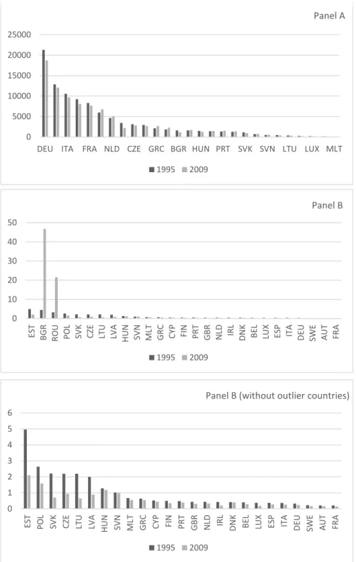
For a preliminary data analysis, Figures 1 and 2 show the amount of CO2
emissions at country (1995 and 2009) and sector (1995, 2002 and 2009) levels, respectively.
Performances of countries are rather heterogeneous (Figure 1). European
emissions (Panel A) show a decrease of almost 23% (or 268 thousand kilotons) between 1995 and 2009. During this period, 20 of 27 countries reduced their emissions; 5 of these (Germany, Italy, France, the United Kingdom and Poland) account for 70% of the total reduction (187 thousand kilotons). Luxembourg, Romania and Bulgaria are the top performers in relative terms, with reductions between 57 and 75.5% with respect to their 1995 levels. Among the 7 countries with emissions higher in 2009 than in 1995, Spain (+3.4%) and Austria (+4.3%) are the most important. In terms of emission intensity of value added (computed as the ratio of CO2 emissions produced per unit of value added)
we note that in 2009, this indicator increased by 941% and 561% in Bulgaria and Romania, respectively, while changes relative to other countries are less remarkable. There are several reasons for this difference. For example, the crisis might have affected these growing economies more, causing a reduction of value added in 2009 that was greater than the reduction in CO2 emissions. Another version of Panel B (without the
outlier countries) shows that, in general, emission intensity was higher in the eastern European countries in 1995 but significantly decreased in 2009. Emission intensities of southern and northern EU countries do not show a remarkable variation between these two years.
13 0 5000 10000 15000 20000 25000
DEU ITA FRA NLD CZE GRC BGR HUN PRT SVK SVN LTU LUX MLT
Panel A 1995 2009 0 10 20 30 40 50 ES T BGR RO U PO L SV K CZE LTU LVA HUN SVN ML T G R C CY P FIN PRT GBR NLD IRL DN K BE L LUX ESP ITA DEU SWE AUT FRA Panel B 1995 2009 0 1 2 3 4 5 6 ES T PO L SV K CZE LTU LVA HUN SVN ML T G R C CY P FIN PRT GBR NLD IR L DN K BE L LUX ESP ITA DEU SWE AUT FRA Panel B (without outlier countries)
1995 2009
Figure 1 - CO2 emissions (Panel A) and CO2 emission intensity of value added (Panel B) at
14
Figure 2 refers to sectorial emission levels at the beginning of the study period (in 1995), in the middle (2002) and at the end (2009). Among the most polluting
activities are the production of basic metals and metal products, the manufacture of non-metallic minerals (such as ceramic, glass, and cement), the chemical sector and
activities related to coke and refined petroleum. Notwithstanding these initial
performances, the following sectors reduced their environmental impact over time: the metal sector, the non-metallic minerals sector and the chemical sector. Relatively lower CO2 emissions are produced by the electrical equipment and other machinery sectors,
the wood sector and the production of leather sector.
Regarding the emission intensity of value added (panel B of figure 2), we find that the first four pollutants in Panel A are also the top four sectors for emission intensity. Moreover, we note that with respect to 1995, emission intensity increased in 2002, particularly for the manufacturing of coke and petroleum and the production of non-metallic minerals. Emission intensity in 2009 is decreased compared to both the
A 0 2000 4000 6000 8000 10000 12000 Panel A 1995 2002 2009 0 1 2 3 4 5 6 7 8 9 10 Panel B 1995 2002 2009
Figure 2 - CO2 emissions (Panel A) and CO2 emission intensity of value added (Panel B) at
15
beginning and the end of the study period due to the negative variation of value added in that year.
Nevertheless, to properly interpret all this information, we must also consider the tendencies of the value added of the manufacturing sector. In fact, at least part of the decrease in emissions might be due to minor manufacturing activity, which in turn may be related to an ongoing structural change in the European economy towards the services sector and the latest economic crisis that involved the European industry.
Figure 1 - Trends in environmental productivity. 1995=100. Selected EU27 countries. Source of data: WIOD
Figure 3 depicts the evolution of environmental productivity (EP) in selected EU27 countries. Environmental productivity has experienced a greater increase in the United Kingdom, which also started from a higher value in 1997, showing a persistent positive trend. In contrast, among the continental countries, there has been a decrease in EP for the last part of the 1990s and the first years of the 2000s. However, since 2003, the variation of EP has been steadily positive. The positive trend signals that there has been an actual improvement in terms of environmental impact; therefore, we also check the trend of value added. The levels measured in the last year of the time series (2009) are in the range between 1 and 2.5 euros of value added per kiloton of CO2 emissions.
As for the average growth rates of trade flows, the data are provided by the OECD (OECD-STAN Bilateral Trade Database in Goods), which also applies the ISIC Rev. 3 industrial classification. Bulgaria, Luxembourg and Slovakia have no trade data available for any of the industrial sectors analysed; hence, in the section that considers the regression of the trade variable, we refer to a dataset of 330 total observations.
As a measure of the technological change dimension, we choose patent
applications because this is an indicator of innovation processes. We do not discriminate between environmental and non-environmental technologies because innovation is intended in a broader sense, akin to the definition of sustainable innovation (SI) in Ketata et al. (2015). In contrast to environmental innovation (Rennings, 2000), SI is a
50 70 90 110 130 150 170 190 210 1995 1996 1997 1998 1999 2000 2001 2002 2003 2004 2005 2006 2007 2008 2009
16
more inclusive concept that not only involves the environmental dimension but also actual social issues and the needs of future generations (Ketata et al., 2015). The patent variable refers to the growth rates of patent stock for each manufacturing sector from 1977 to 2009. To obtain this dataset, we use yearly data on patent applications to the European Patent Office (EPO), which are provided by the OECD. The total
observations are 310, since much of the data on Eastern Europe are missing
(particularly for countries such as Estonia, Latvia, Lithuania, Romania and Slovakia). Detailed information on the computation of the stock of patents and its growth rate are presented in the Appendix.
Finally, data on the number of active firms are retrieved from Eurostat. Unfortunately, data were available only for 1997 and later.
17
5 Results
5.1 β-Convergence
Table 2 reports the coefficients estimated using a parsimonious regression model to test the existence of absolute convergence (column 1) and convergence conditional to sector and country fixed effects. Table 3 present the results of the full model as framed in equation (5) while different robustness checks are shown in tables 4 and 5.
The specification in column 1 shows a negative and significant β with a value of -0.026, which suggests the presence of absolute (unconditional) convergence. The significance of log EP (1995) is robust to the introduction of country and sector fixed effects, although the magnitude of the conditional convergence appears lower. When we narrow the analysis to focus on either EU15 or non-EU15 countries, we find that while the result holds for non-EU15 countries (column 4), the coefficient of log EP (1995) is not significant (column 5). One interpretation of this result is that the oldest EU countries might have achieved similar environmental productivities performances.
Table 2 - Basic model and EU15 and non-EU15 subsamples
Basic model EU15 Non-EU15
(1) (2) (3) (4) (5) Log EP (1995) −0,026*** (0,004) −0,008** (0,003) −0,021*** (0,005) −0,003 (0,004) −0,031*** (0,004)
Country fixed effects no yes yes no no
Sector fixed effects no no yes no no
Observations 362 362 362 197 165
R2 0,23 0,80 0,84 0,00 0,31
Notes: for each column, standard errors of regression coefficients appear in parenthesis. Significance level: * p < 0,10, ** p < 0,05, *** p < 0,01.
18
Table 3 - Covariate specification of the model
Dependent var: (1) (2) (3) (4) (5) Growth of EP Log EP (1995) -0.0129*** -0.0129*** -0.0129*** -0.0141*** -0.0137*** (0.00392) (0.00392) (0.00392) (0.00440) (0.00436) Trade openness 1.266*** 1.266*** 1.266*** 1.268*** 1.255*** (0.203) (0.203) (0.203) (0.231) (0.225) Patent stock -0.0928 (0.0954) -0.0928 (0.0954) -0.0928 (0.0954) -0.103 (0.115) -0.103 (0.114) ETS 0.000233 (0.0238) 0.00435 (0.0244) 0.00524 (0.0245)
Δ Sectorial n. of firms 2.90e-06
(1.67e-05) 1.25e-06 (1.55e-05) Δ Sectorial share of value added -0.0188* (0.0111)
Sector FE Yes Yes Yes Yes Yes
Observations 275 275 275 237 236
R-squared 0.359 0.359 0.359 0.357 0.364
Robust standard errors appear in parentheses *** p<0.01, ** p<0.05, * p<0.1
Table 3 presents the regression results for different specifications and for the full
specification (column 5). While convergence holds, environmental productivity appears to be positively influenced by trade openness (column 1), which exerts its effect by increasing value added. The coefficient is positive (1.266) and statistically significant at the 1% level.
The second column in Table 3 refers to the regression that adds the technology dimension. The variable included in the model is the growth of patent stock, as
presented in section 3. The coefficients relative to initial EP levels (β) and the trade dimension (γ) hold in magnitude and significance with respect to those obtained in the previous specification. Examining the coefficient of the growth of patent stock (δ), we note that the coefficient is negative but not significant, which means that technology does not have a relevant effect on the EP convergence process in Europe. Although this result may appear counterintuitive, it is worth noting that there might be very large disparities in terms of innovation capacities across sectors and countries, due to factors such as different levels of availability of resources to invest in R&D projects13. This
means that countries with higher levels of technological development are building new knowledge from a higher starting point compared to countries that are laggards in terms of innovation capacity. Therefore, technology might not be a significant factor in the convergence of environmental performances.
13For instance, Gilli, Mazzanti and Nicolli (2013) note that, typically, northern EU countries (e.g.,
Germany and Sweden) show a high degree of innovative capability (with a high share of eco-innovations) and have a longer tradition of environmental protection oriented policies than southern and eastern EU countries (e.g., Italy). Therefore, the effect of technological change as a driver of improved environmental productivity might not fully emerge at the EU aggregate level.
19
In the following, we consider the inclusion of a dummy variable relative to the EU Emission Trading Scheme (column 3). The coefficient is not significant, signalling that the introduction of this policy to reduce GHG emissions did not affect the
convergence of environmental productivity. However, our data includes only part of the first phase of the introduction of the system and the emission limits in 2005 were not stringent, which would have hindered any possible effect on EP (Abrell, Ndoye Faye and Zachmann, 2010).
Column 4 shows that inclusion of an additional independent variable (the variation of the number of firms per sector) does not significantly affect the process of convergence of environmental productivity. However, we found that the variation of the sectorial share of value added, shown in the full model of column 5, is significant with a negative coefficient. Thus, variation of the industry share of value added tends to
decrease the value of the environmental productivity indicator.
Following Rodrik (2013), we conduct some additional tests using different sub-samples to check for the robustness of our model. The results for the robustness check are summarized in table 4.
Table 4 - Robustness check of the full model in table 3, column 5
Dependent var: (1) (2) (3) (4) (5)
Growth of EP Euro Non-euro Interquantile range 50% highest EP 50% lowest EP
Log EP (1995) -0.0188** -0.0212*** -0.0156*** -0.0174*** -0.00635** (0.00772) (0.00561) (0.00439) (0.00626) (0.00270) Trade openness -0.489 1.398*** 1.301*** 1.048*** -0.0442 (0.316) (0.221) (0.235) (0.346) (0.143) Patent stock 0.188 -0.277* -0.148 -0.166 -0.203* (0.120) (0.162) (0.120) (0.147) (0.110) ETS -0.000251 -0.0386 0.00779 -0.0293 0.00319 (0.0185) (0.0585) (0.0246) (0.0444) (0.0101)
Δ Sectorial n. of firms 8.25e-06 5.28e-05** 2.42e-06 1.27e-05 1.15e-05
(1.99e-05) (2.63e-05) (1.72e-05) (2.23e-05) (7.62e-06)
Δ Sectorial share of value added -0.00638 (0.00515) -0.0723** (0.0359) -0.0229 (0.0155) -0.0499* (0.0272) -0.00189 (0.00418)
Sector FE Yes Yes Yes Yes Yes
Observations 147 89 214 106 130
R-squared 0.212 0.582 0.380 0.329 0.320
Robust standard errors appear in parentheses *** p<0.01, ** p<0.05, * p<0.1
First, we divided the sample based on whether countries adopted the euro (column 1 and column 2). The relation with log EP (1995) is statistically significant in both cases but note that, first, the coefficient of the initial level of EP has a slightly higher magnitude for non-euro countries and second, trade appears to significantly influence the convergence process only for this group of member states. The variation of the sectorial number of firms and of the sectorial share of value added is significant for the non-euro countries. Thus, in this subsample, factors related to the structure of the manufacturing sector appear to be relatively more important for environmental
20
To test if the regression results are sensitive to the presence of outliers, regressions are also run excluding the extreme observations of ΔEP and considering only values within the interquartile range (i.e., between the 25th and the 75th percentiles). 215 observations belong to this subsample (column 3). Significance of the convergence process holds and the coefficient of log EP (1995) is higher in magnitude with respect to those presented in table 3. In addition, trade maintains its significance and magnitude.
The same occurs with the sub-sample that includes only 50% of the highest value observations of EP (column 4). In contrast, when considering the lowest value observations of EP (column 5), the coefficient of the initial level of environmental productivity remains significant but is remarkably lower compared to the other
subsamples. Moreover, trade in this subgroup does not seem to significantly affect the ongoing convergence process of environmental productivity.
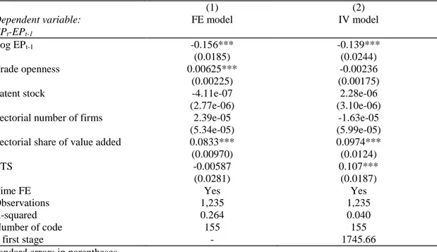
As a further robustness check and to mitigate the economic effects of the crises in 2009 and other cyclical factors, we also considered a panel version of our dataset, which can be interpreted as an assessment of short term economic effects on the relation. The results are summarized in table 5 where we considered both a fixed effect model and a simple instrumental variable model. In alignment with Reed (2015), we chose the second lag of the logarithm of environmental productivity as an instrument for the lagged logarithm of environmental productivity. The dependent variable is the annual variation of environmental productivity. In this case, (panel) convergence is computed using the lagged logarithm of environmental productivity instead of the initial level. All the other regressors are included in levels. β-convergence holds in the short term for both specifications. Trade openness remains positive and significant in column 1 but not in the instrumental variable model in column 2. The magnitude of
convergence is greater in the short term than in the long term (see table 4). In addition, the share of industry value added appears to exert a significant effect on environmental productivity; particularly in the short run, an increase in the share of value added positively affects the dependent variable.
21
Table 5 - Fixed effects and instrumental variable models
(1) (2) Dependent variable: EPt-EPt-1 FE model IV model Log EPt-1 -0.156*** -0.139*** (0.0185) (0.0244) Trade openness 0.00625*** -0.00236 (0.00225) (0.00175)
Patent stock -4.11e-07 2.28e-06
(2.77e-06) (3.10e-06)
Sectorial number of firms 2.39e-05 -1.63e-05
(5.34e-05) (5.99e-05)
Sectorial share of value added 0.0833***
(0.00970)
0.0974*** (0.0124)
ETS -0.00587 0.107***
(0.0281) (0.0187)
Time FE Yes Yes
Observations 1,235 1,235
R-squared 0.264 0.040
Number of code 155 155
F first stage - 1745.66
Standard errors in parentheses *** p<0.01, ** p<0.05, * p<0.1
To summarize, our first set of results highlight that i) there is a tendency of absolute convergence in terms of environmental productivity in the European industrial sectors between 1995 and 2009; ii) considering a conditional convergence perspective, the process is positively influenced by a country’s trade openness and negatively influenced by the sectorial share of value added.
Considering the additional regressions for different subsamples, we find that the fundamental hypothesis is verified. Indeed, when considering leader and laggard
countries separately, the coefficient β is negative and statistically robust for this last group. Finally, we also find evidence that convergence persists in the short run and is robust to economic shocks and business cycle dynamics.
5.2 σ-convergence
The final part of this analysis is focused on σ-convergence (figure 3). Thus far, we have supported the existence of convergence in the growth rates of environmental productivity. In other words, we found support for the hypothesis that laggard countries, in terms of environmental productivity, are improving their performance at a higher rate than countries that already show positive performance in EP.
Recall from section 3 that regarding σ-convergence, the aim is to assess if the speed at which laggard countries are improving is fast enough to close the gap between leaders and laggards.
22
As noted in figure 3, the majority of the sectors show increasing variability in environmental productivity. For certain sectors (e.g., machinery and equipment in Panel A and electrical equipment in Panel B), the gap in environmental performances among EU27 countries is increasing. This suggests that although laggard countries are
improving their EP at a faster rate than leader countries, the speed of improvement for these sectors is not sufficient to close the existing divide. However, for other sectors, such as coke and petroleum and wood production in Panel A and leather, textiles and food and beverages in Panel B, there is evidence of a reduction in the variability of the EP indicator over time. For these sectors, the convergence of environmental
performances, on average, begins around the beginning of the 2000s. However, since
20 40 60 80 100 120 140 160 180 200 1995 1996 1997 1998 1999 2000 2001 2002 2003 2004 2005 2006 2007 2008 2009 Panel A
Wood Manufacturing n.e.c. Machinery & Equip.
Metals Tranport equip. Chemicals
Coke & Petroleum
0 50 100 150 200 250 300 350 400 40 60 80 100 120 140 1995 1996 1997 1998 1999 2000 2001 2002 2003 2004 2005 2006 2007 2008 2009 Panel B
Food & Beverages Rubber & Plastic Leather
Paper Textile Non metallic minerals
Electrical equip.
Figure 3 - Change in the EP coefficient of variation. 1995-2009; 1995=100. Sectorial level. EU27. In Panel B, the electrical equipment sector is represented on the right axis.
23
the evidence for such dynamics remains limited in the sample, the hypothesis of a reduction of the gap between laggard and leader countries is not fully supported.
This result may be a signal that although environmental performances and commitments to the decarbonization of the economy are improving in EU laggard member states, the effort cannot yet fully compensate for the gap between laggard and leader countries. Finally, we note that the presence of a β-convergence and the
simultaneous absence of an σ-convergence are compatible, according to Stegman and McKibbin (2005) and Rodrik, 2013. This situation may be due to unobserved factors that influence the growth of environmental productivity.
6 Conclusions
The aim of this study is to offer a new and different perspective on the environmental performances of the European manufacturing sector. Specifically, this analysis is
focused on detecting, describing and testing the relevance of the convergence process of environmental productivity across the manufacturing sectors of the European countries. Both β-convergence and σ-convergence are considered; the former informs the
existence of a catching-up process for which laggard countries, in terms of sectorial environmental productivity, are performing better (i.e., increasing more) than leader countries (i.e., countries that already show good environmental productivity
performance).
σ-convergence relates to the sectorial variability of environmental productivity among sectors in different countries; if variability decreases over time, then the gap between laggard and leader countries, in terms of environmental performances, is becoming smaller.
The results support the hypothesis that an ongoing β-convergence process exists, which implies that the environmental productivity of manufacturing sectors in laggard countries is growing faster than the environmental productivity of manufacturing sectors in leader countries.
In addition, the inclusion of other relevant variables in the model signals that aspects such as trade openness and changes in the sectorial share of value added have relevant effects. Specifically, trade openness has a positive effect on the growth of
environmental productivity while fluctuations in value added reduce environmental productivity. Notwithstanding the support for β-convergence, there is no evidence of an ongoing process of σ-convergence, indicating that the discrepancy in EU environmental performances is not reducing over the considered period.
Jointly, these results might indicate that although laggard countries are exerting greater efforts towards improving their environmental performances than leader
countries, the gap between these two groups is widening; the increase in EP for laggards is not sufficient to compensate for their distance from the leaders.
As noted in section 5, technology does not appear to be a significant factor in increasing the rate of environmental productivity. This result, which might be surprising
24
at first, can be explained by the fact that within the EU, countries have very different levels of technological knowledge bases and diverse institutional and cultural
conditions. From a policy perspective, this implies support for the term “two-speed Europe” and underlines how policies oriented towards the increase of a country’s technological knowledge base might be essential not only for the well-known
advantages in terms of economic growth but also for the improvement in environmental performances of the overall Union.
Acknowledgements
The authors acknowledge financial support of the Europen research project “Green.eu – European Global transition network on Eco-innovation, Green Economy and
25
References
Abrell, J., Ndoye Faye, A. & Zachmann, G. (2011). Assessing the impact of the EU ETS using firm level data. Bruegel Working Paper 2011/08.
Aldy, J.E. (2006). Per Capita Carbon Dioxide Emissions: Convergence or Divergence?
Environmental and Resource Economics, 33(4), 533-555. DOI 10.1007/s10640-005-6160-x
Barassi, M.R., Cole, M.A. & Elliott, R.J.R. (2008). Stochastic Divergence or Convergence of Per Capita Carbon Dioxide Emissions: Re-examining the Evidence. Environmental and
Resource Economics, 40(1), 121- 137. DOI 10.1007/s10640-007-9144-1
Barro, R.J. & Sala-i-Martin, X. (1991). Convergence across States and Regions. Brookings
Papers on Economic Activity, 1, 107-182.
Bernard, A.B. & Durlauf, S.N. (1995). Convergence in international output. Journal of applied
econometrics, 10(2), 97-108. DOI 10.1002/jae.3950100202
Bernard, A.B. & Durlauf, S.N. (1996). Interpreting tests of the convergence hypothesis. Journal
of Econometrics, 71, 161-173. DOI 10.1016/0304-4076(94)01699-2
Calcagnini, G., Giombini, G. & Travaglini, G. (2016). Modelling energy intensity, pollution per capita and productivity in Italy: A structural VAR approach. Renewable and Sustainable
Energy Reviews, 59, 1482-1492. DOI 10.1016/j.rser.2016.01.039
Carson, R. T. (2009). The environmental Kuznets curve: seeking empirical regularity and theoretical structure. Review of Environmental Economics and Policy, 4(1), 3-23.
Cole, M.A., Elliott, R.J.R. & Shimamoto K. (2005). Industrial characteristics, environmental regulations and air pollution: an analysis of the UK manufacturing sector. Journal of
Environmental Economics and Management, 50(1), 121-143. DOI 10.1016/j.jeem.2004.08.001
Dietzenbacher, E., Los, B., Stehrer, R., Timmer, M. & De Vries, G. (2013). The Construction of World Input-Output Tables in the WIOD Project. Economic Systems Research, 25 (1), 71-98. DOI 10.1080/09535314.2012.761180
Dinda, S. (2004). Environmental Kuznets Curve Hypothesis: A Survey. Ecological Economics, 49, 431-455. DOI 10.1016/j.ecolecon.2004.02.011
EEA - European Environment Agency (2014). Resource-efficient green economy and EU policies
(EEA Report 2/2014). Luxembourg, Publications Office of the European Union. DOI
10.2800/18514
EEA - European Environment Agency (2015). Annual European Union greenhouse gas inventory
1990–2013 and inventory report 2015 (EEA Technical report 19/2015). Luxembourg.
Publications Office of the European Union. DOI 10.2800/274962
European Commission (2014). For a European Industrial Renaissance. COM 14/2.
Ezcurra, R. (2007). Is there cross-country convergence in carbon dioxide emissions? Energy
Policy, 35(2), 1363-1372. DOI 10.1016/j.enpol.2006.04.006
Gilli, M., Mazzanti, M., & Nicolli, F. (2013). Sustainability and competitiveness in evolutionary perspectives: Environmental innovations, structural change and economic dynamics in the EU. The Journal of Socio-Economics, 45, 204-215.
26
Herrerias, M.J. (2013). The environmental convergence hypothesis: Carbon dioxide emissions according to the source of energy, Energy Policy, 61, 1140-1150. DOI 10.1016/j.enpol.2013.06.120
Islam, N. (2003). What have we learnt from the convergence debate? Journal of Economic
Surveys, 17(3), 309-362. DOI 10.1111/1467-6419.00197
Ketata, I., Sofka, W., & Grimpe, C. (2015). The role of internal capabilities and firms' environment for sustainable innovation: evidence for Germany. R&D Management, 45(1), 60-75.
Kijima, M., Nishide, K., & Ohyama, A. (2010). Economic models for the environmental Kuznets curve: A survey. Journal of Economic Dynamics and Control, 34(7), 1187-1201.
Lee, C.C. & Chang, C.P. (2008). New evidence on the convergence of per capita carbon dioxide emissions from panel seemingly unrelated regressions augmented Dickey-Fuller tests.
Energy, 33(9), 1468-1475. DOI 10.1016/j.energy.2008.05.002
Lee, K., Pesaran, M.H. & Smith, R.P. (1997). Growth and convergence in a multi-country empirical stochastic Solow model. Journal of applied Econometrics, 12(4), 357-392. DOI 10.1002/(SICI)1099-1255(199707)12:4<357::AID-JAE441>3.0.CO;2-T
Marin, G. (2012). Closing the gap? Dynamic analyses of emission efficiency and sector productivity in Europe. IMT Lucca EIC Working Paper Series 02.
Martinez-Zarzoso, I., Bengochea-Morancho, A. & Morales-Lage, R. (2007). The impact of population on CO2 emissions: evidence from European countries. Environmental and
Resource Economics, 38(4), 497-512. DOI 10.1007/s10640-007-9096-5
Panopoulou, E. & Pantelidis, T. (2009). Club Convergence in Carbon Dioxide Emissions.
Environmental and Resource Economics, 44(1), 47-70. DOI 10.1007/s10640-008-9260-6
Phillips, P.C.B. & Sul, D. (2007). Transition Modeling and Econometric Convergence Tests.
Econometrica, 75(6), 1771-1855. DOI 10.1111/j.1468-0262.2007.00811.x
Reed, W. R. (2015). On the practice of lagging variables to avoid simultaneity. Oxford Bulletin of Economics and Statistics, 77(6), 897-905.
Repetto, R. (1990). Environmental Productivity and Why It Is So Important. Challenge, 33(5), 33-38. DOI 10.1080/05775132.1990.11471458
Robbins, A. (2016). How to understand the results of the climate change summit: Conference of Parties21 (COP21) Paris 2015. Journal of Public Health Policy, 1-4. DOI 10.1057/jphp.2015.47
Rodrik, D. (2013). Unconditional Convergence in Manufacturing. The Quarterly Journal of
Economics, 128(1), 165-204. DOI 10.1093/qje/qjs047
Romero-Avila, D. (2008). Convergence in carbon dioxide emissions among industrialised countries revisited. Energy Economics, 30(5), 2265-2282. DOI 10.1016/j.eneco.2007.06.003 Schmoch, U., Laville, F., Patel, P. & Frietsch, R. (2003). Linking Technology Areas to Industrial
Sectors. Final Report to the European Commission, DG Research.
Stegman, A. & McKibbin, W.J. (2005). Convergence and Per Capita Carbon Emission, Brookings
Discussion Papers in International Economics No. 167.
Strazicich, M.C. & List, J.A. (2003). Are CO2 Emission Levels Converging Among Industrial Countries? Environmental and Resource Economics, 24(3), 263-271. DOI 10.1023/A:1022910701857
27
UNFCCC - United Nations Framework Convention on Climate Change (2015), Adoption of the
Paris Agreement. Conference of the Parties, Twenty-first session, from 30 November to 11
December 2015, Paris.
Weina, D., Gilli, M., Mazzanti, M. & Nicolli F. (2016). Green inventions and greenhouse gas emission dynamics: a close examination of provincial Italian data. Environmental
Economics and Policy Studies, 18(2), 247-263. DOI 10.1007/s10018-015-0126-1
Westerlund, J. & Basher, S.A. (2007). Testing for Convergence in Carbon Dioxide Emissions Using a Century of Panel Data. MPRA Paper No. 3262.
York, R., Rosa, E.A. & Dietz, T. (2003). STIRPAT, IPAT and ImPACT: analytic tools for unpacking the driving forces of environmental impacts. Ecological Economics, 46(3), 351-265. DOI 10.1016/S0921-8009(03)00188-5
28
Appendix
To obtain the patent stock for each industrial sector, we use data mined from the OECD database for patent applications. We selected the total number of patent applications to the European Patent Office (EPO) by the applicant’s country of residence and by the patent class of the application (according to the International Patent Classification). The data covered the period 1977-2009.
Prior to calculating patent stock and its annual growth rate, we needed to match the IPC classes to the ISIC rev.3 classification. We did this using the correspondence table originally developed by Schmoch et al. (2003).
We computed the patent stock so that it considers both the annual flow of new patents and the stock of existing patents, depreciated to account for technological obsolescence in alignment with Popp et al (2011). In addition, we applied another analysis using patent data stock as in Weina et al (2016) and Franco and Marin (2017). The stock is obtained as follows:
0 , , ) 1 ( ) ( , , (1 ) 2 1 s s t c i s s t i c e e PAT KStock where β1 is the rate of knowledge obsolescence (set equal to 0.1) and β2 is the rate of
knowledge diffusion (set equal to 0.25)14.
Eventually, the compound annual growth rate from 1995 to 2009 is calculated in the same manner as the other variables in the study:
1 1995 2009 1 1995 , , 2009 , , , i c i c i c KStock KStock TECH