A
A
l
l
m
m
a
a
M
M
a
a
t
t
e
e
r
r
S
S
t
t
u
u
d
d
i
i
o
o
r
r
u
u
m
m
–
–
U
U
n
n
i
i
v
v
e
e
r
r
s
s
i
i
t
t
à
à
d
d
i
i
B
B
o
o
l
l
o
o
g
g
n
n
a
a
DOTTORATO DI RICERCA IN
MODELLISTICA FISICA PER LA PROTEZIONE
DELL’AMBIENTE
Ciclo XXII
Settore/i scientifico-disciplinare/i di afferenza: FIS/06
TITOLO TESI
Analisi della dinamica e composizione chimica del
particolato atmosferico mediante un modello alla
mesoscala.
Presentata da: PAOLO STOCCHI
Coordinatore Dottorato
Relatore
ROLANDO RIZZI
STEFANO TIBALDI
Abstract
The vertical profile of aerosol in the planetary boundary layer of the Milan urban area is studied in terms of its development and chemical composition in a high-resolution modelling framework. The period of study spans a week in summer of 2007 (12-18 July), when continuous LIDAR measurements and a limited set of balloon profiles were collected in the frame of the ASI/QUITSAT project.
LIDAR observations show a diurnal development of an aerosol plume that lifts early morning surface emissions to the top of the boundary layer, reaching maximum concentration around midday. Mountain breeze from Alps clean the bottom of the aerosol layer, typically leaving a residual layer at around 1500-2000 m which may survive for several days. During the last two days under analysis, a dust layer transported from Sahara reaches the upper layers of Milan area and affects the aerosol vertical distribution in the boundary layer.
Simulation from the MM5/CHIMERE modelling system, carried out at 1 km horizontal resolution, qualitatively reproduced the general features of the Milan aerosol layer observed with LIDAR, including the rise and fall of the aersol plume, the residual layer in altitude and the Saharan dust event. The simulation highlighted the importance of nitrates and secondary organics in its composition. Several sensitivity tests showed that main driving factors leading to the dominance of nitrates in the plume are temperature and gas absorption process.
A modelling study turn to the analysis of the vertical aerosol profiles distribution and knowledge of the characterization of the PM at a site near the city of Milan is performed using a model system composed by a meteorological model MM5 (V3-6), the mesoscale model from PSU/NCAR and a Chemical Transport Model (CTM) CHIMERE to simulate the vertical aerosol profile. LiDAR
continuous observations and balloon profiles collected during two intensive campaigns in summer 2007 and in winter 2008 in the frame of the ASI/QUITSAT project have been used to perform comparisons in order to evaluate the ability of the aerosol chemistry transport model CHIMERE to simulate the aerosols dynamics and compositions in this area.
The comparisons of model aerosols with measurements are carried out over a full time period between 12 July 2007 and 18 July 2007.
The comparisons demonstrate the ability of the model to reproduce correctly the aerosol vertical distributions and their temporal variability. As detected by the LiDAR, the model during the period considered, predicts a diurnal development of a plume during the morning and a clearing during the afternoon, typically the plume reaches the top of the boundary layer around mid day, in this time CHIMERE produces highest concentrations in the upper levels as detected by LiDAR. The model, moreover can reproduce LiDAR observes enhancement aerosols concentrations above the boundary layer, attributing the phenomena to dust out intrusion. Another important information from the model analysis regard the composition , it predicts that a large part of the plume is composed by nitrate, in particular during 13 and 16 July 2007 , pointing to the model tendency to overestimates the nitrous component in the particular matter vertical structure . Sensitivity study carried out in this work show that there are a combination of different factor which determine the major nitrous composition of the “plume” observed and in particular humidity temperature and the absorption phenomena are the mainly candidate to explain the principal difference in composition simulated in the period object of this study , in particular , the CHIMERE model seems to be mostly sensitive to the absorption process.
Chapter 1
Air quality on the regional and local scale and in particular suspended particles are of great interest for society, because they affect human health, forests and other ecosystem (Roberts, 2003; WHO, 2005). Moreover particles play a key role in climate change (IPCC, 2007) since they affect the Earth’s radiative balance, directly by altering the scattering properties of the atmosphere, and indirectly by changing clouds properties (Rosenfeld et al., 2008). Increasing concentrations of anthropogenic aerosols may be partially counteracting the warming effects of greenhouse gases by an uncertain, but potentially large, amount. This in turn leads to large uncertainties in the sensitivity of climate to human perturbations and therefore also in the projections of future climate change [Penner, 2004; Andreae et al., 2005]. Various aerosol types (sulfate, carbonaceous aerosol, mineral dust, and sea salt) contribute to this effect on climate. These aerosols scatter and absorb incoming solar radiation increasing the planetary albedo (the direct effect) and they also enhance the albedo and extent of clouds by increasing the number of cloud droplets (the first indirect effect or Twomey effect) and by changing the precipitation efficiency of clouds (the second indirect effect or Albrecht effect). In order to study air quality and to gain information on aerosol physical and chemical characteristics, long-term particulate matter data have been collected in different kind of sites (e.g. Van Dingenen, 2004; Putaud et al., 2004). However, surface measurements are not sufficient to fully understand the pollutants dynamics and chemistry. Current Eulerian models are found to represent well the primary processes impacting the evolution of trace species in most cases though some exceptions may exist. For example, sub-grid-scale processes, such as concentrated power plant plumes, are treated only approximately. It is not apparent how much such approximations affect their results and the polices based upon those results. A significant weakness has been in how investigators have addressed, and communicated, such uncertainties. Studies found that major uncertainties are due to model inputs, e.g., emissions and meteorology, more so than the model itself. One of the primary weakness identified is in the modeling process, not the models.
Evaluation has been limited both due to data constraints. Seldom is there ample observational data to conduct a detailed model intercomparison using consistent data (e.g., the same emissions and meteorology). Further model advancement, and development of greater confidence in the use of models, is hampered by the lack of thorough evaluation and intercomparison. Model advances are seen in the use of new tools for extending the interpretation of model results, e.g., process and sensitivity analysis, modeling systems to facilitate their use, and extension of model capabilities, e.g., aerosol dynamics capabilities and sub-grid-scale representations. For a better understanding of pollutant evolution important efforts have been made to develop and improve three dimensional air quality models (Seigneur 2001; Zhang et al., 2004, 2006a, 2006b). Such models are now regarded as important instruments for monitoring, forecasting and planning of atmospheric environment as provided for the Directive 2008/50/CE. Several modelling studies focused on the Po Valley region, which is the most populated and industrialized area in Italy. There, favourable conditions for severe pollution episodes are often observed, due to prolonged hot and stagnant conditions during summer and frequent foggy days in autumn and winter (Silibello et al., 2007). These studies analyzed particulate matter and gas pollutant horizontal distribution comparing modelling results with ground-based observations (Martilli et al.; 2002; Baertsch-Ritter et al., 2003; Angelino et al,. 2007; Andreani et al., 2008) . Angelino et al. (2007) show results of a comparison between two chemistry-transport models (CTMs) CAMx and TCAM The models reproduce the yearly mean of PM10 with a RMSE around 30 ug/m3 and capture the frequency distribution of the daily mean concentrations even in the case of acute episodes, with the exception of a few winter episodes. The models are able to reproduce the observed decrease in nitrates and increase in sulphates from winter to summer and the greater sensitivity to temperature of nitrates compared to sulphates. Baertsch-Ritter et al. (2003) and Martilli et al. (2002) focused their attention on sensitivity study to characterize the VOC/NOx regime of the O3 production in the Milan area. A recent study (Andreani 2008), concluded that the high PM2.5 concentration in
advected by thermal wind toward the Alps as well around Milan area. A major role in aerosol formation is found to be played by HNO3 and NH3 most of the time.
In our study we focused our attention on the modelled vertical profile of the particulate matter (PM), because a good representation of its distribution and compositions is an important step for studies related to public health (Liu et al 2004), and because there is still a gap in its characterization in Po Valley (Baltensperger et al., 2002). We implemented an air quality modelling system at 1 Km resolution over Milan with detailed urban landuse in order to help interpretation of the vertical structure of aerosol in the planetary boundary layer as observed with balloon-borne and continuous lidar measurements. Data used in this study have been collected during an intensive summer campaign in the frame of the ASI/QUITSAT project.
The major issues of this work are:
o Comparisons in the Milan area between vertical structures of PM from a CTM and from Lidar Measurements ;
o Modelling approach and sensitivity studies to improve the knowledge of the characterization of the PM in this area .
Seven days from 12 July to 18 July 2007are chosen to this purpose, these correspond to typical clear sky and stable meteorological conditions, in free convection regime.
We have compared on a quality level the PM profile detected by the lidar for these continuous days in order to evaluate how better the CTM Chimere reproduce temporally and spatially the diurnal vertical distribution of the aerosol load detected by lidar , then we did some sensitivity test to give a modeling interpretation to the vertical distribution observed in the area object of the study .
The work has been organized as follows: chapter 2 presents an overview about the Meteorological and the Chemical Transport models used for this study , chapter 3 illustrates the case study ,the Lidar and balloon measurements and their application in this work, while chapter 4 describe the sensitivity analysis performed. Chapter 5 is devoted to the discussion of results and conclusions.
In this chapter a description of the two models used in this study will be made. We used a modelling system which consist of the MM5 meteorological model from PSU/NCAR and Chemistry-Transport Model (CTM) CHIMERE.
2.1 MM5 Meteorological model
The Chemical Transport Model (CTM) CHIMERE require several meteorological variables as input. In order to force chemical simulation at high resolution (1Km) we create the meteorological input using MM5 (V3-6), the mesoscale model from PSU/NCAR. This is a non-hydrostatic, primitive-equation model with a terrain-following vertical coordinate (Grell er al., 1994 and Dudhia, 1993). The model has multiple-nesting capabilities to improve the simulation over the area of interest. For this study we used a PBL parameterizations (non local Medium Range Forecast (MRF)) coupled with Noah Land Surface Model (LSM)
The MRF PBL scheme (Hong and Pan, 1996) is a first-order, non-local K scheme, based on the representation of a counter gradient term that account for the contributions from large-scale eddies. The PBL height is calculated based on the critical bulk Richardson number. The MRF scheme is designed to represent the turbulence due to large eddies within a well-mixed PBL, thus to properly describe a PBL under non local, mesoscale forcing (Ferretti and Raffaele, 2008).
The Naoh land surface model predicts soil moisture and temperature as well as canopy moisture and water equivalent snow depth at four soil layers with thickness from top to bottom of 7, 28,100, 255 cm (Chen and Dudhia 2001a). It uses soil and vegetation types in handling evapotraspiration. The dominant vegetation type in each grid is selected to represent the grid vegetation characteristics when the model horizontal grid resolution is larger than 1 km x 1 km. Other physical parameterization schemes are: the mixed-phase microphysics (Reisner et al., 1998), used to explicitly predict supercooled liquid water and to allow for slow melting of snow. The Rapid
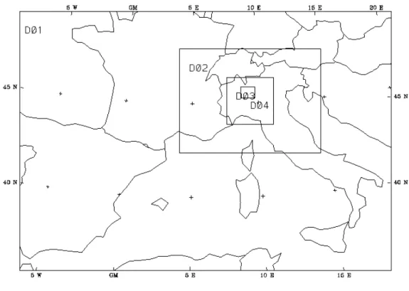
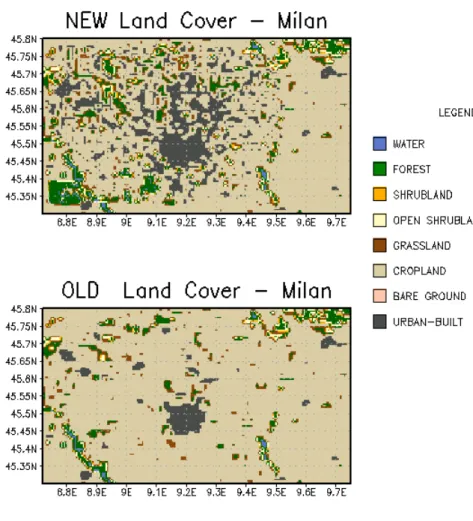
Radiative Transfert Model (RRTM) longwave scheme (Mlawer et al 1997), an highly accurate and efficient method for radiation transfer simulation. The cumulus parameterization is based on the Grell scheme which is based on rate of destabilization or quasi-equilibrium, simple single cloud scheme with updraft and downdraft fluxes and compensating motion determining heating/moistening profile. Shear effects on precipitation efficiency are considered (Grell et al. 1994). Four domains (Fig. 1) are used for this study: the mother domain has horizontal grid spacing of 27 Km and is centred at 43.0°N and 6.0°E. The first nested domain has a 9 Km grid spacing, covering the whole North of Italy. The second nest has a grid spacing of 3 Km, including the whole Po Valley. The last and finest domain has an horizontal grid of 1 km and it is centred over the city of Milan. We use an upgrade of the land-use for domain 4, characterized by a larger number of urban categories than the standard one available provided by USGS (Fig.2)
Figure 2: Upgrade of the land-use for domain 4 (top panel), characterized by a larger number of urban categories than the
standard one available provided by USGS (down panel)
2.2
MM5 basic equations
Atmospheric evolution is forecasted through the resolution of five equations (primitive equations). In detail, three motion equations (one for each wind component), one continuity equation and a thermodynamic equation are derived by the basic energy conservation laws concerning linear momentum, mass and energy. MM5 includes a multiple-nest capability and uses a sigma (σ) vertical coordinate, defined as
σ =
*
p
p
p
−
topwhere p is the pressure, ptop and psurf are the values of p at the top and on the surface and p*= psurf
- ptop. The equations governing a non-hydrostatic model are:
Tendency pressure (4) Momentum (x-component) (5) Momentum (y-component) (6) Momentum (z-component) (7)
Thermodynamics
(8)
Advection terms can be expanded as
(9)
Where
Equation (4) (tendency pressure) is obtained by the combination of the first law of thermodynamic with gas laws and continuity equation. Equations (5), (6), and (7) are the motion equations with regard to each wind component, while equation (8) supplies the thermodynamic balance. The advection terms are made explicit in equation (9).
The above equations are solved numerically by using finite differences: second-order centred finite differences represent the gradients, except for solved numerically by using the precipitation fall term, which uses a first-order upstream scheme for positive definiteness.
A second-order leapfrog time-step scheme is used for above equations, but some terms are handled using a time-splitting scheme. In the leapfrog scheme, the tendencies at time n are used to step the
variables from time n-1 to n+1. This is used for most of the right-hand terms (advection, Coriolis, buoyancy). A forward step is used for diffusion and microphysics, where the tendencies are calculated at time n-1 and used to step the variables from n-1 to n+1. When the time step is split, certain variables and tendencies are updated more frequently, because all sound waves u, v, w and p′ need to be updated each short step using the tendency terms, while the terms on the right are kept fixed. For sound waves there are usually four of these steps between n-1 and n+1, after which u, v, w and p′ are updated.
2.3 CHIMERE chemistry transport model
The chimere multi-scale model is primarly designed to produce daily forecast of ozone, aerosols and other pollutants and make long-term simulations for emission control scenarios. Chimere runs over a range of spatial scales from the regional scale to the urban scale with resolutions from 1-2 Km to 100 Km. The model is described in several articles (Schmidt et all., 2001; Vautard et al., 2003; Derognat et al., 2003; Bassagnet 2005). At the present application CHIMERE run at 1 Km of resolution over Milano area (Bicocca), boundary conditions are provided by a prior regional, large-scale simulation over Lombardia at 12 Km of resolution. The emissions that we use for this study come from CTN-ACE datasets inventory , with a original resolution of 10 km and then interpolated respectively at 12 Km and 1 Km. The vertical resolution of the fine-scale configuration is of 12 sigma levels extending up 500 hPa that cover the boundary layer and the lower part of the free troposphere. In this study we simulate 80 gaseous species and 7 aerosol chemical compounds, primary particle material (PPM), nitrate, sulfate, ammonium, biogenic secondary organic aerosol (SOA), anthropogenic and water. The gas-phase chemistry scheme include sulfur aqueous chemistry, secondary organic chemistry and heterogeneous chemistry of HONO (Aumont et al., 2003) and nitrate (Jacob, 2000).
2.3 Aerosol Module
The population of aerosol particles is represented using a sectional formulation, assuming discrete aerosol size sections and considering the particles of a given section as homogeneous in composition (internally mixed).The aerosol module accounts for both inorganic and organic species, of primary or secondary origin, such as, primary particulate matter (PPM), sulfates, nitrates, ammonium, secondary organic species (SOA) and water. PPM is composed of primary anthropogenic species such as elemental and organic carbon and crustal materials. Sulfate is produced from gaseous and aqueous oxidation of SO2). Nitric acid is produced in the gas phase by NOx oxidation, but also by heterogeneous reaction of N2O5 on the aerosol surface (Jacob, 2000). Issued directly from primary emissions, ammonia is converted into aerosol phase (mainly ammonium-nitrate and ammonium sulfate) by neutralization with nitric and sulfuric acids. Secondary organic aerosols are formed by condensation of biogenic and anthropogenic hydrocarbon oxidation products, they are partitioned between the aerosol and gas phase through a temperature-dependent partition coefficient (Pankow, 1994). A lookup table method, set up from the ISORROPIA equilibrium model (Nenes et al., 1998, 1999), is used to calculate concentrations at equilibrium for inorganic aerosols composed of sulfate, nitrate, ammonium, and water. Dynamical processes influencing aerosol population are also described. New particles are formed by nucleation of H2SO4 (Kulmala et al., 1998). Particles growth due to the coagulation and condensation of semivolatile species is also taken into account. The coagulation process applied for multicomponent system is calculated as in the work of Gelbard and Seinfeld [1980]. Aerosols can be removed by dry deposition (Seinfeld and Pandis, 1998) and wet removal (Guelle et al., 1998). Particles can be scavenged either by coagulation with cloud droplets or by precipitating drops. Moreover, particles act efficiently as cloud condensation nuclei to form new droplets.
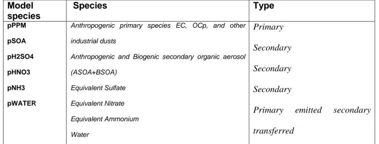
Model species Species Type pPPM pSOA pH2SO4 pHNO3 pNH3 pWATER
Anthropogenic primary species EC, OCp, and other industrial dusts
Anthropogenic and Biogenic secondary organic aerosol (ASOA+BSOA) Equivalent Sulfate Equivalent Nitrate Equivalent Ammonium Water Primary Secondary Secondary Secondary
Primary emitted secondary
transferred
Table 1: List of aerosol species
In the model, particles are composed of species listed in Table 9.2. Sulfate is formed through gaseous and aqueous oxidation of SO2. Nitric acid is produced in the gas phase by NOx oxidation. N2O5 is converted into nitric acid via heterogeneous pathways by oxidation on aqueous aerosols. Ammonia is a primary emitted base converted in the aerosol phase by neutralization with nitric and sulfuric acids. Ammonia, nitrate and sulfate exist in aqueous, gaseous and particulate phases in the model. As an example, in the particulate phase the model species pNH3 represents an equivalent ammonium as the sum of NH+4 ion, NH3 liquid, NH4NO3 solid, etc.
ISORROPIA models the sodium – ammonium – chloride – sulfate – nitrate – water aerosol system. Gas phase: NH3, HNO3, HCl, H2O
Liquid phase: NH4+ , Na+, H+, Cl-, NO3- , SO4- , HSO4-, OH-, H2O
Solid phase: (NH4)2SO4, NH4 HSO4, (NH4)3 H(SO4)2, NH4 NO3, NH4Cl, NaCl, NaNO3, NaHSO4,
Because sulfuric acid has a very low vapor pressure, it is reasonable to assume that it resides completely in the aerosol phase. The same assumption is made for sodium. Depending on the amount of sodium and ammonia, the sulfates can eitherbe completely or partially neutralized. There is also the possibility of completeneutralization of sulfuric acid by sodium alone. In each of these cases, the possible species are different. In order to determine which case is considered, two parameters are defined:
• RSO4 is known as the sulfate ratio, while RNa is known as the sodium ratio. The
concentrations are expressed in molar units. Based on the value of these two ratios, four types of aerosols are defined:
• Sulfate rich (free acid): This is when RSO4< 1. The sulfates are in abundance and part of it
is in the form of free sulfuric acid. In this case, there is always a liquid phase, because sulfuric acid is extremely hygroscopic (i.e., DRH is 0%).
• Sulfate rich (non free acid): This is when 1 ≤ RSO4 < 2. There is enough ammonia and
sodium to partially (but not fully) neutralize the sulfates. The sulfates are a mixture of bisulfates and sulfates, the ratio of which is determined by thermodynamic equilibrium. • Sulfate poor, Sodium poor: RSO4≥ 2; RNa < 2. There is enough ammonia and sodium to
fully neutralize the sulfates, but sodium is not enough to neutralize sulfates by itself. In this case, excess ammonia can react with the other species (HNO3, HCl) to form volatile salts. • Sulfate poor, Sodium rich: RSO4 ≥ 2; RNa > 2. There is enough sodium to fully neutralize the
(HNO3,HCl) to form salts, while no ammonium sulfate is formed (since all sulfates have
been neutralized with sodium).
Inputs needed by ISORROPIA are the total concentrations of Na, NH3, HNO3, HCl, and H2SO4
together with the ambient relative humidity and temperature. Then, based on the sulfate and sodium ratios, and the relative humidity, the appropriate subset of equilibrium equations (which correspond to the possible species for the conditions specified), together with mass conservation, electroneutrality and Equations (10) and (11) are solved to yield the equilibrium concentrations.
Chapter 3
a
w=RH (10)
The ambient relative humidity can be assumed to be uninfluenced by the deliquescence of aerosol particles because of the large amount of water vapor in the atmosphere .Under this assumption, and by neglecting the Kelvin effect, phase equilibrium between gas and aerosols gives that the water activity, aw, is equal to the ambient relative humidity where RH is expressed on a fractional (0–1) scale.
W=∑
i(11)
Mi s the molar concentration of species i in the air (mol m−3air), moi aw is the molality of an aqueous
solution of species i with the same water activity as the multicomponent solution and W is the mass concentration of aerosol water in the air (kg m−3 air)
In this chapter a description of the models configuration will be made with a brief introduction to Lidar and balloon data used in this work, emphasizing the attention on Lidar application and important comparisons with models results .
3.1 MM5 Model Setup and MRF scheme
Meteorological simulation was obtained from PSU/NCAR mesoscale model (MM5, v3 r3-6), a three-dimensional non-hydrostatic prognostic model, with four dimensional data assimilation (FDDA). Four nested domains were selected (chapter 2, Fig.1 ), which essentially covered Europe (D1, 27 km resolution), the Italy (D2, 9km), the north Italy (D3, 3 km) and the Milan urban area (D4, 1 km). Two way nesting approach was used; the vertical resolution was of 33 ϭ-layers with the upper boundary fixed at 100 hPa. The PBL parameterizations utilized is MRF (non local Medium Range Forecast (MRF)) coupled with Noah Land Surface Model (LSM) . MRF is non-local, first order closure PBL scheme which consist of two regimes: a stable one based on non local K-type closure theory and a free convection regime which takes the contributions from large-scale eddies into account in the local, vertical mixing process throughout the PBL introducing the effect of entrainment zone at the top of the PBL to mixing process. The transfer of heat follows the one dimensional simple diffusion equation as the flux is linearly proportional to the temperature gradient. The PBL height diagnosis is based on the bulk Richardson number (Rib); according to the literature a critical Rib of 0.22 was used for unstable conditions and a critical value of 0.33 in stable situations.
For this study we run Chimere at 1 Km of resolution over Milano area , boundary conditions came from CHIMERE previous runs over Pianura Padana at 12 Km of resolution. The emissions that we use for this study come from CTN-ACE inventory at resolution of 10 km and then interpolated respectively at 12 Km and 1 Km. Vertical resolution is of 12 sigma levels extending up 500 hPa that cover the boundary layer and the lower part of the free troposphere. In this study we simulate 80 gaseous species and 7 aerosol chemical compounds, primary particle material (PPM), nitrate, sulfate, ammonium, biogenic secondary organic aerosol (SOA), anthropogenic and water. CHIMERE has a sectional aerosol module with six diameter bins ranging between 10 nm and 40 µm with a geometric increase of bin bounds.
3.3 Observation and Tecniques: Lidar- Data and Application
Experimental data used in this study come from an automated lidar (Vaisala LD 40 ceilometer) and an Optical Particicle Counter (OPC) installed aboard a tethered balloon. The lidar used is able to countinuously (h24) collect backscattering profiles, with a spatial resolution of 7,5 m, and an averaging time of 15s. To improve the signal-to-noise ratio, integration over 15 minutes was performed. In that way, 96 vertical profiles per day are obtained. Lidars are becoming more and more popular in monitoring the MLH, because of their high spatial-temporal resolution, the high sensitivity to aerosol signal and the possibility of continuous acquisition. On the contrary, the signal is not easy to manage and the retrieval of useful information (i.e. Aerosol extinction coefficient, Aerosol backscattering coefficient) needs specific competences and manual data processing. Nevertheless, for the MLH retrieval several automated algorithms have been implemented over the last years. In general, all these algorithm belong to three different typologies:
1) Threshold methods: determination of the lowest height for which the range-corrected signal (RCS) falls under a threshold value (Melfi, 1985);
2) Variance methods: the spatial-temporal variance of the RCS is higher in high turbulence layers, and a threshold in the RCS variance shows the top of the ML (Hennemuth et al, 2006);
3) Gradient methods: the maxima of the lidar signal are used to locate the top of the ML (Endlich, 1979; Flamant et al., 1996). In particular, this method may be implemented either by directly using numerical differentiation, or by methods based on discrete wavelet transforms, but the results are quite similar (de Haij et al, 2007).
All these methods, however, work under the assumption that the aerosol are well-mixed, and backscattered signal changes depend only on aerosol number concentration. In reality, the cross section also depends on aerosol refractive index, size distribution and the relative humidity which leads changes in both of them ( ).
The technique used for this study belongs to the gradient category: a direct numerical derivative of the RCS is calculated, and the MLH is chosen as the less elevated height for which a local maximum of the gradient (MG) is found, in a neighborhood of at least 5 points.
However, this method sometimes leads to false attributions, mainly related to the strong residual layer observed over Milan during the whole campaign and the limited sensitivity of the lidar at the lower elevations: this leads to the need of considering more aerosol layers. These effects will be discussed below. (Figure 3)
Since all the lidar-based retrievals of MLH are based on the aerosol as a marker, another requirement is that the ln(RCS) exceeds a threshold value: a sensitivity study showed 9.75 as a good value. A further screening is performed on the basis of the strength of the gradient: the quantity V=∆(ln(RCS)) / ln(RCS)) is calculated, and the points are accepted as valid if V exceeds another threshold value: again, a sensitivity study indicated 0.66 as the best value.
After that, to both match the model output time resolution and cut off the noise-induced attributions, four 15 minutes-profiles are grouped, and the points are sorted in order of growing height. All the MGs in the hour are grouped, and aerosol layers are recognized as clusters of points whose distance is smaller than a time-dependent threshold value. This value is described by a sinusoidal function whose maximum value is 112 m in July, and 65 m in January.
Up to seven layers can be considered. The average height of each layer is then calculated as the average of the heights weighted by the value of ∆(ln(RCS)), and the standard deviation is considered as an estimation of the layer thickness
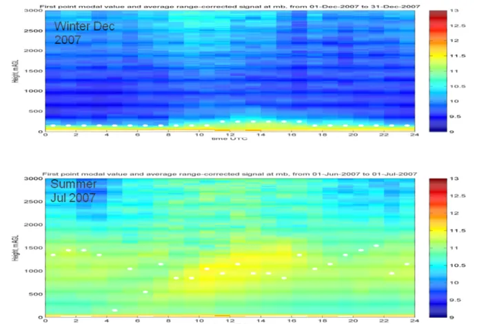
Figure 3: This is an example of LIDAR product for winter and summer, the white dot indicates the height of ML determined from the lidar signal , in the top, we have a characteristic winter PM distribution, where the stable atmospheric condition determines that the aerosol is confined in the first layers of atmosphere, in the bottom a indeed during the summer we note an increment of the mixing of the particulate matter in atmosphere (yellow color) and an increment of the PBLH until 1500 m ). During the night Residual High-level layers are visible in the lidar traces. These likely come from ‘old’ aerosol pumped up by convection on previous days and then trapped within stable layers, ( this is typical in third part of the day because the sedimentation is often slowly during the early morning until it reaches the new upwelling convective layer) This ‘residual’ layer may cause errors in the evaluation of the MH from lidar data
3.1 The importance of the mixing layer height - Meteorological Model estimate vs
Lidar estimate
The mixing layer height (MH) is an important parameter in air pollution modelling, the accurate simulation of evolution and structure of the Planetary Boundary Layer (PBL) has important implications for predicting and understanding the dynamics particulate matter (Zhang et al., 2006b; Miao et al., 2007), since it determines the effective volume in which pollutant are dispersed (Athanassiadis et al., 2002), and because PBL height is usually used in turbulent mixing parameterization (Troen and Mhart, 1986; Vautard et al., 2007 ). Substances emitted or originated near the surface are gradually dispersed horizontally and vertically through the action of turbulence, and finally become quasi-completely mixed throughout the PBL. The simulation of the time-resolved MLH is still critical in mesoscale models and in this context the comparison of model simulations with observed data is of particular importance to evaluate the performances of the model in a specific configuration. In order to evaluate the performances of the PBLH estimate by MM5 in MRF2, comparison with estimates obtained from observed data has been made in this work.
3.2 Comparison of mixed –layer evolution as inferred from lidar, balloon
observation and MM5 simulations in Milan –Bicocca (Italy)
Since the sun irradiance plays a key role in determining the PBL height the establishment of free convection, cloud free days (both modelled and observed) were chosen. Different episodes have been selected for the comparison. These correspond to typical clear sky summer and winter time conditions, in free convection regime.
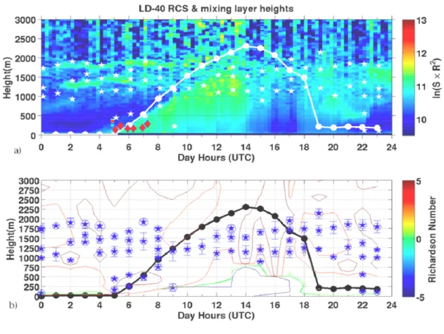
An example of the common results obtained with MRF2 MM5 PBL scheme are presented (fig. 4 and fig. 5)
Figura 4: Summer case of 13th July 2007. a) panel : a comparison among 1) hourly MH values estimated by MM5 with MRF2 parameterization (white line with filled circles), 2) MH derived from tethered balloon data (red diamonds) and 3) lidar Range-Corrected Signal (RCS) derivatives (white stars). b) panel: a comparison among hourly MH values estimated by MM5 with MRF2 parameterization (black line with filled circles), the MM5 Richardson Number (contour lines) and the lidar RCS derivative maxima ± standard deviation (blue asterisks, and error-bars) and magnitude of the derivatives (dimension of blue circles)
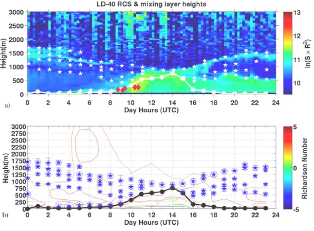
Figure 5: 11 February 2008: The same as fig 4 , but, for February 11, 2008
The upper panels in fig. 4 and fig 5 , show the contour plot of the lidar Range Corrected Signal, RCS. The automated retrieval from lidar data determines the MH as the lowest altitude of derivative (for each hour) of the RCS. Because of the low maximum altitude the tethered balloon can reach, OPC data are only available in the early morning, when the MH data are present, they are generally in good agreement with both the lidar-derived and the model MH determinations. The most important OPC-to-lidar discrepancies occur in the late OPC measurements, when the lidar MH exceeds 500m, and the OPC does not probably reach it. In figure 4 and fig 5, a high-level aerosol layer is evident during the night time. This has been found to be typical for Milan. This layer likely come from ‘old’ aerosol pumped up by convection on previous days. It is then trapped within stable layers. Sedimentation makes it often fall down slowly during the early morning until it reaches the new upwelling convective layer. The presence of this layer keeps the lidar-derived MH
higher than the modeled one both in the early morning and after the sunset in summer (fig 4) and in particularly after the sunset in winter (fig 5). This ‘residual’ layer may cause errors in the evaluation of the MH from lidar data. This is particularly true when the real height of the mixing layer is very low. In fact , due to technical reasons (overlap between the field of view and the emitted laser pulse ) the lidar cannot detect stratifications lower than about 60 m. Overall, the lidar-model comparison is most reliable from sunrise to sunset, when the aerosol is a particularly good marker to detect the MH (particulate matter from ground is uplifted by buoyancy, marking the PBL top). This process takes place mainly in clear sky and very low wind intensity conditions, so that the development of the mechanical turbulence doesn’t play a role. For this reason we selected days where free convection regime dominated on forced convection. Panels b, of Figure 4 and 5 show the MH as predicted by the MRF scheme (MM5, v3 r3-6) as well as the isoline of Rib. In this case, the MH is computed by using a thermodynamic approach, using a model described by throen and Mahrt able to determine the height of the mixing layer. This scheme is based only on stability conditions. In this case, the Richardson number does not determine directly the MH, since the ground temperature, the vertical wind speed as well as the virtual potential temperature profiles enter in its determination. For low wind speeds, the calculation becomes analogous to the Holzworth method (Holzworth, 1964). As predictable, the Rib isolines are then not correlated to the MH. While in the winter case the predicted MH is quite close to lidar-derived ones, in the summer case a noticeable overestimate is visible, evne assuming the highest aerosol stratification as the top of the convective layer. The problem could arise because the MRF approach, as said before, uses the prediction of the ground virtual potential temperature to infer the MH. The latter parameter, however, is then critical and rather hard to calculate, and may then bias the whole MH estimation. In the summer case it is also evident a cleaning of the lower atmosphere in the early afternoon. This is caused by breezes, deductible both from calculated and measured wind field.
3.3 Comparison Models vs Balloon data
In order to better understand how the model is able in reproducing the daily evolution and structure of the Planetary Boundary Layer , comparison between model temperature and humidity with balloon measurement has been made (Fig.8):
Figura 7
The fair weather ABL (Atmospheric Boundary Layer) consists of the componetns sketched in Fig 7. During day time there is a statically-unstable mixed layer (ML). At night, a statically stable
boundary layer (SBL) forms under a statically neutral residual layer (RL). The residual layer contains the pollutants and moisture from the previous mixed layer, but is not very turbolent. The bottom 20 to 200 m of the ABL is called the surface layer (fig 7) . Here frictional drag, heat conduction, and evaporation from the surface cause substantial changes of wind speed, temperature, and humidity with height. However, turbolent fluxes are relatively uniform with height; hence, the surface layer is known as the constant flux layer. Separating the free atmosphere from the mixed layer is a strongly stable entrainment zone (EZ) of intermitted turbolence. Mixed-layer depth is the distance between the ground and the middle of the EZ. At night, turbolence in the EZ cases, leaving a nonturbolent separation layer called the cappinginversion (CI), which is still strongly statically stable.
Figura 8) : Torre Sarca-Milano Bicocca -PROFILE T, RH and #/m3 ON JULY 14th at different hours a) 50 minutes after sunrise, b) 1
hour after sunrise c) 2 hour after sunrise d) 3,5 hours after sunrise , e) 4,5 hours after sunrise
Fig 8 shows an example of the comparison between model vertical results and balloon data collected during two intensive campaigns in summer 2007 and in winter 2008 in the frame of the
green line we have model results, fig.8a shows the profiles at the first lunch around 5- 5.35 Local Time, the mixed layer is confined at the first 100 m, stable layer is confined between 100 m- 300m and as for Stull framework upper this level is confined the residual layer.The model underestimate temperature and overestimates RH mainly in the upper level. Fig.8b shows the profiles at 5.40-6.18 and is interesting to notice a fast development of the mixing layer which in 30 minutes improve of 100 meters . Fig8c shows the third lunch at 6-7.15 , the humidity panel highlight that the model doesn’t capture the inversion at 300 m and overestimate this important variable, which plays a key role in heterogeneous chemistry. Fig8d shows the forth lunch at 7.40-8.27 therefore four hour after sunrise, at this time the residual layer is eroded and the mixing height reach 350 meters, in the last lunch, the fifth, fig8e 4,5-5 hour after sunrise we have a full and complete mixing and it seems that the model performs better when full mixing is reached, but still underestimates T. In conclusion Balloon-borne although observations are restricted to first few hours after sunrise and 700 m ca, however, they provide a very good description of the early morning development of the Mixing Layer, On 14th July a typical (“Stull”-like) PBL evolution is particularly clear: erosion of nocturnal and residual layers is completed after 2 and 4 hours after sunrise respectively, MM5 underestimates T profile, by 2-4 K and overestimates humidity above the nocturnal inversion, which is not well reproduced. When full mixing is reached after sunrise, model performs better and q is overestimated also after full mixing is reached by 2 g/kg
3.4 First Comparison CHIMERE model vs Lidar data
In Figure 9 we have an example of the comparisons done between PM vertical profile calculated from CHIMERE and the PM vertical profile detected by LIDAR.
The model shows a very good agreement with observation in time and in space, for example CHIMERE is able in reproducing the vertical PM plume, from the start of mixing of the particulate
matter due to the convection until his complete upwelling in the upper layers around 12 o’clock when the convection is more intense .
Figure 9
3.5 Case study
The preliminary results obtained comparing PM vertical profile calculated from CHIMERE and the PM vertical profile detected by LIDAR have suggested to use the model as instruments for interpretation of the observation in this area, so we focused our attention on seven days during summer 2007 from 12 to 18 July 2007, these correspond to typical clear sky and stable meteorological conditions, in free convection regime.
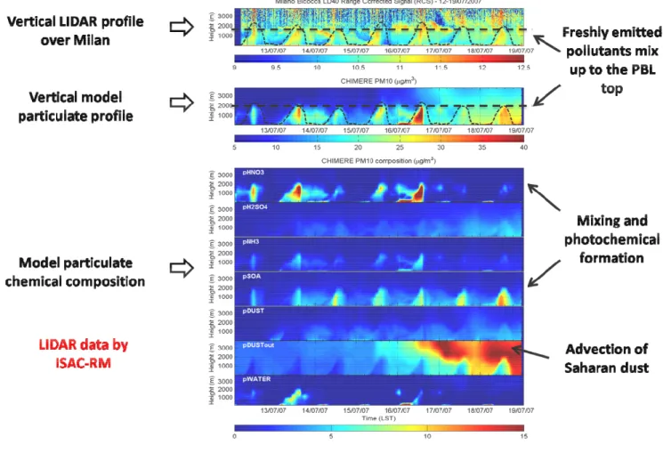
Figura 10: Seven days (12-17 July 2007) comparison between Vertical Lidar particulate profile and Vertical model particulate profile
Fig.10, show the results from the comparison between vertical lidar particulate profile and vertical model particulate profile. CHIMERE model in general reproduce well temporally and spatially the diurnal vertical distribution of the aerosol load detected by lidar. In the upper panel we can see the diurnal evolution of PM profile detected by lidar, which is normally characterized by the development of a plume during the morning and a clearing during the afternoon due to the mountain breeze , typically the plume reaches the top of the boundary layer which is located between 1500-2000 m around mid day and in this time we observed the highest concentrations in the upper levels. During the last two days we observes enhancement aerosols concentrations above the boundary layer which is probably due to Saharan dust intrusion. In comparison in Fig10, respectively, in the second image and in the follow ones we show the simulated pm10 profile and his some components as calculated by CHIMERE. We
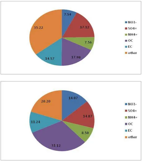
can note as the mode broadly reproduce the temporal end vertical features of the lidar signal, we have very good agreement concerning the development of the plume and clearing during afternoon. The model also predicts highest concentration in the upper levels of the PBL. It also reproduce the dust intrusion during the last two days and give an important information confirmed that this is due to the dust out intrusion as we can see from the DUST OUT panel obtained from CHIMERE simulation. Another important information from the model regard the composition , it predicts that a large part of the plume is composed by nitrate, in particular during 13 and 16 July 2007 , confirming the model tendency to overestimates the nitrous component in the particular matter, as we have observed also in the ground comparison measurements collected in Milano Bicocca (fig 11)
Figura 11: PM2.5 composition at the Milan station as measured (top) and modeled (bottom) in summer May-July 2007. Chimere overestimates the nitrous component and organic carbon with respect to measurements
This chapter will investigate the answers of CHIMERE model to the varying parameters in order to explain with a modelling approach the vertical profile observed in Milan area .
4.1 Sensitivity Test
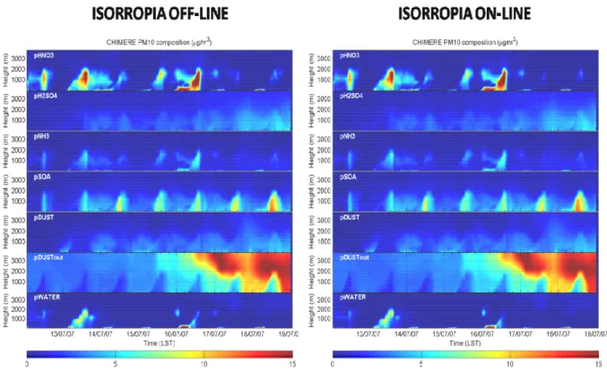
The thermodynamic equilibrium model ISORROPIA is used to determine the particle/gas partitioning of semi-volatil inorganic species. The model calculate the thermodynamical equilibrium of the system: sulfate-nitrate-ammonium-sodium-chloride-water at a given temperature and relative humidity. The solid/liquid phase transition is solved by ISORROPIA by computing the deliquescent relative humidities (transition relative humidity between the phases). In the CHIMERE model, the calculation of the thermodynamic equilibrium can be done by interpolating a look-up table .This look-up table has been pre-calculated, the partitioning coefficient for the nitrates and ammonium, and the aerosol water content has been calculated for range of temperature from 260 to 312K, for relative humidity from 0.3 to 0.99 and for concentrations from 10−2 to 65 µ.g.m−3.
Figura 12: ON-LINE VS OFF-LINE CALCULATION OF THERMODYNAMIC EQUILIBRIUM
The comparison shows the use of an on-line does not alter results (fig 12) , it leads only to a weak increase of the mean concentrations for the nitrates. As in the first sensitivity test we evaluate the impact of the Saharan dust on model results (fig.13). We made a run considering the dust out in the Boundary conditions and another one without the dust , as we can see inorganic and organic phases are insensitive to Saharan dust, indeed, model does not include parameterization of the nitrate-dust feedback. These last results allow to say that aerosol changes during Saharan dust event (17-18 July 2007) where we can note increment in pSOA concentrations (fig 13) are solely attributable to changes in meteorology. The third sensitivity test performed was on temperature variation (fig 14). We have increased temperature of 2 K, which is the magnitude of temperature model bias, CHIMERE, in this case seems to be more sensitive to this meteorological variable with a decrease of pHNO3 and weather in particular, but, this parameter doesn’t explain the nitrate increase in the upper level of the atmosphere during 12-16 July 2007, in this case temperature variation reduces nitrate concentration but does not change general conclusion. The greater concentration and
different humidity behavior during 13 and 16 July (fig 15) make humidity the number one candidate to explain why the large part of the plume in these two days is composed by nitrate, but remain the question, what for “Saharan days”? where we have as in 3 and 16 July high humidity level but low nitrate concentration.
In order to understand and explain the high nitrate concentration plume during 13 and 16 July we have performed other sensitivity tests, in particular we have decreased NOx (fig . 15) and NH3 (fig. 16) emissions for 40 % and decreased the humidity for 20% (fig.17).
As in the previous tests the model answer linked to the perturbation of these parameters is slight , Probably the parameter variation entity is too low, in particular what about the humidity, for to have a sensible chemical answer from the model.
The 20% reduction of the specific humidity, for example, lead to an important droop in the particulate matter water content but this not affect the composition of the plume in the upper level of the atmosphere, we observe (fig.17) only a very slight decrement of the nitrous component which suggest that the greater humidity levels during 13-16 July 2007 can’t explain alone the very high level concentration of NHO3 component in the aerosols in these days.
The last sensitivity test that we have performed was temperature decrement (fig 20) and diffusion reduction (fig 19) in order to understand why during similar meteorological and emission days as for example at 16 July and 18 July the plume composition present an important difference in nitrous content.
As we said the humidity in these days is very comparable (fig. 15), the principal difference we can note fig (15), are in temperature and in terms of the diffusion parameter.
The diffusion parameter reduction doesn’t determine a sensible variation of the content of nitrate in the plum simulated (fig. 19) indeed temperature reduction (fig.20) seems to be the most influential parameter which could be explain the difference between 13 and 16 July in chemical composition, even if it can’t the only causes of these differences.
In fact, figure 21 shows the importance of the absorption during the 13 July in the determination of so high nitrate levels in the upper level of the atmosphere. We set the absorption processes to zero for the 16 July, we can note (fig 21) how during 16 July this phenomena play an important role reducing the nitrous concentration of 8 ug/m3 so the model seem more sensitive on this parametrized physical process.
Figura 14: the sensitivity test for temperature
Figura 15: on the right : meteorological variables vertical profile , in order, from top panel to the bottom : temperature (t), specific humidity (sphu) , vertical wind component (winz), meridional wind component (windm) and diffusivity (Kz) -on the left : the simulated pm10 profile and his some components as calculated by CHIMERE
Figura 16 NH3 reduction test
Fig 18: Specific Humidity reduction test
Chapter 5
Conclusions
This work consists of a modeling analysis of the vertical structure of particulate matter and at a site near the city of Milan. This analysis was carried out comparing the model results with LiDAR continuous observations and balloon profiles collected during two intensive campaigns in summer 2007 in the frame of the ASI/QUITSAT project.
The model is able to reproduce with reasonable skill the observed aerosol vertical distribution from the start of mixing of the particulate matter due to the convection until its complete upwelling in the upper layers around midday when the boudary layer reaches its top. The model reproduced the dust intrusion and the structure of the residual layers detected by LiDAR. This last point provided interesting insights in the evaluation of the Mixing Height from LiDAR.
The modeling approach used here allowed gain of information about chemical composition of the aerosol plume. CHIMERE model predicts that a large part of the plume is composed by nitrate and secondary organic aerosol. During 13 and 16 July 2007 model predicts very high concentrations of nitrates which lead to unrealistically high PM concentration not detected by LIDAR. Moreover, the model has a general tendency to overestimates the nitrate component in the particular matter, as revealed by comparison with ground measurements collected at Milano Bicocca site.
Sensitivity studies show that there are a combination of different factor which determine the prevailing nitrate composition of the “plume”, in particular: humidity, temperature and gas absorption process.
Bibliografia
Athanassiadis, G. A., Rao, S.T., Ku, J.-Y., Clark, R.D., 2002. Boundary layer evolution and its influence on ground-level ozone concentrations, Environmental Fluid Mechanics 2, 339–357. Andreae, M. O., C. D. Jones, and P. M. Cox (2005), Strong present-dayaerosol cooling implies a hot future, Nature, 435, 1187–1190.
Andreani S., Keller J., Prévot S.H., Baltensperger U., Flemming J., 2008. Secondary aerosols in Switzerland and northern Italy: Modeling and sensitivity studies for summer 2003, Journal of Geophysical Research 113 (D06303), doi:10.1029/2007JD009053.
Angelino E., Bedogni M., Carnevale C., Finzi G., Minguzzi E., Peroni E., Pertot C., Pirovano G., Volta M, 2007. PM10 Chemical Modeling Simulation Over Northern Italy in the Framework of the CityDelta Exercise, Environ. Model Assess. 13:401-413
Aumont, B., F. Chervier, and S. Laval (2003), Contribution of HONO sources to the NOx/HOx/O3 chemistry in the polluted boundary layer, Atmos. Environ., 37, 487. 498
Baertsch-Ritter, N., Prevot, A. S. H., Dommen, J., Andreani-Aksoyoglu, S., Keller, J., 2003. Model study with UAM-V in the Milan area (I) during PIPAPO: simulation with changed emissions compared to ground and airborne measurements, Atmospheric Environment 37, 4133-4147.
Bessagnet, B., Hodzic, A., Vautard, R., Beekmann, M., Rouil, L., Rosset, R., 2004. Aerosol modeling with CHIMERE first evaluation at continental scale. Atmospheric Environment 38, 2803– 2817
Bessagneta B. , Hodzicb, A., Blancharda, o., Lattuatic, M., Le Bihana, O. , Marfaingc, H., Rouıl L., Origin of particulate matter pollution episodes in wintertime over the Paris Basin. Atmospheric Environment 39 6159-6174
Chen F., Dudhia, J., 2001a. Coupling an advanced land surface-hydrology model with the Penn State-NCAR MM5 modeling system: Part I – model implementation and sensitivity. Mon Wea Rev 129, 587-604
Derognat, C., Beekmann, M., Ba umle, Martin, D., 2003. Effect of biogenic volatile organic compound emissions on tropospheric chemistry duringthe atmospheric pollution over the Paris area (ESQUIF) campaign in the Ile-de-France region. Journal of Geophysics Research 108 (D14), 4409– 4423
Gelbard, F., and J. H. Seinfeld (1980), Simulation of multicomponent aerosol dynamics, J. Colloid Interface Sci., 78, 485. 501
G. Grell, S. Dudhia, D. R. Stauffer, 1994. A description of the fifth generation of Penn. State/NCAR mesoscale model (MM5). NCAR/TN-398+STR, Natl.Cent. For Atmos. Res., Boulder, Colo.
Guelle,W., Y. J. Balkanski, J. E. Dibb, M. Schulz, and F. Dulac (1998), Wet deposition in a global size-dependent aerosol transport model: 2. Influence of the scavenging scheme on 210Pb vertical profiles, surface concentrations, and deposition, J. Geophys. Res., 103, 28,875.28,891
Hong, S. H., Pan, H. L., 1996. Nonlocal boundary layer vertical diffusion in a medium-range forecast model, Monthly Weather Review 124, 2322-2339.
Jacob, D. J. (2000), Heterogeneous chemistry and tropospheric ozone, Atmos. Environ., 34, 2131. 2159
Kulmala, M., A. Laaksonen, and L. Pirjola (1998), Parameterization for sulfuric acid/water nucleation rates, J. Geophys. Res., 103, 8301. 8307.
Liu, Y., Park, R. J., Jacob, D. J., Li, Q., Kilaru, V., and Sarnat, J. A.: Mapping annual mean ground-level PM2.5 concentrations using multiangle imaging spectroradiometer aerosol optical thickness over the contiguous united states, J. Geophys. Res., 109, D22206, doi:10.1029/2004jd005025, 2004. Martilli, A., Neftel, A., Favaro, A., Kirchner, F., Sillman., S., Clappier, A., 2002. Simulation of the ozone formation in the northern part of the Po Valley, Journal of Geophysical Research 107(D22), 8195, doi:10.1029/2001JD000534.
Miao, J.-F., Chen, D., Wyser, D., Borne, K., Lindgren, M. K. S., Strandevall, J., Thorsson, S., Achberger, C., Almkvist, E., 2008. Evaluation of MM5 mesoscale model at local scale for air quality applications over Swedish west coast: Influence of PBL and LSM parameterizations, Meteorology and Atmospheric Physics 99, 77-103.
Mlawer, E.J., Taubman, S.J., Brown, PD., Iacono, M.J., Clough, S.A., 1997. Radiative Transfer for inhomogeneous atmospheres: RRTM, avalidated correlated-k model for the longwave. Journal of Geophysical Research 102 (D14), 16663-16682
Nenes, A., Pilinis, C., Pandis, S.N., 1999. Continued development and testing of a new thermodynamic aerosolmodule e for urban and regional air quality models. Atmospheric Environment 33, 1553–1560.
Nenes, A., C. Pilinis, and S. N. Pandis (1998), ISORROPIA: A new thermodynamic model for inorganic multicomponent atmospheric aerosols, Aquat. Geochem., 4, 123. 152.
Nenes, A., S. N. Pandis, and C. Pilinis (1999), Continued development and testing of a new thermodynamic aerosol module for urban and regional air quality models, Atmos. Environ., 33, 1553. 1560.
Pankow, J. F. (1994), An absorption model of gas/particle partitioning of organic compounds in the atmosphere, Atmos. Environ., 28, 185. 188.
Penner, J. E., et al. (2002), A comparison of model- and satellite-derived aerosol optical depth and reflectivity, J. Atmos. Sci., 59, 441– 460
Petters, M. D., A. J. Prenni, S. M. Kreidenweis, P. J. DeMott, A. Matsunaga, Y. B. Lim, and P. J. Ziemann (2006d), Chemical aging and the hydrophobic- to-hydrophilic conversion of carbonaceous aerosol, Geophys. Res. Lett., 33(24), L24806, doi:10.1029/2006GL027249
Roberts, S. , 2003 Combining data from multiple monitors in air pollution mortality time series studies. Atmospheric Environment 37, 3317-3322
Reisner, J., Rasmussen, R.M., Bruintjes, R.T., 1998. Explicit forecasting of supercooled liquid water in winter storms using the MM5 mesoscale model. Quarterly Journal of the Royal Meteorological Society 124B, 1071-1107
Rita Van Dingenen, Frank Raes, Jean-P. Putaud, Urs Baltensperger, Aure!lie Charron, M.-Cristina Facchini, Stefano Decesari, Sandro Fuzzi, Robert Gehrig, Hans-C. Hansson, Roy M. Harrison,
Cristoph Hu.glin, Alan M. Jones, Paolo Laj, Gundi Lorbeer, Willy Maenhaut, Finn Palmgren, Xavier Querol, Sergio Rodriguez, Ju.rgen Schneider, Harry ten Brink, Peter Tunved, Kjetil Trseth, Birgit Wehner, Ernest Weingartner, Alfred Wiedensohler, Peter Wahlin (2004), A European aerosol phenomenology—1: physical characteristics of particulate matter at kerbside, urban, rural and background sites in Europe, Atmospheric Environment 38 , 2561–2577
Rosenfeld, D., Lohmann, U., Raga, G.B., O'Dowd, C.D., Kulmala, M., Fuzzi, S., Reissell, A., AndreaeM.O. 2008. Flood or Drought: How Do Aerosols Affect Precipitation? Science Vol. 321. no. 5894, (1309 – 1313) DOI: 10.1126/science.1160606
Schmidt, H., Derognat, C., Vautard, R., Beekmann, M., 2001. A comparison of simulated and observed ozone mixing ratios for the summer of 1998 in western Europe. Atmospheric Environment 35, 6277–6297.
Seinfeld, J. H., and S. N. Pandis (1998), Atmospheric Chemistry and Physics, John Wiley, Hoboken, N. J.
Seigneur, C. Current Status of air quality models for particulate matter, J. Air Waste Manage. Assoc., 51 (11), 1508-1521, 2001.
Silibello C., Calori G., Brusasca G., Giudici A., Angelino E., Fossati G., Peroni E., Buganza E. 2008. Modelling of PM10 concentrations over Milano urban area using two aerosol modules, Enviromental Modelling & Software., 23 333-343
Vautard, R., Maidi, M., Menut, L., Beekmann, M., Colette, A., 2007. Boundary layer photochemistry simulated with a two-stream convection scheme, Atmospheric Enviroment 41, 8275-8287.
Vautard, R., Martin, D., Beekmann, M., Drobinski, P., Friedrich, R., Jaubertie, A., Kley, D., Lattuati, M., Moral, P., Neininger, B., Theloke, J., 2003. Paris emission inventory diagnostics from
ESQUIF airborne measurements and a chemistry transport model. Journal of Geophysics Research 108 (D17), 8564–8585.
World Health Organization, 2005 Air quality guidelines for Europe. WHO Regional Publications, European Series, No. 91
Zhang, J. and Rao, S.T., 1999. The role of vertical mixing in the temporal evolution of ground level ozone concentrations, Journal Applied Meteorology 38, 1674-1691.
Zhang, K., Mao, H., Civerolo, K., Berman, S., Ku, J., Trivikrama Rao, S., Doddridge, B., Russel, B., Philbrick and Richard Clark, 2001. Numerical investigation of boundary-layer evolution and nocturnal low level jets: Local versus non local PBL schemes, Enviromental Fluid Mechanics 1, 171-208.
Zhang, Y., Pun, B., Vijayaraghavan, K., Wu, S. Y., Seigneur, C., Pandis, S. N., Jacobson, M. Z., Nenes, A., and Seinfeld, J. H.: Development and application of the model of aerosol dynamics, reaction, ionization, and dissolution (MADRID), J.Geophys. Res., 109 (D1), D01202, doi:10.1029/2003JD003501, 2004.
Zhang, Y., Liu, P., Pun, B., Seigneu, C., 2006a. A comprehensive performance evaluation of MM5-CMAQ for the Summer 1999 Southern Oxidants Study episode - Part I: Evaluation protocols, databases, and meteorological predictions, Atmospheric Environment 40, 4825-4838.
Zhang, Y., Liu, P., Queen, A., Misenis, C., Pun, B., Seigneur, C., Yuh, S. W., 2006b. A comprehensive performance evaluation of MM5-CMAQ for the Summer 1999 Southern Oxidants Study episode - Part II: Gas and aerosol predictions, Atmospheric Environment , 40, 4839-4855.
.
. .