Computational Intelligence for classification and forecasting of solar photovoltaic energy production and energy consumption in buildings

Eleonora D’Andrea

Computational Intelligence for

classification and forecasting of solar

photovoltaic energy production and

energy consumption in buildings

Anno 2013

UNIVERSITÀ DI PISA

Scuola di Dottorato in Ingegneria Leonardo da Vinci

Corso di Dottorato di Ricerca in

Ingegneria dell Informazione

UNIVERSITÀ DI PISA

Scuola di Dottorato in Ingegneria “Leonardo da Vinci”

Corso di Dottorato di Ricerca in

Ingegneria dell’Informazione

Tesi di Dottorato di Ricerca

Computational Intelligence for

classification and forecasting of solar

photovoltaic energy production and

energy consumption in buildings

Autore:

Eleonora D’Andrea _________________

Relatori:

Prof. Beatrice Lazzerini _______________ Prof. Francesco Marcelloni _______________ Ing. Marco Cococcioni ________________

Anno 2013 SSD ING-INF/05

“Non sono le specie più forti quelle che sopravvivono e nemmeno le più intelligenti, ma quelle in grado di rispondere meglio al cambiamento”

“It is not the strongest of the species that survive, nor the most intelligent, but the one most responsive to change” [Charles Darwin]

Sommario

Questa tesi presenta una serie di nuove applicazioni di tecniche di Computational Intelligence in problemi del settore energetico, con particolare riferimento alla valutazione dell'energia prodotta da impianti fotovoltaici e alla valutazione dei consumi energetici di edifici. Infatti, di recente, grazie anche alla crescente evoluzione tecnologica, il settore energetico ha attirato l'attenzione della comunità di ricerca scientifica nel proporre strumenti utili in problemi di efficienza energetica negli edifici e nella gestione della produzione di energia solare. Affronteremo quindi due tipologie di problemi.

Il primo problema è legato alla gestione efficiente degli impianti solari fotovoltaici, per esempio, per controllare efficacemente le prestazioni e per la ricerca di guasti, o per la pianificazione della distribuzione di energia elettrica in rete. Questo problema è stato affrontato con due approcci diversi: un approccio di previsione e un approccio di classificazione fuzzy per stimare la produzione di energia, a partire dalla conoscenza di alcune variabili ambientali. Il sistema di previsione sviluppato è in grado di riprodurre la curva giornaliera di energia prodotta dai pannelli solari dell'impianto, con un orizzonte temporale di previsione di un giorno. Il sistema sfrutta reti neurali e modelli di analisi di serie temporali. Il sistema di classificazione fuzzy, invece, estrae una certa conoscenza linguistica relativa alla quantità di energia prodotta dall'impianto, sfruttando una base di regole fuzzy ottimale e impiegando algoritmi genetici. Il modello sviluppato è il risultato di una nuova metodologia di tipo gerarchico per la costruzione di sistemi fuzzy, che può essere applicata in molteplici settori.

Il secondo problema è legato alla efficienza energetica degli edifici, allo scopo di ottenere benefici quali la riduzione del costo o la pianificazione del carico, ed è stato affrontato proponendo un sistema di previsione dei consumi energetici negli uffici. Il sistema sviluppato sfrutta una rete neurale per stimare il consumo di energia per illuminazione in un intervallo di tempo di alcune ore, a partire da considerazioni sulla luce naturale esterna disponibile.

Abstract

This thesis presents a few novel applications of Computational Intelligence techniques in the field of energy-related problems. More in detail, we refer to the assessment of the energy produced by a solar photovoltaic installation and to the evaluation of building’s energy consumptions. In fact, recently, thanks also to the growing evolution of technologies, the energy sector has drawn the attention of the research community in proposing useful tools to deal with issues of energy efficiency in buildings and with solar energy production management. Thus, we will address two kinds of problem.

The first problem is related to the efficient management of solar photovoltaic energy installations, e.g., for efficiently monitoring the performance as well as for finding faults, or for planning the energy distribution in the electrical grid. This problem was faced with two different approaches: a forecasting approach and a fuzzy classification approach for energy production estimation, starting from some knowledge about environmental variables. The forecasting system developed is able to reproduce the instantaneous curve of daily energy produced by the solar panels of the installation, with a forecasting horizon of one day. It combines neural networks and time series analysis models. The fuzzy classification system, rather, extracts some linguistic knowledge about the amount of energy produced by the installation, exploiting an optimal fuzzy rule base and genetic algorithms. The developed model is the result of a novel hierarchical methodology for building fuzzy systems, which may be applied in several areas.

The second problem is related to energy efficiency in buildings, for cost reduction and load scheduling purposes, and was tackled by proposing a forecasting system of energy consumption in office buildings. The proposed system exploits a neural network to estimate the energy consumption due to lighting on a time interval of a few hours, starting from considerations on available natural daylight.

Table of Contents

SOMMARIO

ABSTRACT

TABLE OF CONTENTS

LIST OF ACRONYMS AND ABBREVIATIONS

LIST OF FIGURES

LIST OF TABLES

INTRODUCTION

1

ARTIFICIAL NEURAL NETWORKS

1.1 Introduction 3

1.2 The biological neuron 3

1.3 An overview of neural networks 4

1.3.1 The perceptron 5

1.4 The multilayer perceptron neural network 6 1.4.1 The backpropagation training algorithm 7 1.5 Neural networks for time series forecasting 8 1.5.1 The NARX neural network 10

2

FUZZY SYSTEMS

13

2.1 Introduction 13

2.2 Overview of Fuzzy Rule-Based Classifiers 14 2.3 The implementation of a FRBC: frbc 15 2.3.1 The rule base construction 16 2.3.2 The fuzzy reasoning method 18

3

GENETIC ALGORITHMS AND HYBRID SYSTEMS

21

3.1 Introduction 21

3.2 Genetic algorithms: main concepts 21

3.2.1 GA operators 22

4

ONE DAY-AHEAD FORECASTING OF PV ENERGY PRODUCTION BY

25

4.1 Introduction 25

4.1.1 Outline of the chapter 27 4.2 Description of the solar PV dataset 27 4.3 The proposed NARX-neural network model for solar PV energy

forecasting 28

4.3.1 Choice of the structural and configuration parameters 29

4.3.2 Model refinement 31

4.4 Experimental results 33

4.4.1 Prediction of the instantaneous energy 34 4.4.2 Prediction of the accumulated energy 36

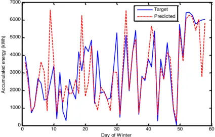
4.4.3 Discussion 41

4.5 Concluding remarks 42

5

A HIERARCHICAL APPROACH TO MULTI-CLASS FUZZY CLASSIFIERS

FOR PV ENERGY PRODUCTION

43

5.1 Introduction 43

5.1.1 Context of application 45 5.1.2 Outline of the chapter 46 5.2 Description of the real-world experimental dataset 46 5.3 A hierarchical approach to fuzzy classifier construction 47 5.3.1 First step: first-level grid partitioning 48 5.3.2 Second (iterative) step: deeper-level grid partitioning 49 5.3.3 Third step: final fuzzy model generation 50 5.3.4 GA-based parameter optimization 51 5.4 Application of the proposed methodology to the real-world dataset 52

5.4.1 First step 52

5.4.2 Second step 53

5.4.3 Third step 56

5.4.4 Genetic optimization 59 5.5 Experimental results on the PV dataset 60 5.6 Validation on benchmark datasets and discussion 61

5.6.2 Wisconsin breast cancer dataset 63 5.6.3 Pima Indians diabetes dataset 64

5.6.4 Wine dataset 65

5.7 Concluding remarks 66

6

NEURAL NETWORK-BASED FORECASTING OF ENERGY

CONSUMPTION DUE TO LIGHTING IN OFFICE BUILDINGS

67

6.1 Introduction 67

6.1.1. Outline of the chapter 69 6.2 Description of the building consumption dataset 69

6.3 The proposed model 70

6.3.1 Effects of climatic contest: analysis of solar irradiation 71 6.3.2 Analysis of energy consumption based on the office use 75

6.3.3 Discussion 76

6.4 Experimental results 77

6.5 Concluding remarks 79

7

THESIS CONCLUSION AND FUTURE WORK

81

ACKNOWLEDGEMENTS

83

REFERENCES

85

A

HOW TO IMPLEMENT A GENERIC CLASSIFIER IN PRTOOLS

95

A.1 PRTools framework 95

A.2 Basic elements of PRTools 96 A.2.1 The dataset object 96 A.2.2 The mapping object 97 A.3 The construction of a generic trained classifier xc 98 A.3.1 The classifier constructor xc 98 A.3.2 The training phase xc_train 98 A.3.3 The mapping phase xc_map 98 A.4 The implementation of frbc in PRTools 99 A.4.1 frbc (the constructor) 99

A.4.2 frbc_train (the training function) 100

A.4.3 frbc_map (the mapping function) 101 A.4.4 frbc: some usage examples 101

List of Acronyms and Abbreviations

Acronym Meaning

AC Alternating Current ANN Artificial Neural Network APE Absolute Percentage Error AR Auto-Regressive

ARIMA Auto-Regressive Integrated Moving Average CI Computational Intelligence

CF Certainty Factor

DB Data Base

DC Direct Current

DP Dominance Percentage

ECL Energy Consumption due to Lighting EP Electric Power

EU European Union FLT Fuzzy Logic Toolbox FRBC Fuzzy Rule-Based Classifier FRM Fuzzy Reasoning Method FS Fuzzy System

GA Genetic Algorithm GFS Genetic-fuzzy system

HFRBC-GA GA-optimized Hierarchical approach to Fuzzy Rule-Based Classifiers

HVAC Heating, Ventilation and Air Conditioning KB Knowledge Base

MAPE Mean Absolute Percentage Error MCF Multiple Certainty Factor MLP Multi-Layer Perceptron MSE Mean Squared Error

NARX Non-linear Auto-Regressive with eXogenous input PRTools Pattern Recognition Tools

PV Photovoltaic

R Coefficient of determination in Regression RB Rule Base

RMSE Root Mean Squared Error RT Relevance Threshold SCF Single Certainty Factor

List of Figures

Figure 1.1. A simplified model of the biological neuron. 4

Figure 1.2. The scheme of the perceptron. 5

Figure 1.3. The scheme of a MLP neural network having two inputs,

two outputs and one hidden layer with four neurons. 7

Figure 1.4. NARX model block diagram in closed loop mode. 9

Figure 1.5. The scheme of a simple NARX neural network (the figure

was produced in the Matlab® environment). 11

Figure 2.1. A fuzzy rule-based classifier. 14

Figure 2.2. An example of a fuzzy partition for the input variables, built

according to the Wang and Mendel approach. 17

Figure 3.1. The functioning of a simple GA in pseudocode. 22

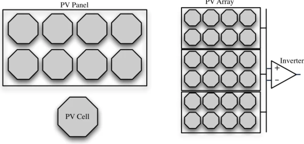
Figure 4.1. Photovoltaic elements: PV cell, PV panel, and PV array. 26

Figure 4.2. Solar irradiation trend for six days of Winter. 28

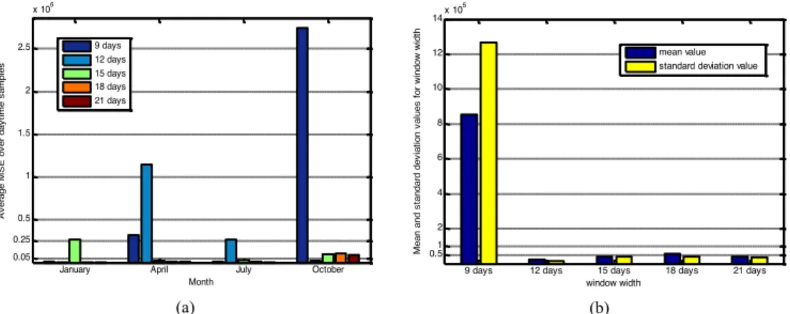
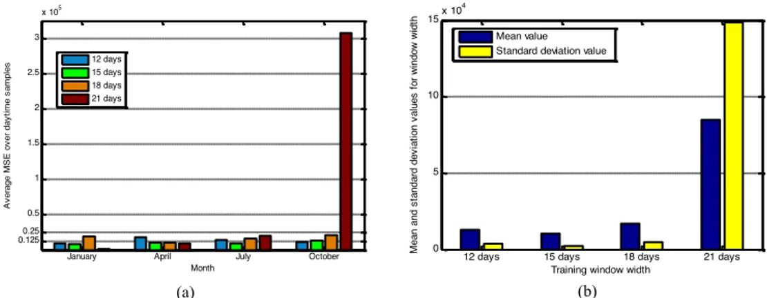
Figure 4.3. Forecasting performances obtained using irradiance only over

the daytime samples for whole months (January, April, July and October). (a) Average MSE. (b) Mean and standard

deviation of the average MSEs for each window width. 30

Figure 4.4. Forecasting scheme adopted. 31

Figure 4.5. NARX neural network model employed in the experiments

(the figure was produced in the Matlab® _{environment). 32}

Figure 4.6. Forecasting performances obtained using irradiance and hour

inputs over the daytime samples for the months of January, April, July and October. (a) Average MSE. (b) Mean and

standard deviation of the average MSEs for each window width. 32

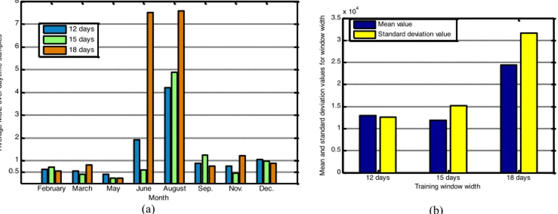
Figure 4.7. Forecasting performances obtained using irradiance and hour

inputs over the daytime samples for the months of February, March, May, June, August, September, November, and

December. (a) Average MSEs. (b) Mean and standard deviation of the average MSEs for each window width. 33

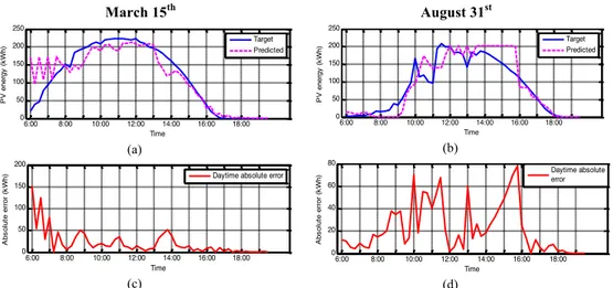
Figure. 4.8. Results on four well performing days chosen at random.

(a) (b) (e) (f) Comparison between the real energy and the predicted energy. (c) (d) (g) (h) Associated daytime absolute

instantaneous error. 35

Figure 4.9. Results on two atypical days chosen at random.

(a) (b) Comparison between the real energy and the predicted

Figure 4.10. Results on two unpredictable days chosen at random.

(a) (b) Comparison between the real energy and the predicted

energy. (c) (d) Associated daytime absolute instantaneous error. 36

Figure 4.11. Target and predicted daily accumulated produced energy for

Spring. 38

Figure 4.12. Target and predicted daily accumulated produced energy for

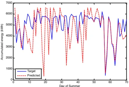
Summer. 38

Figure 4.13. Target and predicted daily accumulated produced energy for

Autumn. 39

Figure 4.14. Target and predicted daily accumulated produced energy for

Winter. 39

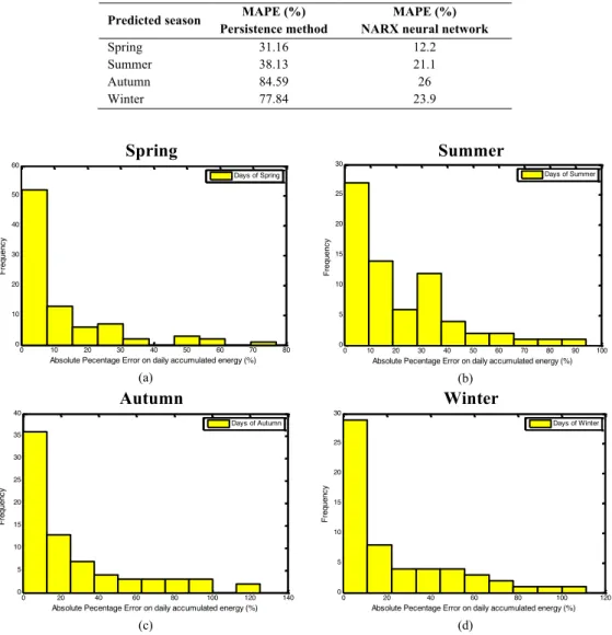
Figure 4.15. Error histograms for (a) Spring, (b) Summer, (c) Autumn,

and (d) Winter. 40

Figure 4.16. Error histogram for the best days of Spring (daily error lower

than 10%). 41

Figure 5.1. Scatter diagram of the PV dataset and distribution of the samples

over the three output classes (Low, Medium, High). 47

Figure 5.2. A to-subgrid area containing five univocal mapping areas

(colored areas), and the (hyper)rectangle (dashed line) including all the samples inside the univocal mapping areas. 50

Figure 5.3. Steps of the proposed hierarchical methodology and resulting

objects. 51

Figure 5.4. Partition of the input domain by applying the k-means clustering

algorithm (with k=3) and identification of 9 areas (numbered

from 1 to 9) on the grid. 52

Figure 5.5. Scaling from a uniform partition (a) to a non-uniform one (b). In

both cases, two-sided Gaussian membership functions are used. 53

Figure 5.6. Distribution of samples on the areas of the first-level grid:

(a) total, and (b) per class (logaritmic scale on y-axis). 54

Figure 5.7. The grid partitions of the original input space obtained by

applying the first step and the first iteration of the second step of the methodology (the dot notation is used to indicate sub-areas). 55

Figure 5.8. The grid partition of area 9.4 obtained through the second and

third iterations of the second step of the methodology. 55

Figure 5.9. Hierarchical decomposition tree. 57

Figure 5.10. Part of the final rulebase (compact notation). 58

Figure 5.11. Fuzzy sets built by the hierarchical method to model areas 1,

4, 9, and 9.4. 59

Figure 6.1. Statistics about energy consumption. (a) Total European energy

consumption. (b) Office buildings electric consumption. 67

Figure 6.2. Evolution of consumption (red dotted line) and irradiation (blue

solid line) from Monday May 9th _{to Sunday May 15}th_{. 70}

Figure 6.3. Solar irradiation and electrical consumption for four days of

June with different sky conditions: (a) two cloudy sky days, and

(b) two clear sky days. 71

Figure 6.4. Solar irradiation curves for four consecutive days of April. 72

Figure 6.5. Daily irradiation curves and corresponding typical ideal irradiation curve (black line) for (a) May, (b) June and

(c) September. 73

Figure 6.6. Typical ideal irradiation curves for six months (April to

September). 74

Figure 6.7. (a) Typical ideal irradiation curve (magenta dotted line) and actual irradiation curve (blue solid line) for four days of

September. (b) Difference between the two irradiation curves. 74

Figure 6.8. Evolution of the energy consumption for a typical working day.

Please note that, for the considered day, the working time ends

at 8 p.m.. 75

Figure 6.9. Identification of the time intervals over the working time. 76

Figure 6.10. Temporal evolution of the energy consumption for two

consecutive weeks of April. 76

Figure A.1. Flowchart describing the actions of the frbc constructor. 100

Figure A.2. Flowchart describing the actions of the mapping function

frbc_map. 101

Figure A.3. Decision boundaries for knnc, ldc and frbc (dashed red

List of Tables

Table 1.1. Some common activation functions. 7

Table 2.1. Mathematical equations for the aggregation functions. 20

Table 4.1. Parameters for the final NARX neural network model. 33

Table 4.2. Comparison between real and predicted accumulated energy. 37

Table 4.3. Comparison between the persistence method and the NARX

neural network. 40

Table 5.1. Application of the multi-class fuzzy classifier on the PV

dataset for 56 different FRMs (best results in bold). 60

Table 5.2. Final parameters of the merged fuzzy model for the

classification of solar energy production. 61

Table 5.3. Classification results on Iris dataset (best result in bold). 62

Table 5.4. Values of the GA-optimized model parameters for the

benchmark datasets. 63

Table 5.5. Classification results on Wisconsin cancer dataset (best result

in bold). 64

Table 5.6. Classification results on Pima Indians diabetes dataset (best

result in bold). 65

Table 5.7. Classification results on Wine dataset (best result in bold). 65

Table 6.1. Characteristics of the building. 69

Table 6.2. Inputs and output variables of the neural network. 77

Table 6.3. Learning parameters for the final neural network. 78

Introduction

In this thesis Computational Intelligence (CI) techniques are employed in applications regarding energy systems. Many papers exist concerning applications of CI to perform forecasting, classification, and pattern recognition in the energy field (e.g., heating, ventilation and air-conditioning (HVAC) systems, power-generation, load forecasting, building’s energy consumption, wind speed forecasting, solar irradiation estimation, etc.)

Computational intelligence includes several techniques, e.g., artificial neural networks, genetic algorithms, expert systems, and fuzzy systems. Each kind of technique allows building systems suited to solve a certain class of problem. Moreover, various hybrid systems may be created, as combinations of two or more of the systems previously mentioned, to exploit the advantages of both the techniques simultaneously. In addition, a brief description of forecasting through time series analysis is presented.

The thesis is organized as follows. Chapters 1 through 3 provide an overview of the computational intelligence techniques adopted in this thesis. In particular, Chapter 1 recalls main theory concepts about neural networks, describes the classical multi-layer perceptron neural network and the non-linear auto-regressive with exogenous input neural network model (NARX). In addition, some notions about forecasting and time series analysis are briefly recalled. Chapter 2 regards fuzzy rule-base classification systems. Particularly, the fuzzy rule-based classifier

frbc is presented, along with the fuzzy reasoning method and the methodology for automatic generation of rules from data, that frbc adopts. Finally, Chapter 3 provides an overview about genetic algorithms and a brief description of genetic-fuzzy hybrid systems. Chapters 4 through 6 contain the novelty of the thesis, i.e., the developed methodologies and the experimental results achieved. Two main problems are addressed. First, the management of energy production in solar photovoltaic (PV) installations, by classification and forecasting, and, second, the forecasting of energy consumption in buildings.

The interest for the first problem arises from the necessity of forecasting and/or classification tools for the analysis of energy production in solar PV installations. In fact, solar energy is becoming a valid alternative to traditional energy and, as a consequence, PV installations have spread in recent years. In addition, the monitoring of the performance of solar panels has become a key issue for the improvement of the efficiency of the PV installation, as well as for finding faults or for efficiently planning the energy distribution. Among other things, PV-based power generators are discontinuous energy sources, owing to the influence of weather conditions. For all these reasons, a set of management tools is needed to correctly exploit the PV installation productivity.

The problem is tackled from two different points of view. On the one hand, we propose a general methodology to forecast solar energy production with a

forecasting horizon of one day. The forecasting system, presented in Chapter 4, consists of a NARX time series analysis model implemented using a feed-forward neural network with tapped delay lines. The system, starting from some knowledge about solar irradiation, is able to faithly reproduce the instantaneous curve of daily produced energy, as well as to estimate the total daily produced energy. From another point of view, a further issue in PV energy production management is the lack of a fuzzy approach to data classification to make the final user able to make decisions easily regarding energy production management. In this way, even the non-expert user of PV systems might be able to understand the results and make smarter decisions, as we deal with class labels. Regarding this issue, we developed in Chapter 5 a fuzzy rule-based classification system aimed to classify the energy produced by a PV panel based on two environmental variables, i.e., the irradiation and the temperature of the panel. At the same time, we propose a novel hierarchical method to construct fuzzy classifiers, by performing an input domain space analysis with the aim of generating an optimal fuzzy rule base avoiding the generation of too many, unnecessary rules. The developed model results from the merging of a number of fuzzy systems built on input domain regions increasingly smaller. Each fuzzy system is developed exploiting the fuzzy rule-based classifier

frbc. The model is actually a genetic-fuzzy system, as the model parameters are optimized by a real-coded genetic algorithm.

The motivation for dealing with the second problem, i.e., the forecasting of energy consumption in buildings, stems from considerations about the large amount of energy consumed in buildings, also in reference to the political campaigns concerning energy efficiency and energy savings promoted by several countries. The chance of knowing building’s energy consumption in real time or even in advance could bring several benefits, such as cost reduction, energy management and control, and load scheduling in the electrical grid. Chapter 6 is devoted to address this problem. In particular, we refer to the electric lighting energy consumption in offices. The reason is that it is well known that electric lighting energy consumption is a big component of office buildings energy consumption. The proposed method uses an artificial neural network to forecast the average energy consumption on a time interval of a few hours, exploiting mainly the information about natural daylight, in terms of solar irradiation. The novelty of the proposed method stands mainly in the design of the forecasting system, which does not need any kind of information about the building to estimate its consumption.

Finally, Chapter 7 provides the thesis conclusions and future work, and Appendix A reports a guideline on how to implement a generic classifier (such as frbc) in the PRTools framework.

The research presented in this thesis was developed entirely using the toolboxes existing in the Matlab® environment. Additionally, the PRTools toolbox was used for pattern recognition concerns.

1

Artificial neural networks

1.1 Introduction

Artificial Neural Networks (ANNs) are data-driven intelligent systems having the capability to learn, remember and generalize. They were created to reproduce the learning process of the human brain by learning the relationship between input parameters and output variables based on previously recorded data [13, 98].

The human brain is a complex calculator, non-linear, massively parallel with abilities like learning, generalization and adaptability. Moreover it is fault tolerant. It is constituted by an extremely large number of simple processing elements (biological neurons) with many interconnections, thus being able to perform complex computations.

Thus, artificial neural networks have been developed following the structure and the functioning of biological neurons in the human nervous system.

Neural networks are widely applied in areas such as prediction, classification, recognition and control. Applications of artificial neural networks are in many fields: pattern classification, clustering, function approximation, prediction, optimization, and control.

In this chapter, a brief introduction to artificial neural networks is presented in Sections 1.2 and 1.3. Then, in Section 1.4 we address the multilayer perceptron neural network and the backpropagation training algorithm. Next, in Section 1.5, we present a description of main concepts about time series forecasting and finally we present a neural network model suited for forecasting purposes.

1.2 The biological neuron

A neuron is a special biological cell that processes information. It is composed of i) a cell body called soma, ii) many branched extensions called dendrites, through which the neuron receives electricity signals from other neurons, and iii) a filamentous extension, called axon, through which the electrical signals are transmitted to other neurons. The point of connection between two neurons (the terminal of the axon of one neuron and the dendrite of another one) is called

synapse. A simplified model of the biological neuron is depicted in Fig. 1.1.

dendrites and transmits signals generated by its cell body along the axon. We may refer to the dendrites as the inputs of the neuron, while to the axon as the output of the neuron.

Figure 1.1. – A simplified model of the biological neuron.

A neuron is activated by electric impulses coming from other neurons when an electric potential difference between the inside and the outside of the cell occurs. Then, if the sum of received inputs exceeds a certain threshold, the neuron fires an electrical impulse along its axon. This electrical impulse causes the release of certain chemicals, called neurotransmitters, from the terminals of the axon, which in turn may influence other neurons. The neurotransmitters diffuse across the synaptic gap, to enhance or inhibit (depending on the type of the synapse) the tendency of the receptor neuron to fire electrical impulses.

Further, the brain is able to adjust the connections between the neurons based on its experience, that is, it is able to learn.

In the brain, the various areas cooperate, influencing each other and contributing to the achievement of a specific task, without the need for a centralized control. In addition, the brain is fault tolerant, that is, if a neuron or one of its connections is damaged, the brain continues to function, although with slightly degraded performance.

1.3 An overview of neural networks

As already stated, an ANN is a collection of simple processing units individually interconnected. In its basic computational form, a neuron appropriately processes a set of input signals coming from other neurons or sources [118].

ANNs resemble the human brain in two ways: first the knowledge is acquired by the network through a learning process, i.e., the training, then it is stored by adjusting the synaptic weights [58].

To artificially reproduce the human brain we need to build a network of very simple elements having the same characteristics of biological neurons:

b) the capability of learning from previous experience and thus to generalize, i.e., to produce outputs corresponding to inputs not encountered during training;

c) a graceful degradation (fault tolerance) capability.

ANNs operate like a “black box”, in the sense that they do not require any information about the system to represent a non-linear relationship between input and output variables, any time a new input set is under examination.

Several algorithms exist to set the weights in order to make the outputs match the desired result. Supervised learning algorithms adjust network weights using input-output data. The most frequently used supervised algorithm is the well-known

backpropagation algorithm [131]. Unsupervised learning algorithms change

weight values according to input values only, so this mechanism is also called self-organization.

1.3.1 The perceptron

The simplest form of neural network is the perceptron formed by a single artificial neuron with adjustable synaptic weights and bias. The weights represent connection strengths, and their values are established during the training process. The perceptron, developed by Rosenblatt in 1958 [128], receives input signals from other neurons through its incoming connections, it calculates the weighted sum of the inputs (i.e., the sum of the products of the weights and the inputs) and the result is passed through an activation function (e.g., the sigmoid function with bias b). If this value is above b the neuron fires and takes the activated value, otherwise it takes the deactivated value. The scheme of the perceptron is depicted in Fig. 1.2. More in detail, the relation between inputs and output is expressed by the following equation:

y= fb( xjwj+ b j=1

N

∑

where fb is the activation function having bias b, xj, (j = 1, …, N) is the j-th input to

the neuron, and wj is the weight associated with the j-th input.

∑

x

x

w

w

y

b

x

w

f

Due to its simplicity, the perceptron can only solve linearly separable classification problems. However, by using more than one perceptron together, we may correspondingly perform non-linearly separable classification problems.

The most used ANN architecture and training algorithm are, respectively, the multi-layer feed-forward neural network, which includes one or more hidden layers, and the Levenberg-Marquardt backpropagation (abbreviation for “backward propagation of errors”) training algorithm, which shows good generalization capability and simplicity [143].

In this thesis two kinds of neural networks, namely the Multi-Layer Perceptron (MLP) neural network and the Non-linear Auto-Regressive with eXogenous input (NARX) neural network, have been used for energy analysis, classification and forecasting, so they will be described in depth in the following sections. Besides, the literature about the neural network’s main concepts is very extensive [16, 46, 121, 127].

1.4 The multilayer perceptron neural network

A multilayer perceptron neural network is a feed-forward network model which may represent a non-linear mapping between an input vector and an output vector. It is obtained connecting an arbitrary number of perceptrons, and thus, it consists of neurons arranged in layers, with each layer fully connected to the next one.  The input signal propagates through the network in the forward direction, from the input layer to the output layer. Each connection has a weight associated with it.  

In an MLP there are three kinds of layers: i) the input layer which receives the input signals, ii) one or more hidden layers where the processing takes place, and iii) the output layer which provides the output. Neurons in each layer are characterized by a specific activation function. The input layer merely passes the input vector to the network without any computation. Neurons in the hidden layers, referred to as hidden neurons, usually have a non-linear activation function. The number of hidden neurons is chosen experimentally to minimize the average error across all training patterns.

Figure 1.3 depicts an MLP network with two inputs, two outputs, and one hidden layer having four hidden neurons.

Multiple layers of neurons with non-linear transfer functions allow the network to learn non-linear relationships between input and output vectors. However, the universal approximation theorem has proved that an MLP with a single hidden layer having the sigmoid as activation function, can almost approximate any function that maps an input interval of real numbers to an output interval of real numbers [32, 58]

For the output layer, linear activation functions are often used. However the transfer function depends on the kind of the problem the MLP has to solve: a linear transfer function is used, e.g., for function fitting problems, while a sigmoid transfer function is more suited for pattern recognition problems to constrain the

output of the network to assume values in a predefined range, so as to identify classes.

y

Hidden layer Output layer

Input layer

x

x

_y

2

Figure 1.3. – The scheme of a MLP neural network having two inputs, two outputs and one hidden

layer with four neurons.

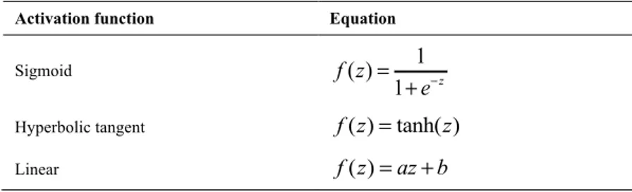
The most commonly used activation functions are summarized in Table 1.1. In this thesis we adopted an MLP neural network to forecast the energy consumption in a building, as better explained in Chapter 6.

Table 1.1. – Some common activation functions.

Activation function Equation

Sigmoid _{( )} 1 1 z f z e− = +

Hyperbolic tangent f z( ) tanh( )= z

Linear f z( )=az b+

1.4.1 The backpropagation training algorithm

The most popular training technique of an MLP network is the well-known

backpropagation training algorithm [131], a supervised learning technique that

looks for the global minimum of the error function in the weight space using the method of gradient descent.

The idea is to present the network a set of matched input and desired output patterns, called training set. The output given from the network for each training pattern is compared with the desired output, by evaluating the error. This error is used to adjust the weights in the network so as to reduce the overall error of the network.

is repeated many times until the output of the network produces a satisfactory error. Then, the weights are held and from now on the trained network is able to generalize and correctly answer to new, unseen input data.

The combination of weights which minimizes the error function is considered to be a solution of the learning problem.

The backpropagation algorithm can be executed in two versions: online or batch, dependently on the way the network weights are adjusted. In the former, the weights are adapted after each pattern has been presented to the network, while in the latter, they are adapted at the end of each epoch.

The backpropagation algorithm is the most computationally straightforward algorithm for training the multilayer perceptron [49]. Some problems may occur during the training, thus they will be briefly described below.

The network may be trapped in a local minimum of the error function.In fact, the error surface can contain more than one minimum, i.e., a global minimum and a few local minima. Two learning parameters (learning rate and momentum) should be adjusted in order to avoid the problem. The parameters act on the step size used during the iterative gradient descent process.

Another kind of problem that may occur during the training of a neural network is

overfitting. It occurs when the error on the training set is very small, while the error

on some new patterns not presented during training is extremely large. The reason for this is that the network has learned perfectly the training examples, but has not learned how to generalize, thus the error on new data easily grows.

The solution to this problem is the early stopping method: this method trains the network with only a part of the available data (training set), while the remaining data are split into two sets, namely, validation set and test set. During the training process, patterns from the training set are used to update the weights in the usual way, while patterns from the validation set are presented to the network to check its generalization capability when the training is still in progress. As soon as the error on the validation set starts to grow, and continues to grow for a given number of epochs, it means that overfitting has started, so the training is stopped and the weights corresponding to the minimum validation error, before the occurrence of

overfitting, are held.

Finally the generalization capability of the trained network is tested on the test set.

1.5 Neural networks for time series forecasting

Prediction or forecasting is a special type of dynamic filtering in which past values of one or more time series are used to predict future values of the unknown time series. Formally, a time series is a set of values that describes the evolution of a phenomenon over time, stemming from a process for which a mathematical description is unknown. Thus, usually the future behavior of a time series cannot be exactly predicted, indeed, it can be estimated [41].

Several mathematical models are present in the literature to solve prediction problems, such as regression analysis [29, 56, 81], time series analysis [57], and neural networks [9, 96, 138].

In time series modeling, the Non-linear Auto-Regressive model with eXogenous

inputs (NARX) is an important class of discrete-time non-linear systems, where the

current value of an unknown (endogenous) time series is related to the past values of the same series, and to the current and past values of the exogenous (independent) time series. More in detail, this model allows to forecast the future values of the output time series y(t), knowing the past values of the same endogenous series y(t) and the past values of the exogenous series x(t). The equation model is the following:

( )

( ( 1),..., (

), ( 1),..., (

))

y t

=

f x t

−

x t d y t

−

−

y t d

−

where, x(t-i) and y(t-i) denote the exogenous input and the output of the model at a previous discrete time step i, respectively, and dx and dy denote the maximum

delays considered for the two time series. Though these values can be different for the two time series involved, usually dx = dy = d is the preferred choice.

The NARX model can be implemented in open loop mode or closed loop mode. In the open loop mode, the system computes the output without using the feedback. Generally, to obtain a more adaptive control, it is necessary to feed the output of the system back as input. This type of system is called a closed loop system.

Figure 1.4 shows the model block diagram in closed loop mode. This means that the output of the system is fed back as input.

Figure 1.4. – NARX model block diagram in closed loop mode.

The NARX model is one of the most general time series analysis models [87, 88], as it is the straightforward generalization of the linear Auto-Regressive (AR) model to the non-linear case.

In Equation (1.2), the forecast horizon, i.e., the number of data points to be forecasted, is equal to one. The prediction can also involve several steps ahead. If the time horizon is greater than one, two different forecasting schemes exist: i) an

iterative scheme, which aims to predict a variable at a given time step and the

obtained prediction is used as input for the forecasting of the next time step; ii) a

direct scheme, which aims to predict the next n time steps from the same input data

[145].

The time series prediction process usually involves 5 steps [41]:

1. preprocessing of the data: perform smoothing or normalization, remove the outliers;

2. identification of the model: select the architecture, set an appropriate number of layers and hidden neurons for each layer, set learning parameters values;

3. training of the network (usually in open loop mode);

4. validation of the trained network: compute the error, check the prediction ability of the network;

5. use of the network for forecasting (usually in closed loop mode).

Regarding previous step 4, several metrics exist to evaluate the error and the goodness of the network.

The most frequently used are: the Mean Absolute Percentage Error (MAPE), the Mean Square Error (MSE), the Root Mean Square Error (RMSE). To assess the goodness of the forecasting model, also the coefficient of determination R2 _{can be}

used. It indicates how well a regression line fits a set of data. It provides a measure of how well future outcomes are likely to be predicted by the model. R2 _{near 1}

indicates a good fitting of the model to the data, R2 _{closer to 0 indicates bad fitting.}

The following equation expresses the coefficient of determination:

2 2 1 2 1

ˆ

(

)

1

(

)

x

x

R

x

x

−

= −

−

∑

∑

where, n is the number of data, xi and

x

ˆ

data, and x is the mean of the actual data.

The numerator is called residual sum of squares and it is a measure of the variability of the forecasting error. The denominator is called total sum of squares and measures how much variation there is in the data (with respect to their mean value).

1.5.1 The NARX neural network

ANN models may be used as alternative methods to autoregression models in engineering analyses and predictions [77, 92]. Thanks to their ability to model complex non-linear functions or unknown functions by learning from examples, neural networks are particularly suited to implement NARX models.

A NARX neural network is the network used to implement a NARX model. It is a special kind of Time Delay (TD) neural network, i.e., a feed-forward network with a tapped delay line associated with inputs and output, particularly suited to time-series prediction.

The non-linear function f of Equation (1.2) is generally unknown and can be approximated, for example, by a neural network. The resulting architecture is then called a NARX neural network and it is shown below in Fig. 1.5.

Considering Fig. 1.5, the output of the neural network is the predicted next value in the output time series, computed as a function of the exogenous time series and

the output time series, which is fed back as endogenous input to the network. Two delays are used on both the time series. The hidden layer presents ten neurons. The associated model equation is

y t

( )

=

f x t

( ( 1), (

−

x t

−

2), ( 1), (

y t

−

y t

−

2)).

Figure 1.5. – The scheme of a simple NARX neural network (the figure was produced in the Matlab®

environment).

In this thesis we adopted a NARX neural network used with the iterative scheme to forecast the energy production in a photovoltaic installation, as better described in Chapter 4.                            

2

Fuzzy systems

2.1 Introduction

Fuzzy systems (FSs) are methodologies based on fuzzy set theory to represent and process linguistic information and have been introduced by Zadeh [164].

The mathematical theory of fuzzy logic is used to simulate the process of human reasoning, i.e., approximate reasoning. Fuzzy logic is an extension of classical logic (in which any statement is either true or false) where several degrees of truth are allowed [22]. A fuzzy set is a generalization of a classical set in which the membership function is a continuous function with values in the interval [0, 1] in place of two discrete values {0} and {1} of a classical set.

A set of fuzzy rules is used to specify an input-output mapping between the input variables (i.e., linguistic variables) and the output class.

Each rule is represented as a conditional statement of the kind “if premise then consequence”, where the premise and the consequence are expressed in terms of fuzzy sets and linguistic variables. Rules are usually fixed basing on some expert’s previous knowledge, or drawn directly from data. In fact, extracting fuzzy rules from data allows modeling the relationships existing in the data by means of if-then rules that are easy to understand, verify and extend [24].

Let us now spend a few words about the main benefit of fuzzy systems: interpretability. Sometimes it is interesting not only to have an accurate classifier at our disposal, but also to have an easily interpretable classifier capable to let understand its operating (“white box” model). For this reason fuzzy systems are widely adopted in real-modeling problems where vagueness and uncertainty can be represented by using linguistic variables, instead of classical variables, thus obtaining more interpretable results.

However, not all the fuzzy classifiers are necessarily interpretable. According to the recent literature [7, 109], there are many concerns to be addressed and constraints to be included during the design stage to guarantee interpretability. Typically, interpretability of fuzzy rules depends on three issues: i) the fuzzy partition should be both complete and distinguishable (i.e., understandable linguistic terms should be easily assigned to the fuzzy sets of the partition); ii) the fuzzy rules in the rule base should be consistent, i.e., there should not be any conflicting rules; iii) the number of variables in the rule premise should be as small

as possible [94].

Fuzzy systems have been applied to a wide variety of fields ranging from control, signal processing, communications, classification and soft computing.

The chapter has the following outline. Section 2.2 recalls the main concepts of fuzzy classifiers, while Section 2.3 presents the Fuzzy Rule-Based Classifier (FRBC) employed in this work, i.e., the generation of the rule base from data and the fuzzy inference method adopted.

2.2 Overview of Fuzzy Rule-Based Classifiers

Fuzzy rule-based classifiers (FRBCs) consist of two main components: the Knowledge Base (KB) and the Fuzzy Reasoning Method (FRM). The KB is made up by a Rule Base (RB) and a Data Base (DB). The former contains a set of fuzzy if-then rules, while the latter contains the semantic parameters of the fuzzy sets that model the linguistic variables used in the fuzzy rules. Each rule specifies a subspace of the pattern space using the fuzzy set in the antecedent part in the rule. The FRM maps any input pattern X to its predicted class C using the information provided in the KB. An FRBC scheme is represented in Fig. 2.1.

Figure 2.1. – A fuzzy rule-based classifier.

The design of a FRBC consists basically in finding a compact set of fuzzy if-then classification rules derived from human experts or from domain knowledge, able to model the input-output behavior of the system. The next step is to combine these rules in order to associate a given input to a single conclusion which is the output.

In the following we show three typical formulations of fuzzy if-then rules for classification.

Let us consider an M-class classification problem related to M classes

{ }

C

an F-dimensional input space, and a set of (F+1) fuzzy partitions ( ₁f,..., f_f)

f Q

P = A A ,

f=1,…(F+1), on F input variables X1,…,Xf and one output variable X(F+1); each

partition consists of Qf membership functions. Moreover, let { , } 1

t t N

t

o ₌

input-output pairs to be classified, where ( ,...,₁t t ) F

x x is the feature vector associated with pattern _xt_{, and o}t _{the associated class index.}

Under the previous assumptions, an FRBC rule base made of a set of L rules

1

{ }L

k k

R ₌ can be expressed in different ways. In the next we report the three most common kinds of rules used for pattern classification problems [30]:

i) fuzzy rules with a single consequent class:

,1 , ,( 1) 1 1 ( 1) : _k ... F_{k F k F} , k F F R ifX is A and X is A_{δ δ} thenX ₊ is C_{δ +} (2.1)

where k is the rule index, δ is the index of the fuzzy set to be used for _{k f,} variable f in rule k, f = (1,…, F), and

C

+ means that the output class

associated with rule k is the one having index δ_{k F,(} +₁₎;

ii) fuzzy rules with a single consequent class and a single certainty factor (SCF) γ_k, i.e., the weight associated with the rule, with a value in the interval [0, 1]: ,1 , ,( 1) 1 1 ( 1) : ... ; k k F k F F k F F k

R ifX is A and X is A_{δ δ} thenX + is C_{δ +} with

γ

iii) fuzzy rules with multiple consequent classes and multiple certainty factors (MCF) j k γ (j = 1,…, M): ,1 , 1 1 1 ( 1) 1 : ... ... ... . k k F F M k F F M k k

R if X is A and and X is A_{δ δ} then X ₊ is C C with γ γ (2.3) The degree of satisfaction

,

, ,k f k t fδ

µ of the generic condition “

, k f f f

X is A_δ ”, corresponding to pattern _xt_{, is computed in the same way for the three kinds of} rules, as the membership function value associated with fuzzy set

, k f f A_δ , in the f-th component x :tf ,,k f_, k f_, ( ) k t f t fδ Aδ xf µ = .

2.3 The implementation of a FRBC:

frbc

In this thesis, we will consider only rules with a single consequent class and a single certainty factor (see Equation (2.2)), which represents the certainty degree of the classification in the specified class for an input pattern belonging to the fuzzy subspace identified by the rule antecedent. These rules provide the best tradeoff between flexibility and complexity. Furthermore they naturally fit the Matlab® Fuzzy Logic Toolbox (FLT) rule base structure.

The FRBC used in the present thesis, presented in [28] was developed under the Pattern Recognition Toolbox (PRTools) [42], the de facto standard toolbox for classification in Matlab®_.

frbc follows the PRTools base philosophy, e.g., use of

fast and heuristic-based training algorithms, function reuse, powerful and concise syntax, automatic training from data, total compatibility with the Matlab®

environment. A brief description of PRTools framework and the instructions on how to implement a new classifier in PRTools are presented in Appendix A, and

supporting material can be found in [42, 151].

In the following sections we explain the method employed to automatically learn the KB form data and the general model of fuzzy reasoning used.

2.3.1 The rule base construction

The main issue in the development of fuzzy classifiers is the proper training, that is, the creation of an efficient rule base. The rule base can be derived from the expert previous knowledge or more easily can be derived directly from numerical input-output pairs. In the literature, many approaches have been proposed for generating fuzzy rules from numerical data, such as heuristic approaches [2, 70, 93], neuro-fuzzy techniques [103, 110, 111, 112, 150], clustering methods [3, 130], and genetic algorithms [19, 51, 68, 73].

In order to meet the PRTools base philosophy (see Appendix A), we are interested in existing batch-mode oriented approaches to automatically generate fuzzy rules from data, that are well-assessed and widely accepted, that need few free parameters to be specified, and that are associated with fast heuristic training methods. In our opinion, among the approaches existing in the literature, the technique that best meets these requirements is the Wang and Mendel method extended to classification problems, an adaptation of the well-known Wang and Mendel method for regression problems [154]. This method assumes that the fuzzy partitions of the input and output variables are provided by the user. A typical and easy way to achieve this is to resort to uniform fuzzy partitions consisting, for input variables, of a limited number of fuzzy sets, while, for output variables, of as many fuzzy sets as there are classes. So, the Wang and Mendel method is the training technique available in frbc [28]. This method seems to be simpler and with less construction time than a comparable neural network, maintaining the comparability of the results [106]. In addition, it allows to combine in the same framework both numerical and linguistic information [154].

In the following, the formal steps of the Wang and Mendel algorithm extended to classification problems are briefly introduced:

STEP A. generate a uniform fuzzy partition of the input domain, made of Qf, f= 1,…, F, fuzzy sets for each input variable f (usually Qf = Q = 3, 5, 7 or 9);

STEP B. generate a uniform fuzzy partition of the output variable, made of M fuzzy sets (one set for each class);

STEP C. generate an initial raw rule base (one rule for each training pattern);

STEP D. remove duplicated rules; STEP E. compute certainty factors;

STEP F. remove conflicting rules (i.e., rules having the same if part but different then parts) by keeping, for each set of conflicting rules, only the rule with the highest CF.

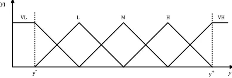
More in detail, this algorithm generates the fuzzy rule base assuming a uniform fuzzy partition for the input variables. Thus, the domain of each input variable is divided into Q=2N+1 regions, typically N∈{1, 2,3, 4} (STEP A). The length and the number of the regions may be different for the considered variables. A fuzzy membership function is then defined for each region. Typically this function has its maximum value in the middle point of the region and assumes its minimum value in the central points of the two neighboring regions, although different definitions are possible. Figure 2.2 shows an example of a fuzzy partition built according to the Wang and Mendel approach, on a generic variable y whose domain interval [y-, y+] has been divided into Q=5 regions (N=2).

Doing so, the thresholds identify a grid on the input variable space. So, for instance, if we have two input variables and we define two evenly spaced

thresholds for each variable, we obtain a uniform 9-area grid.

y

µ(y)

y$ y+

VL L M H VH

Figure 2.2. – An example of a fuzzy partition for the input variables, built according to the Wang and

Mendel approach.

Regarding STEP B, the fuzzy sets used to represent the output partition are usually fuzzy singletons, as we deal with a classification problem. Since each data pair generates a fuzzy rule in the rule base (STEP C), there will possibly be some duplicate rules and some conflicting rules, i.e., rules having the same if parts but different then parts. The duplicated rules are simply deleted (STEP D), while to solve a conflict, a CF is assigned to each conflicting rule of a set. The CF is defined so as to take into account the importance of each rule in the entire rule base (STEP E). The winning rule, within a conflicting set, is the one that has the maximum CF. The other rules of the set are discarded (STEP F).

From the field of data mining [5], the CF is tipically computed as the confidence of the fuzzy association rule

k

k

A

⇒

C

then k

C_δ , where Ak represents the antecedent part of the fuzzy rule, and C_δk the

class appearing in the consequent. The CF is calculated as follows:

, , :t 1 , k N k t k t k t classC_δ t

γ

∑

∑

where _Ωk t, _{is the strength of activation of the antecedent of rule R}

k for the t-th

pattern, and N is the number of training patterns.

However, in past research, many heuristic measures have been proposed to specify the weight of a fuzzy classification rule [72, 93, 166]. Nozaki et al. [115]

proposed a method of learning rule weight using Reward & Punishment, in which, considering the classification of a pattern using the single winner FRM, the weight of the winner rule is increased or decreased depending on whether the pattern has been correctly classified or not. In other relevant methods [66, 72], the computation consists of two phases. First, the certainty factor is calculated as the confidence of the fuzzy rule (as in Equation (2.4)), then, the certainty factor is refined with a measure that depends on the specific method, with the aim to improve the classification performance.

We recall that any shape and number for membership functions can be selected. Clearly, the higher the number of membership functions, the bigger the accuracy obtained. On the other hand, a large number of membership functions leads to a large rule base dimension and, consequently, to a higher complexity.

2.3.2 The fuzzy reasoning method

The FRM available in frbc [28] for MCF rules is a general model of fuzzy reasoning for combining information provided by different rules. It is an extension presented in [30] of the fuzzy classifier defined by [82].

In the following, we recall the steps of the FRM applied to each input pattern

x

antecedent, say matching degree;

STEP 2. compute, for each rule, the association degree of the pattern with the class specified by the rule;

STEP 3. compute, for each rule, the stressed association degree by emphasizing the association degree;

STEP 4. determine the soundness degree of the classification of the pattern

x

STEP 5. assign pattern

x

For each step of the inference process, several operators can be selected, thus giving origin to different inference methods.

In particular, as regards STEP 1, the matching degree Ω for pattern

x

is calculated as the AND operator (any T-norm) between the membership function values: , , , 1 ,k f, 1,..., , 1,..., . k t F k t f= µfδ k L t N Ω =I = = (2.5)

The AND operators available in frbc are the minimum and the product.

In STEP 2, the association degree is computed by applying a combination operator h to the matching degree _{Ω and the certainty factor γ}k t,

k as follows

(possible choices for h are product and minimum):

, ₍ ,_{, ), 1,..., , 1,..., .}

k t k t

k

In STEP 3 the association degree is stressed by applying a stress function g so as, e.g., to increase higher values and decrease lower ones:

, ₍ ,_{), 1,..., , 1,..., .}

k t k t

B =g b k= L t= N (2.7)

We have considered two stress functions, namely No_Stress function g1 (identity

function) and Square_SquareRoot function g2, as defined hereafter:

1( ) [0,1] g z = ∀ ∈z z (2.8) 2 2 0.5 ( ) 0.5 . z if z g z z if z ⎧ < ⎪ = ⎨ ≥ ⎪⎩ (2.9)

In STEP 4, the soundness degree ˆt j

o associated with each output class j is computed by applying an aggregation function Γ to the Stj positive association

degrees s t, j a : ,

ˆ

(

),

1,..., ,

1,...,

o

= Γ

a

s

=

S j

=

M

We have considered seven different aggregation functions (maximum, normalized addition, arithmetic mean, quasi-arithmetic mean, Sowa and-like, Sowa or-like, Badd operator). Table 2.1 shows the mathematical equations of the aggregation functions [30]. For each function we indicate the value of the free parameter (if existent) used in the experiments.

In particular, the use of the maximum operator leads to the implementation of the classical FRM, which classifies a new example with the consequent of the fuzzy rule with the greatest degree of association. Although it is used by the majority of FRBCs, it loses the information provided by other rules.

Finally, STEP 5 computes the predicted class index ˆ_{o , associated with pattern} t t

x

In the present thesis, frbc has been employed to forecast the energy production from a solar photovoltaic installation in order to help the manager of the installation in the control and the dispatch of the energy in the electrical grid, as better described in Chapter 5.

Table 2.1. – Mathematical equations for the aggregation functions.

Aggregation

function Mathematical equation

Value of free parameter Maximum max{ ... }_1... 1 t j MAX _{j= M} a as Γ = - Normalized addition _1... 1 max t t j j s s NORMADD i _{j M} i i i a a = = Γ =

∑

∑

∑

∑

Sowa and-like ΓSOWAAND=α ⋅min{a1...astj}+ (1−α)⋅ΓARIMEAN ,

[0,1]

α ∈ _{α =0.5}

Sowa or-like max{ ... } (11 t ) ,

j SOWAOR α a as α ARIMEAN Γ = ⋅ + − ⋅Γ α ∈[0,1] _{α =0.9} Badd operator 1 1 1 , t t j j s s p p BADD i i i i a + a p R = = Γ =

∑

∑