UNIVERSITÀ DEGLI STUDI DI ROMA
"TOR VERGATA"
FACOLTA' DI ECONOMIA
DOTTORATO DI RICERCA IN
Teoria Economica e Istituzioni
CICLO DEL CORSO DI DOTTORATO
XXI
Titolo della tesi
Optimal Taxation in R&D Driven Endogenous Growth Models
Nome e Cognome del dottorando
Xin Long
A.A. 2009/2010
Optimal Taxation in R&D Driven Endogenous
Growth Models
Author: Xin Long
PhD Program: Economic Theory and Institutions (Cycle: XXI)
Academic Year of Thesis Discussion: 2009/2010
Supervisor: Alessandra Pelloni
Coordinator: Luigi Paganetto
Version: December 10, 2009
Abstract
Is it possible to increase growth and welfare by raising lump-sum taxes and disposing of the tax revenues? Is it possible to increase welfare by raising capital income taxes and redistributing the revenue as a subsidy to labor income? This thesis shows these may indeed be the case in standard R&D models with technological change, represented either by an increase in the variety of intermediate goods or by creative destruction. The key mechanism is that with elastic labor supply the tax programs can increase the employment rate in equilibrium. This creates two spillover e¤ects on the R&D pace. In addition the tax programs themselves will have level e¤ect on the instantaneous utility. The relative momentums of the spillovers and the level e¤ect determine the sign of the welfare e¤ect. It is shown that, for parameter values consistent with available estimates, the growth and welfare can both be improved under the wasted lump-sum tax program, and that the welfare e¤ect can be positive even if the long-run growth rate decreases after the increase in the capital income tax rate.
JEL Codes: E62, H21, O41
Keywords: R&D, endogenous growth, lump-sum taxes, capital income taxes, labor income subsidy, growth e¤ect, welfare e¤ect, optimal tax rate.
I would like to thank my supervisor, Alessandra Pelloni, for her heuristic guide. And I would also like to thank Robert Waldmann, for his very useful suggestions. All errors are the author’s. Contact: Xin Long, Faculty of Economics, University of Rome "Tor Vergata", Via Columbia 2, 00133 Rome, Italy, [email protected].
Contents
Introduction ……….………...……… 1
Chapter I. Lump-sum taxes in a variety expansion model ………....…. 3
1. Introduction ………... 3
2. The model ……….…....… 7
2.1 Households ……….………..….. 7
2.2 Firms ………..……. 8
2.3 Government ……….. 10
3. Market equilibrium ………...………..… 10
4. Effects of taxes ………...……….... 12
4.1 Effect on labor ………....….…. 12
4.2 Effect on growth ………...….….. 12
4.3 Effect on welfare ………..………..….. 12
4.4 Are wasted lump-sum taxes good for reasonable parameter values? …… 14
5. Economic intuition ………..…. 18
Appendices ………..……. 20
Chapter II. Lump-sum taxes in a creative destruction model ………... 22
6. The model ……….………....….. 22
6.1 Final good sector ……….…...….. 23
6.2 Intermediate good sector ………..….... 24
6.2.1 Production ……….…... 24
6.2.2 R&D Activity ……….….. 25
7. Market equilibrium ……….…………....… 27
8. Effects of taxes ………..………... 29
8.1 Effect on labor ………..………..….. 29
8.2 Effect on growth ……….……….. 30
8.3 Effect on welfare ………..…………..….. 30
8.4 Are wasted lump-sum taxes good for reasonable parameter values? …... 31
Appendices ………..……..…. 36
Chapter III. Capital income taxes in a variety expansion model ……….…. 38
10. Introduction ………..…….... 38
11. The model ………..……... 41
11.1 Households ………..…………... 41
11.2 Government ………..……….. 41
12. Market equilibrium ……….……….. 41
13. Effects of taxes ………..……... 43
13.1 Effect on labor ……… 43
13.2 Effect on growth ………...… 44
13.3 Effect on welfare ………....… 45
13.4 Are capital income taxes good for reasonable parameter values? …..…… 47
14. Comparison between the market economy and the social planner’s economy..50
15. Economic intuition ………..…..…... 53
Appendices ………..…..…. 55
Chapter IV. Capital income taxes in a creative destruction model ………... 56
16. Introduction ………..…… 56
17. Market equilibrium ……….….……. 57
18. Effects of taxes ………..…………... 60
18.1 Effect on labor ………..…….. 60
18.2 Effect on growth ………... 61
18.3 Effect on welfare ………..…….. 63
18.4 Are capital income taxes good for reasonable parameter values? …....….. 65
19. Comparison between the market economy and the social planner’s economy..68
20. Economic intuition ………..…………. 72
Appendices ………..………... 73
Conclusion ……….……….….. 77
Introduction
The prediction that permanent variations in tax rates would give rise to dif-ferent steady-state growth rates has long been a hallmark of the endogenous growth literature. In contrast to the older neoclassical framework, where long-run growth was exogenously determined by the rate of technical progress, these models predict that increases in tax rates would induce lower growth rates (see, for example the survey in Myles (2000) and Jones and Manuelli (2005)). This negative correlation re‡ects the distortional e¤ects of taxation. However, empir-ical cross-country growth studies, notably by Levine and Renelt (1992), Levine and Zervos (1993) and Tanzi and Zee (2000) have not been able to con…rm this negative correlation; and more recently Angelopoulos et al (2007) even shows contrary conclusion. Jones (1995) and Stokey and Rebelo (1995) also argued that US time series data was at odds with the implications of linear growth models: on the basis of these models, the dramatic increase in income taxation which took place in the early 1940s would have been expected to contempora-neously decrease the US per capita growth rate, but this did not appear to be the case.
Within the endogenous growth literature, in particular many studies focus on R&D activities, a major driving force for growth, and to …scal incentives for these activities, which are subsidized in many industrial countries. However, there are some common limitations of these studies. One limitation is that they often treat labor supply as inelastic, thereby abstracting from the decision to allocate time between work and leisure. Since the labor-leisure choice is actual microeconomic phenomenon - individual agents face the tradeo¤ and make their decision in time allocation, I adopt the labor-leisure choice into my model for the household sector in the economy to show a non obvious result for …scal policy based on the intratemporal tax distortions. Another limitation is that they often analyze only the e¤ect of the taxes on growth without further looking into their in‡uence on welfare by implicitly assuming that higher growth rate always leads to higher welfare. But in an imperfectly competitive dynamic economy this assumption cannot always be justi…ed because that the growth rate in a decentralized economy may di¤er from the socially optimal rate and if the former is bigger than the latter, the increase of the former may decrease overall welfare in stead of raising it. Another reason that can nullify this assumption is that the change in instantaneous consumption and that in growth rate may counteract each other in determining the utility level, so even if growth rate increases but if it can be o¤set by the decrease in the instantaneous consumption, the overall welfare may still be reduced. Therefore, it leads to the necessity of the analysis of both growth e¤ect and welfare e¤ect in my study.
An important debate in the literature of R&D driven endogenous growth model is over with-or-without scale e¤ect. The very baseline endogenous tech-nological change models feature a scale e¤ect in the sense that a larger popula-tion, L, translates into a higher interest rate and a higher growth rate. Jones, among others, suggest modi…ed versions, where the scale e¤ect can be removed
but higher population growth can still translate into higher per capita output growth. Following the line of research that puts technological innovation at the forefront of explanations of di¤erences in standards of living across countries and time, I use the endogenous growth models as in the Chapter 6 and 7 of Barro and Sala-i-Martin (2004) to emphasize features of the real world like imperfect competition, accumulation of intangibles, economies of scale, creative destruc-tion, and the distinction between quality improvements and the creation of new products. Thus my model incorporates scale e¤ect in the sense that a greater e¤ective labor force, embodied by longer equilibrium working hours assigned to representative agents with an aggregated scale of unit, creates more demand for intermediate goods, making R&D more pro…table thus leads to faster growth. But what I am doing does not give answers to the relevant criticisms over either side of the debate, because we cannot assume that the e¤ect of an increase in the number of workers is just the same as an increase in hours worked per worker, on which we focus.
I do not incorporate the variety expansion and creative destruction into a complicatedly comprehensive model for reasons such as that simpler model allows for easy analytical solutions to reaching the optimal welfare e¤ects of the interested policy variables, and that the parallel models give qualitatively the same insights into the real economy as the comprehensive model does, and further clearly show the di¤erent momenta of the e¤ects of the taxes whereby I can tell which economic externality the taxes can take e¤ect on by the most.
The other characteristics of my model can be brie‡y summarized as follows: Representative agent with in…nite life: this enables me to study the welfare e¤ects of the taxes without considering any distribution e¤ect.
Balanced …scal budget: this avoids consideration on the public expenditure …nanced by de…cits and simpli…es the analysis by excluding the intertemporal distribution e¤ect of taxes (subsidies).
No productive use of the taxes: this allows me a closer view of the e¤ect of …scal policy.
No capital accumulation: no capital in the usual neoclassical sense of a homogenous, durable, intermediate good accumulated through foregone con-sumption. Instead, there are di¤erentiated, non-durable, intermediate goods produced through foregone consumption. One can think of these goods as cap-ital, albeit with 100% instantaneous depreciation. This structure allows me to simplify the model with no consideration on the e¤ect of capital accumulation on growth without loss of generality for the purpose of my research.1
The …scal policy variables within the interest of research are the lump-sum taxes and the capital income taxes. I choose to study these two taxes because in the optimal taxation literature, the lump-sum taxation (subsidy) are usually considered non-distortionary so taken as the …rst-optimal policy instrument but it is not the case in my model, and researches on optimal capital income taxation
1As Judd points out, much of the intuition behind the literature on optimal taxation of
capital stems from the property that capital income is construed as the income to suppliers of the homogeneous (durable) intermediate good. Thus my model complements his point.
diversify generically in their conclusions thus it leaves much room for reexami-nation. In the following charpters I will further review the related literature in detail.
My analysis focuses on three aspects. First, I discuss the steady-state equi-librium and analyze the characteristics of the equiequi-librium, i.e. the determinacy or indeterminacy of the balanced growth path. Second, I derive the e¤ects of the taxes on the long-run labor-leisure allocation and the long-run changes in growth rate. Particular attention is devoted to the welfare of the representative agent as represented by the present value of the bene…ts. Third, I calibrate the model to a benchmark economy and assess the numerical e¤ects of these taxes relative to this benchmark. And through sensitivity analysis I show the bene…-cial e¤ect of the taxes on welfare for plausible values of parameters. Finally, I analyse the social planner’s economy and compare it with the market economy to show that the …scal policies a¤ect welfare in a second-best way.
My main conclusions are the following:
There are no transitional dynamics and the balanced equilibrium is deter-minate and Pareto suboptimal.
Lump-sum taxes, whose revenues are thrown to ocean, may increase long-run growth rate as well as welfare.
Capital income taxes, whose revenues are returned to labor, may improve welfare even if they reduce long-run growth.
Values of the economic parameters in‡uence not only the direction but also the magnitude of the policies’welfare e¤ect, and thus determine the variant levels of optimal tax rates.
The thesis is organized as follows: in chapter 1 and 2 a variety expansion model and a creative destruction model are set up respectively, and the e¤ects on growth and welfare of the lump-sum taxes are studied in the two models; chapter 3 and 4 are devoted to the analysis of capital income taxes also in the respective models, with the studies on social planner’s solution followed each. In the end the conclusion is given.
Chapter I. Lump-sum taxes in a
variety expansion model
1
Introduction
In this charpter I show a non obvious result for …scal policy that is made possible by allowing for ‡exible labor supply in R&D models: the fact that lump-sum taxes can have positive e¤ects on growth even when the revenue is not used in a productive way.
It should be certainly possible to return the revenue to agents in such a way as to increase their welfare. However assuming as I do that the revenue is not
returned allows me a closer view of the e¤ect of …scal policy. In particular it is often found in theoretical models that growth can be increased by subsidies to R&D …nanced through lump-sum taxes (see for example Barro and Sala-i-Martin (2004), chapter 6, or Zeng and Zhang (2002)). Here I show that with a ‡exible labor supply, lump-sum taxes can in themselves increase growth and welfare, i.e. have a direct e¤ect on them.
I conduct my study by using a standard model of endogenous technological progress with an in…nitely lived representative agent, originally proposed by Rivera-Batiz and Romer (1991) and known as the "lab-equipment model", and presented in Barro and Sala-i-Martin (2004), chapter 6. Given its ‡exibility and simplicity this model provides a tractable framework for analyzing a wide array of issues in economic growth.2 Entrepreneurs spend a …xed cost in order to
develop new intermediate goods. Each chooses to produce the same amount of each intermediate good. Output in the …nal goods production sector is linear in the number of intermediate goods used so unbounded growth is possible. The basic di¤erence in assumptions with respect to this benchmark model is that the decision to supply labor is explicitly analysed.
I analyse the long-run e¤ects of a lump-sum tax whose proceeds are thrown away and …nd that such a tax will increase growth and will increase welfare for a plausible region of the parameters space. The intuition is simply that in my model, lump-sum taxes have an impact on the allocation of resources, because they in‡uence labor supply and consequently the rate of return on capital and the rate of growth. In the example which I consider, the income e¤ect of a wasted lump-sum tax causes households to consume less leisure and supply more labor. This causes an increase in the interest rate and the long-run rate of growth. Put more explicitly, the mechanism which is at work is the following: a lump-sum tax induces a negative income e¤ect thereby inducing agents to work more; more employment raises the returns to the R&D activity; growth is therefore increased.
The reasoning of the present study is inevitably involved into the debate of with-or-without scale e¤ect associated with the endogenous technological progress models. As stated before, the very baseline models feature that a larger population, L, translates into a higher interest rate and a higher growth rate. However, this is problematic for three reasons as argued in a series of papers by Charles Jones and others:
(1) Larger countries do not necessarily grow faster (though the larger market of the United States or European economies may have been an advantage during the early phases of the industrialization process).
(2) The population of most nations has not been constant. If we have popula-tion growth as in the standard neoclassical growth model, e.g., L(t)=exp(nt)L(0), these models would not feature balanced growth, rather, the growth rate of the economy would be increasing over time.
(3) In the data, the total amount of resources devoted to R&D appears to
2See the excellent survey in Gancia and Zilibotti (2005) for a selection of the wide range
increase steadily, but there is no associated increase in the aggregate growth rate.
These observations have motivated Jones (1995) to suggest a modi…ed ver-sion of the baseline endogenous technological progress model. In that model the scale e¤ect can be removed by reducing the impact of knowledge spillovers. While this pattern is referred to as "growth without scale e¤ects", it is useful to note that there are two senses in which there are limited scale e¤ects in these models: First, a faster rate of population growth translates into a higher equi-librium growth rate. Second, a larger population size leads to higher output per capita. It is not clear whether the data support these types of scale e¤ects either. Put di¤erently, some of the evidence suggested against the scale e¤ects in the baseline endogenous technological change models may be inconsistent with this class of models as well. It is also worth noting that these models are sometimes referred to as "semi-endogenous growth" models, because while they exhibit sustained growth, the per capita growth rate of the economy is determined only by population growth and technology, and does not respond to taxes or other policies. Some papers in this literature have developed models of endogenous growth without scale e¤ects, with equilibrium growth responding to policies, but this normally requires a combination of restrictive assumptions (see, among others, Dinopoulos and Thompson (1998), Howitt (1999) and Young (1998)). And further, Aghion and Howitt (1998) and Ha and Howitt (2007) argue that semi-endogenous growth models along these lines also face di¢ culties when con-fronted with the time-series evidence.
In fact, each one of the above arguments against scale e¤ects can be debated. Some argued that looking at the 20th century data may not be su¢ cient to reach a conclusion on whether there is a scale e¤ect or not. Kremer (1993) argues, on the basis of estimates of world population, that there must have been an increase in economic growth over the past one million years. Laincz and Perreto (1996) argue that R&D resources allocated to speci…c product lines have not increased. Others argued that countries do not provide the right level of analysis because of international trade linkages. These can be seen in the survey of Acemoglu (2009). In addition, a more recent research, Samaniego (2007), reconciles the presumption that R&D is a key driver of economic growth and the empirical evidence by showing that R&D contributes to growth through investment-speci…c technical change instead of directly forming the total factor productivity (TFP) change. In this way, the empirical "puzzles", including the weak link between measures of knowledge and productivity, and the estimates pointing to the presence of constant or even increasing returns to the production of ideas (which has counterfactual implication that rates of economic growth should increase with the population size), can be easily reconciled.
My model incorporates scale e¤ect in the sense that a greater labor force creates more demand for intermediate goods, making R&D more pro…table so that a greater labor force leads to faster growth. I do not deliberately remove the scale e¤ect not only because that the models "without scale e¤ect" them-selves meet unsolved problems, but also because that in fact, the "knife-edge" assumptions in those models imply that the responsiveness of long-run growth
with respect to policies results at least partly from the inclusion of the scale of labor supply into the factors determining per capita output growth. This can be seen in the survey of Jones (1999), as in Howitt (1999) who shows that while population growth positively a¤ects per capita output growth, population growth itself depends on the amount of labor supply. Jones (2003) also inserts that when population is endogenized, the invariance result in the models "with-out scale e¤ect", i.e., changes in the allocation of human capital to research have only level e¤ects but no growth rate e¤ects, can be overturned. Therefore, keep-ing scale e¤ect in my model can be justi…ed because it enables me to analyse how policies a¤ect the endogenous labor-leisure choice. It is worth mention-ing that our key argument, i.e., higher labor supply leadmention-ing to higher growth, varies from those proposed in the baseline endogenous technological progress models in that the e¤ective labor force in my model is represented by the work-ing hours determined by representative agents with an aggregated scale of unit. As for the set-up of my model, considering that if population was growing the economy would not admit a steady state and the growth rate of the economy would increase over time (output reaching in…nity in …nite time and violating the transversality condition), I abstract my model from population growth and standardize the scale of population to unit, following Zeng and Zhang (2007), therefore the e¤ective labor force in my model is exactly the labor-leisure choice of the representative agent, and is subject to the in‡uence of …scal policies, which is per se the interest of research of my thesis. Thus we can conclude that what I am doing does not give answers to the relevant criticisms over either side of the debate, because we cannot assume that the e¤ect of an increase in the number of workers is just the same as an increase in hours worked per worker, on which we focus.
The result of my study is an example of second-best theory. The idea that taxes whose revenue is not used productively must reduce welfare is based on the …rst-best intuition that a waste of resources has a positive social cost. How-ever the withdrawal of resources from productive use may have a social bene…t in an economy in which there is imperfect competition, i.e. in a second-best environment.
Another contribution of my analysis is the following: as said above it is very frequent in works studying the e¤ects of …scal expenditures to assume …nancing by lump-sum taxes, taken to be non distortionary, or to assume that proceeds of taxes are returned lump-sum (e.g. Devereux and Love (1995), Lin and Russo (1999), Turnovsky (2000), Zeng and Zhang (2002), or Haruyama and Itaya (2006)). However I show that, with elastic labor supply, through general equilibrium e¤ects a lump-sum tax will change relative prices and therefore be indirectly distortionary. In other words the e¤ect on growth of a tax whose revenue is returned lump-sum will be di¤erent from the e¤ect on growth of a tax whose proceeds are just thrown away and should therefore be studied separately.
The rest of this charpter is organized as follows: in section 2 the model is presented, section 3 describes the equilibrium conditions which have to hold in the model and analyses the balanced growth path characteristics of the model,
section 4 works out the labor supply e¤ect, growth e¤ect and welfare e¤ect of the lump-sum tax in the model, and does numerical calculations to show that such a tax can increase welfare for widely accepted estimates of the relevant parameters, and section 5 gives economic intuitions.
2
The model
2.1
Households
We assume that in the economy there is a continuum of length one of identical households.3 Each has utility U given by:
U = Z 1 t=0 e t 1 1 C 1 h(H) dt (1)
where C is consumption and H labor. is rate of time discount. The following conditions ensure non satiation of consumption and leisure: > 0 and
h(H) > 0, (2) (1 )h0(H) < 0. (3) Strict concavity of instantaneous felicity imposes:
(1 )h00(H) < 0 (4) and
h00h
( 1) h
02> 0. (5)
The instantaneous budget constraint consumers face is given by: _
F = rF + wH C a _ _
F . (6)
Households derive their income by loaning entrepreneurs their …nancial wealth F (of which all have the same initial endowment) and by supplying labor H to …rms, taking the interest rate r and the wage rate w as given. There are lump-sum taxes proportional to average wealth,
_ _
F , where given our normalization, F =
_ _
F . Agents, being atomistic, take these averages as variables beyond their control. In this sense these are lump-sum taxes. At an optimum, the marginal rate of substitution between leisure and consumption must equal their relative price:
h0(H)
h(H) =
w( 1)
C . (7)
3As Zeng and Zhang (2007) note, normalizing the population to unity removes from the
analysis of taxes the "scale e¤ect" discussed by Jones (1995). For a very balanced view of the debate that followed see chapter 13 of Acemoglu (2009).
Optimal consumption and leisure must also obey this intertemporal condi-tion: _ C C + h0(H) h(H)H =_ _ = r (8)
where is the shadow value of wealth. Given a no Ponzi game condition the transversality condition imposes:
lim
t!1 F exp( t) = 0. (9)
2.2
Firms
In this economy there are a …nal goods sector and an intermediate goods sector. The former is perfectly competitive, whereas the latter is monopolistic. R&D activity leads to an expanding variety of intermediate goods. All patents have an in…nitely economic life, that is, we assume no obsolescence of any type of intermediate goods.
Following Spence (1976) and Dixit-Stiglitz (1977) the production function of …rm i in the …nal good sector is given by:
Y (i) = AL(i)1 Z N
0
x(i; j) di (10)
where Y (i) is the amount of …nal goods produced and L(i) is labor used by …rm i and x(i; j) is the quantity this …rm uses of the intermediate good indexed by j. For tractability both i and j are treated as continuous variables.4 We assume
0 < < 1. The …nal goods sector is competitive and we assume a continuum of length one of identical …rms. We can then suppress the index i to avoid notational clutter. Firms maximize pro…ts given by
Y wL Z N
0
P (j)x(j)dj (11)
where w is the wage rate and P (j) is the price of the intermediate good j. By pro…t maximization we have the demand for good j given by:
x(j) = L A P (j)
1 1
(12) and labor demand by:
w = (1 )Y
L. (13)
Since the …rms in the …nal goods sector are competitive and there are constant returns to scale their pro…ts are zero in equilibrium. In contrast the …rms which
4For a discussion of the realism of the assumption as regards the intermediate products see
produce intermediate goods patent which they invent then earn monopoly pro…ts for ever. The cost of production of the intermediate good j, once it has been invented, is given by one unit of …nal good. The value of the patent for the jth intermediate good v(j; t) at time t is the present discounted value of such
pro…ts. The value of the jthpatent at time t is then
v(j; t) =
1
Z
t
(P (j) 1)x(j)e r(s;t)(s t)ds (14)
where r(s; t) is the average interest rate during the period of time from t to s. The inventor of the jthintermediate good chooses P (j) to maximize pro…ts
(P (j) 1)x(j) where x(j) is given by 12, so for each j, the equilibrium price is: P (j) = P = 1 (15) and
x(j) = x = LA11 12 . (16) Notice a higher labor supply implies a higher quantity of each intermediate goods in equilibrium. Plugging equation 16 in equation 10 gives us equation
Y = N LA11 2
1 (17)
while plugging 17 in 13 we have:
w = N (1 )A11 12 . (18) Assuming the interest rate and labor are constant over time, we have substitut-ing 15 and 16 in 14:
v(j; t) = LA11 2
1 1 1
r. (19) I will show below that if a balanced growth equilibrium exists, labor supply and the interest rate are indeed constant.
The cost of development of new products is and there is free entry in the market for inventions, so intermediate goods …rms will push the price of an invention to equate its cost and in equilibrium we will have:
r = C1L (20)
where C1 1 A
1 1
1+
1 . Notice that the higher is labor supply the higher is the interest rate, as the scales of each intermediate good are increasing in labor supply, so the entrepreneurs will be willing to pay a higher interest rate.
2.3
Government
We assume no government consumption on goods. We also rule out a market for government bonds and assume that the government runs a balanced budget. The revenue from lump-sum taxes is wasted. The government budget constraint is thus:
G = a _ _
F (21)
where on the left-hand side we have out‡ows and on the right-hand side we have in‡ows.
3
Market equilibrium
In calculating the equilibrium in the …nal goods market the total of intermediate goods used xN is subtracted from …nal production Y to obtain total value added. All investment in the model is investment in research and development of new intermediate goods N . The economy-wide resource constraint is therefore given_ by:
Y xN = C + N + G._ (22) We are now ready for the following:
De…nition 1 In a competitive equilibrium individual and aggregate variables are the same and prices and quantities are consistent with the (private) ef-…ciency conditions for the households 6, 7, 8 and 9, the pro…t maximization conditions for …rms in the …nal goods sector, 12 and 13 (or 18), and for …rms in the intermediate goods sector, 15 (or 16) and 20, with the government bud-get constraint 21 and with the market clearing conditions for labor H = L, for wealth F = N , and for the …nal good, 22.
In equilibrium the social budget constraint 22 can be written as: _
N N =
1
N(Y xN C a N ). (23) Proposition 2 If the economy follows a balanced growth path (hence BGP) variables grow at a constant rate, and in particular employment is constant at a value ~L. Along this path, rate of growth of capital and consumption, , is then given by:
= r(eL) . (24) Proof. Totally di¤erentiating 7 we get:
_ C C = _ N N + (h 0=h h00=h0) _L. (25)
From this we deduce that along a BGP, when _L = 0, the rates of growth of C and N will be the same. From 8 and _L = 0, we get 24.
In Appendix 1 I show how to deduce from the competitive equilibrium con-ditions described above the following di¤erential equation for labor, which is the fundamental dynamic equation of the model:
_ L = + 1 (h01)hL 1 r a h00 h0 + (1 )h 0 h B(L) A(L). (26) Notice that, as r is a linear function of L, 26 is a di¤erential equation in L. The denominator of the fraction on the right-hand side A(L) is always strictly positive for all values of L, by the negative de…niteness condition of the hessian of the utility function 4, so the equation is de…ned for all values of L between 0 and 1. Along a BGP _L will equal zero, so the numerator B(L) will be zero, i.e. B( ~L) = 0 where ~L is the BGP labor supply. To study the dynamic nature of a …xed point of 26, i.e. of BGP labor supply, we have to sign d _L( ~L)=d ~L, the derivative of _L with respect to L, calculated at the …xed point ~L implicitly de…ned by B( ~L) = 0. If the derivative is positive the …xed point ~L is a repeller and the BGP is locally determinate in the sense that if L were close to but not exactly equal to eL, then L would diverge further from eL. Thus, the BGP with eL a repeller is a (locally) unique equilibrium path and we can say that there is no (local) indeterminacy in this case. If the equilibrium is unstable there will be no transitional dynamics to it, the economy will always follow the BGP. If d _L(eL)=deL is negative then eL is an attractor, that is if L is near eL it will eventually approach it. So there is local indeterminacy, i.e. a continuum of equilibrium trajectories all converging to the …xed point. We have: d _dLL( ~L) =
B0( ~L) A( ~L)
A0( ~L)B( ~L) A2( ~L) =
B0( ~L)
A( ~L) (since B( ~L) = 0). Below we prove that B( ~L) = 0
implies B0( ~L) > 0. Since d _L(eL)=deL is always positive, we can deduce that if
BGP exists it is unique as from the phase diagram of 26 we can easily see that there is no way for B(L)=A(L), which is a continuous function, to cross the horizontal axis from below two times in a row.
From the instability of the equilibrium we can also deduce that there will be no transitional dynamics in the model. Below we prove that B( ~L) = 0 implies B0( ~L) > 0. We are now ready for the following:
Proposition 3 If a BGP equilibrium de…ned by B( ~L) = 0 exists, it is unique and locally determinate, so there is no transitional dynamics to it.
Proof. Since the …rst derivative of r with respect to L equals C1, we will then
have the derivative of B(L) with respect to L, deriving and rearranging:
B0(L) = C1 1 + (1 ) 1
hh00
h02 + 1 . (27)
From condition 5, we have
(1 ) 1 hh
00
h02 + 1 > (1 ) +
(1 )2
With 28, B0(L) is strictly positive: 1 + (1 ) 1 hh00
h02 + 1 > 1 + 1 > 0.
4
E¤ects of taxes
4.1
E¤ect on labor
It is relatively simple to calculate the e¤ect of taxes on labor supply in this model because the wage rate is not a¤ected by labor supply. As said above equilibrium labor supply can be expressed as the solution to B( ~L) = 0. The e¤ect of our tax program on labor can be deduced by using the total derivative of B( ~L) = 0 with respect to labor and the tax. We then have:
d ~L d a = B0( ~L) = C1 1 + (1 ) 1 hh00 h02 + 1 . (29) As we have shown above that B0( ~L) > 0, this derivative is always positive, i.e.
the increase in lump-sum tax will induce bigger BGP labor supply. This can be interpreted as a simple income e¤ect: for …xed labor supply, the tax would make households poorer so since both consumption and leisure are normal goods they consume less and o¤er more labor.
Proposition 4 An increase in the lump-sum tax rate whose proceeds are thrown to ocean will increase employment in equilibrium.
4.2
E¤ect on growth
It is easy to see that the e¤ect of the lump-sum tax on the rate of growth is positive as well, since the rate of growth of consumption increases one for one with the interest rate and the interest rate is proportional to labor supply. In detail we deduce the growth e¤ect of tax aby equation 20, 24 and 29 as follows:
d d a = @ @r @r @ ~L d ~L d a = 1 1 + (1 ) 1 hhh0200 + 1 . (30) Not surprisingly the condition for the tax to be growth increasing is the same as that for it to be employment increasing so this derivative is also positive. We have the following:
Proposition 5 An increase in the lump-sum tax rate whose proceeds are thrown to ocean will increase growth in the long-run equilibrium.
4.3
E¤ect on welfare
Given , the constant rate of growth, and eL the BGP labor supply, it is possible to calculate maximum lifetime utility W along a balanced growth path:
W = Z 1 t=0 e [ (1 )]t 1 1 C(0) 1 h( ~L) dt (31)
where C(0) is consumption at time 0.
In Appendix 3 it is shown how to express W as a di¤erentiable function of
a and ~L (itself a function of a). The e¤ect on welfare of an increase in the
tax rate a is then positive if dWd a is positive. To simplify calculations, I
con-sider the following monotonically increasing transformation of W : log[(11 )W ].
d(log[(1 )W ])
(1 )d a signs as
dW
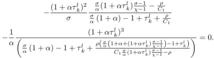
d a but is easier to manipulate algebraically so I will use it. We have: d(log[(1 )W ]) (1 )d a = @(log[(1 )W ]) (1 )@ a + d ~L d a @(log[(1 )W ]) (1 )@ ~L . (32) In Appendix 3 I also deduce the expression for log[(11 )W ], from which I can derive the following:
@(log[(1 )W ]) (1 )@ ~L = (1 ) 1 hhh0200 + 1 1 C1 h0L~ h h0 h a C1 ( 1)h h0 L +~ a , (33) @(log[(1 )W ]) (1 )@ a = 1 1 1 C1 ( 1)h h0 L +~ a . (34)
Substitution of 29, 33 and 34 for the corresponding terms in 32 leads to: d(log[(1 )W ]) (1 )d a = C1 h0 h C1L~ + a + 1 (1 ) C1L~ + a 1 + (35) where denotes ( 1)h
h0L~ 1 and stands for (1 ) 1 hh
00
(h0)2 + 1 . Since > 0 (see Appendix 2, the condition 49) and 1 + > 0 (see the proof for positive B0(L) in Proposition 3), we arrive at the following:
Proposition 6 The su¢ cient and necessary condition for an increase in the lump-sum tax rate to be welfare enhancing is:
(1 ) C1 h0 h C1L~ + a ! + 1 ! 0 (36) where ( 1)h h0L~ 1 and (1 ) 1 hh 00 (h0)2 + 1.
If a value for aexists such that for this value 36 holds as an equality, while
it holds strictly for lower tax rates, 36 gives us an implicit expression for the optimal tax rate a, given the tax program. In the next section I will show that
for speci…cations of tastes and technology parameters often used in calibration exercises it is possible for the tax program to induce Pareto improvements as well as promote growth. The example I o¤er is useful to o¤er an intuition on the mechanism at work in producing the result.
4.4
Are wasted lump-sum taxes good for reasonable
pa-rameter values?
I consider here the following class of functions for the disutility of labor: h(H) = (1 H)1 (37) where > 1 if > 1 or < 1 < + if 0 < < 1.
First we notice that we can now obtain an explicit solution for the equilibrium level of activity. With B( ~L) = 0 and by noting 20 we have:
~ L = 1 1C1+ a C1 + 12+ 1 . (38)
By 24 and again noting 20 we obtain the BGP growth rate:
= 1 1 1C1 1 + 1 + 2 1 + a + 2 1 + 1 . (39)
By using 38 and 39, the e¤ects of lump-sum taxes on BGP labor supply and growth are therefore the following:
d ~L d a = C1 + 12+ 1 and d d a = + 21 1 + 1 .
Both dd ~La and dda are in sign the same with the term + 12+ 1 . This term is positive given the conditions of parameter and in the disutility speci…cation 37: with > 1 the positiveness of this term is easy to be found; with 0 < < 1, we can transform this term into + 11 1 (1 ), whereby since < 1 < + we have 1 > 1 thus this term is also positive.
The welfare level can be written as:
W = ( N (0)) 1 1 1 1 C1 1 1 ~ L 2 C1 1 1 1 L~ L +~ a .
For simplicity in the numerical calculation I normalize the value of ( N (0))1
to 1 by choosing suitable value for N (0) given the value of and .5
5The value of is got from the value of C
1by normalizing A
1
1 to 1 while C1equals r
~ L
Proposition 6 implies that a positive welfare e¤ect requires: 1 1( + 2) 2 41 1 1 ~ L 1 L~ ! + a C1 1 L~ 3 5 0. (40)
Now I try to check whether 40 can hold in reasonable parametrizations of the model. I am completely aware that this model is not rich enough in number of variables, not to mention their dynamics, to …t the data well. Models that are rich enough to …t well become complex and di¢ cult to interpret. The aim of my exercise is not realism but the understanding of mechanisms of action of policy not noticed before in the literature. My choices follow related studies of numerical R&D models (e.g. Jones and Williams (2000), Strulik (2007) and Zeng and Zhang (2007)).
A range of values for labor supply are used in calibration exercises. For example Jones et al. (2005) use ~L = 0:17 while a value of 0.3 is often adopted. In 2005 the average US worker used 21% (24%) of her (his) time endowment to work.6 I choose as benchmark value 0.23 and as range for sensitivity analysis
0.17-0.3.
Coming to 1= , which is the monopoly markup in my model, I choose for it the range (1.1, 1.37) and take 1.2 as the benchmark, corresponding to the range of estimated markups of 1.05-1.4 indicated in Jones and William (2000), while Strulik (2007) …xes it at 1.2.7 Coming to the long-run growth rate, Kenc (2004) chooses 1.5 percent, Strulik (2007) uses 1.75 percent, and Mankiw and Weinzierl (2006) select 2 percent. Therefore I set 1.75 percent as benchmark value and as range for sensitivity analysis 1.5 percent -2 percent. Again following Jones and Williams, the benchmark value for the steady-state interest rate is set to 7.0 percent, which represents the average real return on the stock market over the last century and let it vary between 4.0 percent and 10.0 percent.
is the risk aversion parameter and in the constant relative risk aversion (CRRA) preference as in my model equals the reciprocal of intertemporal elas-ticity of substitution (IES) in consumption. The value of can be tracked either in the literature of estimates of the relative risk aversion (RRA) or in the litera-ture of estimates of the IES. There is considerable debate about the magnitude of the IES. Hall (1988) and Campbell (1999) estimate its value to be well below 1. Other studies that estimate the IES to be smaller than unit include Blundell, Meghir and Neves (1993) (0.5), Attanasio and Weber (1995) (0.6-0.7), Ogaki
6Source: The US Bureau of Labour Statistics, Current Population Survey, March 2005.
For further discussion see chap.2, Borjas(2008).
7Jones and Williams note that in Romer (1990) the monopoly markup is equal to the
inverse of the capital share 1= : Empirically, this implies a gross markup (the ratio of price to marginal cost) of approximately 3, sharply exceeding empirical estimates of 1.05 to 1.4. In our model the capital share is =(1 + ), so the trade o¤ between matching income shares and matching mark-ups is less severe. Taking the data from the IMF’s World Economic Outlook (April 2007) and the European Commission’s Employment in Europe (2007), in the US capital share of income is 39.7% (2005), in EU-15 it is 42.2% (2006) (among which the highest is in Spain, at 45.5%). With markup 1:2, =(1 + ) = 0:4545, with mark-up 1.37 it is
and Reinhart (1998) (0.27-0.766), Vissing-Jorgensen (2002) (0.3-1), Ziliak and Kniesner (2005) (0.7-1), and Engelhardt and Kumar (2009) (with point esti-mate at 0.74 and a 95% con…dence interval of 0.37-1.21). Hansen and Singleton (1982), Attanasio and Weber (1989), Vissing-Jorgensen and Attanasio (2003) estimate the IES to be well in excess of 1. More recently, Hansen, Heaton, and Li (2008) consider a long-run risk model speci…cation where the IES is pinned at 1, while Bansal and Yaron (2004) and Bansal (2007) estimate the IES over 1. However, it is worth noting that those studies with estimates of IES bigger than unit often employ preferences that allow for a separation be-tween the IES and risk aversion (for example Vissing-Jorgensen and Attanasio (2003), Bansal and Yaron (2004) and Bansal (2007)). The RRA in these papers is not generally equal to the reciprocal of the IES and still has values over unit (Vissing-Jorgensen and Attanasio (2003) …nd the lowest value for RRA is 5, and Bansal (2007) sets RRA from 7.5-10). Meanwhile, literature of estimating RRA usually reveals over-unit RRA. Mehra and Prescott (1985) argue that a reasonable upper bound for risk aversion is around 10. Barsky et al. (1997) …nd that the risk aversion of those who hold stocks is around 4.2. Halek and Eisen-hauer (2001), using data from life insurance purchases, estimate risk aversion around 3.75. Tödter (2008) get a point estimate close to 3.5. More relevant to our model, Chetty (2006) discusses two natural measures of risk aversion when hours of work are also included into the preferences. In one, hours are held constant; in the other, hours adjust when the random state becomes known. He notes that risk aversion is always greater by the …rst measure than by the second, …nds a mean estimate of the coe¢ cient of RRA almost equal to 1 and then shows that generating a coe¢ cient of RRA bigger than 2 requires that wage increases cause sharper labor supply reductions. Therefore, the value of in my model is over unit. Considering both literatures, I take a range of from 1.1 to 3 and following Hall (2009) set the benchmark value 2 for it.
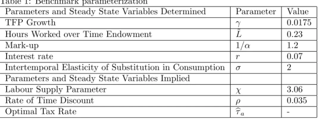
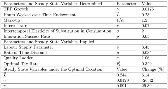
In table 1 I report the benchmark parameterization. The 5-tuplenr; ; ~L; ; o implies values for (through 24) and for (through 38 when a = 0 and
C1= r= ~L through 20).
Table 1: Benchmark parameterization
Parameters and Steady State Variables Determined Parameter Value
TFP Growth 0.0175
Hours Worked over Time Endowment L~ 0.23
Mark-up 1= 1.2
Interest rate r 0.07
Intertemporal Elasticity of Substitution in Consumption 2 Parameters and Steady State Variables Implied
Labour Supply Parameter 3.06 Rate of Time Discount 0.035 Optimal Tax Rate ba
therefore the optimal tax policy in this parametrization should be no tax at all. However, sensitivity test gives out reasonable parametrization under which the wasted lump-sum taxation can be welfare increasing, i.e., dW=d aj a=0 is positive. These welfare-improving results are stated in Table 2.
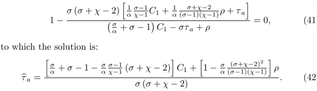
The optimal tax rate ba is obtained by plugging in 40 the expression for ~L
given by 38 and equating it to zero:
1
( + 2)h1 11C1+ 1( +1)( 21) + a
i
+ 1 C1 a+
= 0, (41)
to which the solution is:
ba= h + 1 11( + 2)iC1+ h 1 (( +1)( 2)21)i ( + 2) . (42) The root 42 gives us the optimal value of the lump-sum tax, for each …ve-tuple of the parameters f ; ; ; ; C1g, of which as mentioned above the …rst two
are determined, the other implied. For example, with =1.1 and the other parameters the same as their benchmark value (i.e., the third row in Table 2), it is then calculated that the lump-sum tax rate associated with maximum utility is 8.26%, under which the social welfare increases from -245.31 before tax to -242.92 after tax, hence improved by 0.97%.
Table 2: Alternative parameterizations
=1.1 dW=d aj a=0 d =d aj a=0 ba W=jW j (%) =0.015 1.20 0.054 >0 >0 0.074 0.74 =0.0175 1.21 0.051 >0 >0 0.083 0.97 =0.02 1.21 0.048 >0 >0 0.091 1.26 ~ L=0.17 1.30 0.051 >0 >0 0.133 2.27 ~ L=0.3 1.14 0.051 >0 >0 0.039 0.22 1= =1.1 1.20 0.051 >0 >0 0.083 1.12 1= =1.37 1.22 0.051 >0 >0 0.082 0.77 r=0.04 1.23 0.021 >0 >0 0.072 3.29 r=0.10 1.20 0.081 >0 >0 0.093 0.54 So we see that for a wide region of the reasonable parameters space, a lump-sum tax whose proceeds are disposed will increase growth as well as welfare. This is sensitive to the value of parameter : the welfare-enhancing e¤ect of the wasted lump-sum taxes is made more di¢ cult if is higher.
In order to check that the parameter values for consistent with welfare im-proving lump-sum taxation are reasonable, I calculate the corresponding com-pensated elasticity of labor supply (or, the Frisch elasticity of labor supply, which is obtained by keeping constant the shadow value of wealth) and I com-pare the results with the available estimates. With the speci…cation of the utility
function 37, the Frisch elasticity of labor supply in the BGP is given by (see Appendix 4) 1 + 1 1 1 L~ ~ L , (43)
so it is decreasing in and increasing in . The values of the Frisch elasticity of labor supply consistent with optimal taxation are located between 0.98 and 1.50.8 These values are consistent with the estimates of the Frisch elasticity
found in the literature, which range from 0.5 to 3 or even higher to 3.8 (see, for example, Imai and Keane (2004), Domeij and Flodén (2006) and Prescott (2006)).
5
Economic intuition
After the numerical calculation it is worth noticing that though the growth rate will be largely increased,9 the magnitude of possible welfare gains is not that
large. It is because the lump-sum taxation, whose revenues are wasted, will reduce leisure and instantaneous consumption according to the income e¤ect. The drop in the instantaneous utility should be compensated by a signi…cant increase in the growth rate so as to achieve welfare improvement. That is, the welfare-enhancing e¤ect of the wasted lump-sum taxes can happen should the dynamic gain overwhelm the static loss.
In the present section I …rst explain why the BGP growth rate is increased with the lump-sum taxes whose revenue is thrown to ocean. Then I analyse the two externalities that contribute to the welfare e¤ect, and I also study the role of the parameters , and in in‡uencing the externalities.
1. E¤ect on growth
On …rst impact, the wasted lump-sum taxes reduce the consumers’dispos-able income without changing the opportunity cost of leisure. Since the sub-stitution e¤ect is zero, the income e¤ect on leisure will cause labor supply to increase. Further, the increased labor supply induces a higher demand for the intermediate goods. This in turn induces a higher demand for investment in R&D so the interest rate will rise. Since the BGP growth rate is a monotoni-cally increasing function of the interest rate, it also increases.
2. Two spillovers
There are two spillovers in the economy. Firstly, increased labor supply causes a positive spillover as it increases the value of patents. The worker considers only the increase in labor income w but output increases by w1
1+ where 1+1 is the income share of labor. The di¤erence is a spillover. Notice the size of this spillover is positively related with the value of . This helps
8The values of the Frisch elasticity of labor supply associated with the before-tax parameter
spaces are mainly located between 2 and 3, with 2.06 the lowest and 3.83 the highest. Only in one case the Frisch elasticity is over 3: with =1.1 and ~L =0.17 (i.e., the …fth row in Table 2).
us to understand why the program which increases equilibrium employment is particularly bene…cial when is high. This spillover occurs because the price of intermediate goods is greater than their marginal cost so increased demand for an intermediate good has a …rst order bene…t for its inventor. Secondly, the introduction of a new intermediate good causes increased welfare because it causes increased wages. The inventor only considers the part of the contribution to production that goes to capital (here income on patents). So the e¤ect of an invention on the present discounted value of income is the cost of inventing divided by the income share of capital, that is
1+ . When the return to capital is increased after the introduction of lump-sum taxes, the pace of invention of new patents will be accelerated. So this is also positive spillover.
3. Level e¤ect
With the extraction of lump-sum taxes, the instantaneous consumption de-creases according to the negative income e¤ect. Considered that the leisure is also reduced, this causes a loss to the static level of welfare. Therefore, though the two positive spillovers can result in higher equilibrium growth rate, their e¤ects are counteracted by the loss of the static level of welfare. The sign of overall welfare e¤ect of the tax program is thus determined by the relatively stronger one given the tradeo¤ between growth and level.
4. Factors in‡uencing the welfare e¤ect
Two things in‡uence the magnitudes of the spillovers. One is the income share of labor: if it is small the …rst spillover is large and the second is small. However, since the two spillovers are both positive, the value of does not alter much the magnitude of their joint e¤ect on welfare. This can be seen from the comparison between row 7 and 8 in table 2 that the optimal rates of the wasted lump-sum taxes do not di¤er from each other much. The other is the e¤ect of the policy on labor supply, for which the elasticity of labor supply plays an important role. In our speci…cation of the disutility function of labor 37, the elasticity of labor supply is decreasing in the parameter and ~L but increasing in the parameter (see 43). A smaller or ~L means higher elasticity of labor supply so a cut in disposable income will cause labor supply to increase much. To see the in‡uence of parameter , since in our numerical calculation is obtained by the implied value from the function between and the other parameters fr; ; ~L; ; g, we should compare the results under di¤erent values of which are generated with only one determining parameter free and the others …xed. Therefore, we can refer to row 7 and 8 in table 2, where fr; ; ~L; g are the same with only varying, that the bigger is , the lower is the optimal rate of tax and the smaller is the improvement of welfare. As for the a¤ect of ~L, we can …nd from row 5 and 6 in table 2 (where the free parameters fr; ; ; g are the same) that the smaller is the before-tax labor supply ~L, the higher is the optimal tax rate as well as the welfare improvement.
A bigger also means smaller intertemporal substitution elasticity of con-sumption, or that consumers weigh more the current consumption (lower) than the future (higher) ones. So, when the instantaneous consumption is decreased with the wasted lump-sum taxes, this reduction is given more weight than the
future gain. This can explain why with big we can only have welfare reduced by the tax: big means small IES in consumption, therefore to keep the same utility level the reduction in instantaneous consumption should be compensated by large increase in future consumption, which renders it di¢ cult to achieve the welfare improvement.
The tradeo¤ between the opposing growth and level e¤ect of the tax program also depends on the subjective discount rate of the representative household. With smaller the tax program can be more easily to enhance welfare: smaller means that the discounted value of the future consumption, growing at a given growth rate, will be bigger so that it can more easily compensate for the loss in instantaneous consumption. In table 2, bigger or lower r implies smaller , and associated with it we can see the bigger potential of the tax to improve welfare.
Appendices
Appendix 1
By 18 and 20 we can get the following relationship between labor income and capital income:
wL = r N. (44) Using the factor exhaustion condition that the wage bill plus total interest pay-ments is equal to GNP, that is Y xN = wL + r N , substituting for C using equation 7 and noting 44, we can write 23 as:
_ N
N = r 1
1 ( 1)h(L)
h0(L)L 1 a. (45)
Substituting 25 for CC_ in 8 we get: " _ N N + (h 0=h h00=h0) _L # +h0 hL =_ r. (46) Finally if we substitute in 46 the expression for NN_ given by 45 we obtain 26 in the text.
Appendix 2
Transversality condition 9 requires < r. In an initially taxless economy, 45 gives in equilibrium
= r 1 1 ( 1)h(L) h0(L)L 1
so < r leads to
( 1)h(L)
h0(L)L > 1. (47)
In addition, in a growing economy the investment should be positive, there-fore in an initially taxless economy there should be
C < Y xN , for which by using 7, 16, 17 and 18 we get
( 1)h(L)
h0(L)L < 1 + . (48)
Combining condition 47 and 48 we have 1 < ( 1)h(L)
h0(L)L < 1 + . (49)
Appendix 3
By solving the integral in 31 we obtain:
W = 1 1
C(0)1 h( ~L)
(1 ). (50) By using 7, 20 and 44 we can write:
C(0) = N (0)( 1)h( ~L) h0( ~L)
C1
where N (0) is the initial stock of patents. Using 24 we have: (1 ) = r ,
while by using 45 to get an expression for , we obtain: r = r ( 1)h( ~L) h0( ~L) ~L 1 ! + a = C1L~ ( 1)h( ~L) h0( ~L) ~L 1 ! + a.
We can thus rewrite 50 as: W = ( N (0)) 1 1 1 h0( ~L) C1 1 h( ~L)2 C1L~ ( 1)h( ~L) h0( ~L) ~L 1 + a .
Thus we have the increasing monotonically transformation of W :
log[(1 )W ] 1 = log( N (0)) + log 1 h0( ~L) + log C1 +2 1 log(h( ~L)) 1 1 log C1L~ ( 1)h( ~L) h0( ~L) ~L 1 ! + a ! .
Appendix 4
To calculate the Frisch elasticity of labor supply we have that one optimality condition of the household is:
( 1)w
h0(H) h(H)
1 = . (51)
Since the Frisch elasticity of labor supply is the measure under constant mar-ginal utility of wealth (here it is ), we can take the total derivative with respect to H and w for equation 51, keeping …xed and derive the following:
dH dw j =
h(H)h0(H)
w ((1 )h0(H)2+ h(H)h00(H)). (52)
Therefore the Frisch elasticity of labor supply eF is
eF = dH dw j w H = h(H)h0(H) H ((1 )h0(H)2+ h(H)h00(H)). (53)
With the speci…cation of labor-disutility function in our model, the Frisch elasticity of labor supply is thus
eF = 1 +
1 11 H
H . (54) In the BGP the Frisch elasticity of labor supply is exactly that in the text.
Chapter II. Lump-sum taxes in a
creative destruction model
6
The model
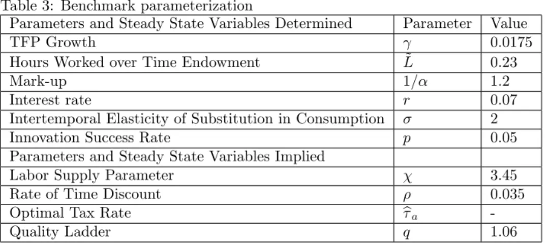
The last chapter modeled technological progress as an increase in the number of types of products, N . In this chapter, we allow for improvements in the quality or productivity of each type. This approach has come to be known as the Schumpeterian approach to endogenous growth. An important aspect of the Schumpeterian model is that, when a product or technique is improved, the new good or method tends to displace the old one. Thus it is natural to model di¤erent quality grades for a good of a given type as close substitutes. We make the extreme assumption that the di¤erent qualities of a particular type of in-termediate input are perfect substitutes; hence, the discovery of a higher grade turns out to drive out the lower grades completely. For this reason, success-ful researchers along the quality dimension tend to eliminate or "destroy" the monopoly rentals of their predecessors, a process labeled as "creative destruc-tion" by Schumpeter (1934) and Aghion and Howitt (1992). On the normative side, the process of creative destruction implies a "business-stealing" e¤ect.
With no assumption on either cost advantage or complete property right, a monopolist always has lower incentives to undertake innovation than a compet-itive …rm. This result, which was …rst pointed out in Arrow’s (1962) seminal paper, is referred to as the replacement e¤ect. The terminology re‡ects the intuition for the result; the monopolist has lower incentives to undertake inno-vation than the …rm in a competitive industry because with its innoinno-vation will replace its own already existing pro…ts. In contrast, a competitive …rm would be making zero pro…ts and thus had no pro…ts to replace. An immediate and perhaps more useful corollary of this proposition is the following: An entrant will have stronger incentives to undertake an innovation than an incumbent mo-nopolist. The potential entrant is making zero pro…ts without the innovation. The replacement e¤ect and this corollary imply that in many models entrants have stronger incentives to invest in R&D than incumbents. Acemoglu (2009) supplies a good survey of the innovation by entrant, which directly leads to the so-called business-stealing e¤ect.
The economy in the present chapter is the same as in the previous chap-ter except that the R&D activity contributes to new patents so as a series of increasing quality of intermediate goods. That is, there is obsolescence of any type of intermediate goods when a new patent is invented successfully. The household sector and the government sector are the same as those in the variety expansion model so hereby I avoid repeat. In this section I focus on the model for …rms.
6.1
Final good sector
Following again Spence (1976) and Dixit-Stiglitz (1977) the production function of …rm i in the …nal good sector is given by:
Y (i) = AL(i)1 Z N
0
~
x(i; j) di (55)
where A is a positive technologic parameter, is the ratio of intermediate input and 0 < < 1, N is the dimension of the varieties of intermediate goods in the economy and is assumed …xed in this model, Y (i) is the amount produced and L(i) is labor used by …rm i and ~x(i; j) is the quality-adjusted quantity this …rm uses of the intermediate good indexed by j, and is de…ned as
~
x(i; j) = qkjx(i; j) (56) where x(i; j) is the physical input of the intermediate good j by …rm i, q is the unit of rung of the quality ladder and q > 1 as well as q 1,10 kj is the
improvements in quality that have occurred in intermediate good sector j. For tractability both i and j are treated as continuous variables. The …nal good production sector is competitive and I assume a continuum of length one of identical …rms. I can then suppress the index i to avoid notational clutter.
The numeraire in the economy is one unit of …nal output and the price of any …nal good is standardised to 1. Firms maximize pro…ts given by
Y wL Z N
0
P (j)x(j)dj
where w is the wage rate and P (j) is the price of the intermediate good j. By pro…t maximization we have:
x(j) = A q kj P (j) 1 1 L (57) and w = (1 )Y L. (58)
6.2
Intermediate good sector
6.2.1
Production
Suppose the production of intermediate goods utilizes only …nal output and by choosing the unit of intermediate goods I can set the marginal cost to 1. The inventor of the jth intermediate good chooses P (j) to maximize pro…ts
(P (j) 1)x(j) where x(j) is given by 57, so for each j:
P (j) = P = 1 (59) and
x(j) = LA11 12 q kj=(1 ). (60) I de…ne the aggregate quality index
Q Z N
j=1
q kj=(1 )dj. (61)
Summing over j the both sides of equation 60 we get the total output of inter-mediate goods X = Z N j=1 x(j)dj = QLA11 2 1 . (62)
Using 60 and noticing 61, we get the …nal goods output Y = QLA11
2
1 . (63)
From 62 and 63 we get the relation
Substituting 63 for Y into equation 58, the wage rate is now w = Q(1 )A11 2 1 . (65) I de…ne (1 )LA11 1+ 1 . (66)
By using 59 and 60, the pro…t of the intermediate good j producer is then (kj) = q kj=(1 ). (67)
So the total pro…t of the intermediate good sector is
= Z N
j=1
(kj)dj = Q. (68)
Using 63, 66 and 68 we get the relation
= (1 )Y . (69)
6.2.2
R&D Activity
Let p(kj) denote the probability per unit of time of a successful innovation in
the jthintermediate good sector when the top-of-the-line quality is k
j. In other
words p(kj) is the probability per unit of time that an outside researcher will
raise the quality of intermediate good j from kj to kj+ 1. Assume that the
probability of the incumbent losing his monopoly position is generated from a Poisson process.
I assume that p(kj) depends positively on R&D e¤ort z(kj), which is the
aggregate ‡ow of resources expended by potential innovators in sector j when the highest rung available is kj; and that p(kj) also depends negatively on (kj),
which captures the increasing di¢ culty of innovation with the increasing kjand
is represented by
(kj) =
1
q (kj+1)=(1 ) (70)
where > 0 is a parameter that represents the cost of doing research. Ad-ditionally, I assume that the distribution of the expenditure across researchers does not have any in‡uence on p(kj). Thus, the probability of research success
is endogenized as
p(kj) = z(kj) (kj). (71)
As what has described, p(kj) is increasing in z(kj) and decreasing in (kj).
If I let tkj be the moment when the kjquality improvement is made and tkj+1 the time of the next improvement by a competitor, ‡ow of pro…t (kj) applies
only from time tkj to tkj+1. Let T (kj) denote the duration of the monopoly for the inventor of rung kj, that is, T (kj) tkj+1 tkj.
Denote by v(kj) the present value of all the pro…ts that the inventor of rung kj evaluated at time tkj: v(kj) = Z tkj +1 tkj (kj)e r(s;tkj)(s tkj)ds (72) where r(s; tkj) 1 s tkj Z s tkj r(!)d!
is the average interest rate between times tkj and s. In a balanced growth equilibrium, the interest rate should be a constant r. Hence in equilibrium, the present value 72 can be simpli…ed as
v(kj) =
1
r (kj)[1 exp( r T (kj)]. (73) Since T (kj) is a random variable subject to the Poisson process with the
arrival rate p(kj), by noticing the equation 67 for substituting for (kj) in
equation 73, the expected present value is in fact E[v(kj)] =
r + p(kj)
q kj=(1 ). (74)
I assume that potential innovators care only about the expected present value E[v(kj+ 1)] and not about the randomness of the return. Free entry is
allowed in the R&D activity. Thus the net expected return per unit of time in the R&D investment must be zero. That is, we have the free entry condition
p(kj)E[v(kj+ 1)] z(kj) = 0. (75)
By substituting for p(kj) from equation 70 and 71, and using 74 for E[v(kj+
1)], for any positive expenditure z(kj), equation 75 becomes
r + p(kj+ 1) = . (76)
Therefore, equation 76 means that the probability of research success per unit of time is the same in each sector, independent of the quality-ladder position, and is given by
p = r. (77)
By using equation 71 for z(kj), and using 70 for (kj) as well as 77 for p,
the amount of total resources devoted to R&D is Z =
Z N j=1
Substituting for p from equation 77 into equation 74, we get the aggregated market value of …rms V = Z N j=1 E[v(kj)]dj = Q. (79)
7
Market equilibrium
To obtain total value added, the total of intermediate goods used X is subtracted from …nal production Y . Again, all investment in the model is the investment in research and development of more advanced intermediate goods Z. The economy-wide resource constraint is therefore given by
Y X = C + Z + G. (80) Notice that in equilibrium the households’…nancial wealth equals the total value of existing …rms in the economy, i.e. F = V . Thus, since G = aF (see 21), the
social budget constraint 80 can be rewritten as
Z = Y X C aV . (81)
We are now ready for the following:
De…nition 7 In a competitive equilibrium individual and aggregate variables are the same and prices and quantities are consistent with the (private) ef-…ciency conditions for the households 6, 7, 8 and 9, the pro…t maximization conditions for …rms in the …nal goods sector, 57 and 58 (or 65), and for …rms in the intermediate goods sector, 59 (or 60) and 77, with the government bud-get constraint 21 and with the market clearing conditions for labor H = L, for wealth F = V , and for the …nal good, 80.
I consider only the balanced growth path (hence BGP) of the model: labor supply L, interest rate r, research success probability p are constant while the other variables, including consumption C, aggregate quality index of the patents Q, wealth (or capital) F , and R&D expenditure Z are at the same constant growth rate.
8 implies that along a BGP with L constant consumption grows as: _
C C =
r
. (82)
We need track down the technic growth rateQQ_. Since in each intermediate good sector, the quality does not change if no innovation occurs but rises up for one rung in the case of research success, and since the probability per unit of time of a success p is the same for all sectors, the expected change rate in Q per unit of time is thus given by
E( Q) Q = 1 Q Z N j=1 p[q (kj+1)=(1 ) q kj=(1 )]dj = p q1 1 . (83)
Suppose the variety of the intermediate goods, N , is large enough to treat Q as di¤erentiable, by the law of large numbers, the average growth rate of Q measured over any …nite interval of time QQ_ will be non stochastic and equal to
E( Q)
Q . Substituting for p from 77 into 83, we get the growth rate of Q:
_ Q
Q = r q
1 1 . (84)
Proposition 8 If the economy follows a balanced growth path (hence BGP) variables grow at a constant rate, and in particular employment is constant at a value ~L. Along this path, rate of growth of capital and consumption, , is then given by
=
q1 1 ( ~L) 1 + q1 1
. (85)
Proof. When labor supply is constant at ~L, the wage w is proportional to the aggregate quality index Q by 65, so w and Q grow at the same rate. And 7 implies that consumption and the wage must grow at the same rate so we have:
_ C C = _ Q Q . (86)
By using 82, 84 and 86, we can solve out the BGP growth rate as 85, and interest rate r as follows:
r = +
( ~L)
q1 1
1 + q1 1 . (87) Substitution for r from equation 87 into 77 helps to get the endogenous inno-vation success rate p:
p =
( ~L)
1 + q1 1 . (88) Equations 85, 87 and 88 show that with q1 > 1 and an increasing function of L (see 66), the BGP , r and p are all increasing in L.
In Appendix 5 I show how to deduce from the competitive equilibrium con-ditions described above the following di¤erential equation of labor, which is the fundamental dynamic equation of the model:
_ L = + ( 1)r + 1 + (1h0L)h a h00 h0 + (1 )h 0 h B(L) A(L). (89) Hereby the denominator of the fraction on the right-hand side A(L) is always strictly positive for all values of L for the same reason as stated in the counter-part in Chapter 1. So the equation is de…ned for all values of L beween 0 and 1.