REALISTIC UTILITY VERSUS GAME UTILITY: A PROPOSAL FOR DEALING WITH THE SPREAD OF UNCERTAIN PROSPECTS B.V. Frosini
1. INTRODUCTION. CONCEPTS AND MEASURES OF UTILITY
This article is a contribution towards modelling the preference behaviour of individuals, along the lines that in recent decades have abandoned – or general-ized – the classical Expected Utility (EU) approach of von Neumann-Morgen- stern-Savage (N-M-S for short). The viewpoint accepted in this paper starts from the recognition – in agreement with many important scholars – that the utility of certain or sure prospects is relative to the prospects themselves, and cannot obey probabilistic constraints, and also that the attitude toward risk taking is separated from the strength of preference concerning certain outcomes (see e.g. Bernoulli, 1738/1954; Allais, 1953, 1988; Dyer and Sarin, 1982; Hansson, 1988; Wakker, 1994). As a consequence, in evaluating and predicting risk behaviours, one must consider a realistic utility function, and the evaluation of a risky prospect must be based – in principle – on the whole probability distribution of the prospect (Al-lais, 1953, pp. 504, 509).
Along these lines, a utility function ug for the game (or wager, or random variable
offered to the subject) can be assumed, which allows to assess the importance or eagerness of the game on the utility scale. In order to achieve a simple and tracta-ble operational device, beside the mean of utilities, as in the N-M-S approach of Expected Utility, a measure of dispersion is also introduced, following the sugges-tion of Allais: “l’erreur fondamentale de toute l’école américaine, c’est de négliger indirectement et inconsciemment, la dispersion des valeurs psychologiques” (1953, p. 544). The operational approach consists, quite simply, that the evalua-tion funcevalua-tion (of an uncertain prospect) raises with the mean of utilities, and – for a risk averse subject – diminishes with the mean absolute deviation (MA) of utilities (formula (5) of this paper); this measure of dispersion is conveniently multiplied by a parameter λ, whose sign and magnitude depend on the contingent attitude of the subject in evaluating a given prospect, starting from a given asset position; it will be seen that such a parameter must be constrained between limits 0 and 0.5 for a risk averse subject, in order to comply with the dominance requisite. This is admittedly a simplistic and first approximation approach – however much less
simplistic and much more realistic than the Expected Utility approach. A more refined, but also more demanding technique, aiming all the same at disentangling the two main contributions to the explanation of risk behaviour, has been studied by Wakker (1994), in the contest of rank-dependent utility models.
This article follows a previous proposal by Frosini (1997), and is itself an abridged version of an extended paper (Frosini, 2010), available in the pre-print series of the Department of Statistics of the Catholic University of Milan. The a-vailability of both papers makes it easy to concentrate the formal developments to new issues, while referring to one or other of these papers for specific topics here only mentioned.
Let h1, ..., hn be certain (or sure) prospects, and p = (p1, ..., pn) a probability
dis-tribution over them (pi ≥ 0 i; pi = 1); a general finite prospect can be written d = [h1,p1; ...; hn,pn]. The above certain prospects can be related to final personal
wealth, or else to changes of the present status quo; different treatments of the two cases will be resumed later on. Each sure prospect hi is endowed with a utility ui = u(hi), formally defined except for an affine transformation; let U = [u(h1), p1; ...; u(hn),pn] = [u1,p1; ...; un,pn] be the rv (= random variable) which matches the
utilities with their respective probabilities. Continuous distributions could be em-ployed as well, with no essential modifications in the sequel. Both classical ap-proaches by Daniel Bernoulli and by von Neumann and Morgenstern define the utility of a risky prospect d as the arithmetic mean, or expectation,
u(d) = E(U) = u = u(hi)pi; (1)
among two or more prospects, one should choose the one which maximizes ex-pected utility (Lindley, 1985, p. 59).
J. Quiggin (1982, 1985, 1993) suggested transformation functions (see Kahne-man and Tversky, 1979) from single probabilities to cumulative probabilities, thus saving most desirable properties of EU (Expected Utility) theory; his approach is usually condensed in the acronym RDEU (= Rank-Dependent Expected Utility). The expected value of EU theory was replaced by an evaluation function (with like appearance)
V(x,p) = u(xi)ki(p) (2)
where
ki(p) = q(
ir1pr) – q(
ir11pr).In other words, the original probabilities pi are changed by means of a probabil-ity-perception function so as to reflect the personal appreciation and risk attitude of
the decision maker through the function q applied to the cumulative probabilities.
A special and common case of prospect is concerned with sums of money; the generic prospect of this kind will be symbolized by d = [x1,p1; ...; xn,pn] (xi xi+1),
being xi a real number, expressing a sum of money (negative, null or positive) in a
If d’ = [x1’,p1’; ...; xn’,pn’ ] is another prospect, such that xi’ ≥ xi, and/or there is a
transfer in probabilities towards larger xi values, then d d’. This property,
objec-tively based, is usually named monotonicity property, or (first) dominance property.
All cases, discrete and continuous, can be included in a definition which refers to the cdf’s (cdf = cumulative distribution function) of the rv’s being compared: if
X1 and X2 are two monetary prospects, with respective cdf’s F1 and F2, X1
domi-nates X2 (X2 X1) (or, equivalently, F1 dominates F2) if F1(x) F2(x) for all x
(Quiggin, 1993, pp. 16, 21-25). The cited “dominance property” is often referred to in the literature as first stochastic dominance (FSD); the fact that X1 dominates X2
is usually symbolized by X1 FSD X2.
Although maintaining the (first) dominance principle as absolutely requisite, other two connected criteria appear also adequate in order to establish a reason-able and interesting partial ordering between probability prospects: the mean-preserving spread (Rothschild and Stiglitz, 1970, pp. 226-230; 1971; Diamond and Stiglitz, 1974), and the mean-preserving monotone spread (Quiggin, 1991; 1993 p. 85). A much wider comment about these and other related criteria is referred to Frosini (2010, pp. 3-12).
2. AN OPERATIVE SPECIFICATION OF THE UTILITY OF THE GAMEug
2.1 The influence of risk attitudes on the utility of uncertain prospects
The definition of a risk neutral behaviour demands a strong, although reason-able, convention, which goes back to Daniel Bernoulli (1738/1954), meaning that
one is indifferent between maintaining a game (a random variable) or accepting the certain value given by its expectation. Such neutral behaviour acts as a water-shed between the common risk averse behaviour (the preference goes to the ex-pectation) and the infrequent risk prone behaviour (maintenance of the game). As one is usually interested in the characterization of risk averse behaviour, this kind of behaviour could be called weak risk aversion (in agreement with Chateauneuf et al., 2005, p. 650; a partially different definition is the one given by Quiggin and
Chambers, 1998, p. 124).
Such final, or external, or revealed behaviour appears as the conjoint result of (at least) two independent factors, the curvature of the (realistic) utility function and the attitude toward risk. The former can be assumed concave for practically all individuals, while it can be assumed reasonably linear for many firms, compa-nies and institutions. The final behaviour obviously depends on the interaction between these two factors: “a DM [decision maker] with diminishing marginal utility on certain wealth may be risk-seeking” (Chateauneuf et al., 2005, p. 650).
As the real attitude toward risk cannot be derived from the utilities of certain prospects, it is expedient to introduce the concept of g-risk attitude (g for game),
which depends on the uncertainty of the game for a subject; concerning risk aver-sion, this concept is practically overlapping with “aversion to mean-preserving increase in risk (MPIR) in the sense of Rothschild and Stiglitz” (Chateauneuf et al.
words “weak” and “strong” are not most suitable for the above characterization: they can be taken as conventional symbols, devoid of proper meaning).
Following Frosini (1997, p. 442), the reference to the expected value of utilities can be advantageously maintained in the model for the case of g-risk neutral
be-haviour, while g-risk averse and g-risk prone behaviours are related to the
diver-gence of the utility of the gamble d = [h1,p1; ...; hn,pn] (uncertain prospect) from the
expectation. The essential feature of this approach consists in assuming a utility
ug(d) which mirrors the individual attitude towards risky prospects, and does not
match – except in special cases – the expectation of utilities. Thus we have the following three specifications:
(a) an individual is g-risk neutral for the prospect d if the utility of the prospect
equals the expected value of utilities, i.e. if ug(d) = u ;
(b) an individual is g-risk averse for the prospect d if its utility is less than the
av-erage utility, i.e., for δ(d) > 0, ug(d) = u – δ(d);
(c) an individual is g-risk prone for the prospect d if its utility is greater than the
average utility, i.e. if, for δ(d) > 0, ug(d) = u + δ(d).
The simplest structure – and corresponding graphical display, see Figure 1 – of this approach, is related to the evaluation of a binary prospect d = [0,1 – p; 1,p]; in
this case the realistic utility u(x) (x = money, according to an appropriate scale),
and the utility for risky prospects ug(p), can both be plotted in a square of side one
(with a different meaning for the abscissas of the two functions). For practically all individuals the realistic utility is a concave function (with decreasing marginal utility), while the utility ug(p) is a convex function for risk averse individuals. The certainty equivalent x = CE(d) of the binary prospect d results from the equation
u(x) = ug(p) x = u-1○ug(p)
and for a general prospect d:
u(x) = ug(d) x = u-1○ug(d). (3)
Note that the certainty equivalent x uttered by an individual is of course
inde-pendent of any theory contrived to explain the relation between x and the risky
prospect d; anyway, the apparent relation displayed by equalizing the expectation p
of d = d(p) = [0,1 – p;1,p] to the N-M-S utility v(x) becomes
u = p = ug-1○u(x) = v(x) (4)
thus showing that the N-M-S utility equals – under the above theory – the com-position ug-1○u. For most people ug is convex, which implies that application of ug-1 to u boosts the concavity of the utility function for sure outcomes.
The above equalities and related comments are exemplified in Figure 1, which is referred to the functions
ug(p) = p(1 + p)/2 (with λ = 0.25 in formula (6)); u(x) = x0.7 x(p) = u–1(p) = [p(1 + p)/2]1/0.7
0 1 0 x p 1 x,p p=v(x) ur(x)=ug(p) ug v u=ur
Figure 1 – Example of relevant functions for binary games in the case of risk averse behaviour. x = monetary outcome, p = probability of success for the game d(p) = [0,1 – p; 1,p], ug(p) = utility of
the game, u(x) = ur(x) = realistic utility of x, v(x) = von Neumann-Morgenstern utility of x (not a
realistic utility).
The parametric specification of ug proposed by Frosini (1997) for the case of
monetary outcomes x1, ..., xn, mainly in view of its simplicity, is the following:
ug(d) = u(xi)pi - λ |u(xi) – u |pi = u – λMA(U) (5)
i.e. by subtracting from the expectation u a term proportional the the mean
ab-solute deviation MA of utilities. This criterion is invariant with respect to linear transformations of utilities, meaning that, if U = [u1,p1; ...; un,pn] and V = a + bU,
the following relation holds:
ug(V) = ug(a + bU) = a + bug(U).
2.2 Satisfying the first stochastic dominance
We assume throughout - as a quite natural requirement - the validity of (first) stochastic dominance, namely that the risky prospect d2 is preferred to d1 when
the following inequality takes place between the distribution function F1 of the
random variable d1 = [u1,p1; ...; un,pn] and the distribution function F2 of the
ran-dom variable d2 = [u1,p1’; ...; un,pn’] (ui ≤ ui+1): F2(x) ≤ F1(x) for ∞ < x < ∞
In the case of a binary prospect d(p) = [0,1 – p;1,p], stochastic dominance is
di-splayed by increasing p values. On account of this fact, the range of admissible values is easily established for the case of binary prospects; actually, in this case
ug(d) = f(p) = p – 2 λp(1 – p) 0 ≤ p ≤ 1 (6)
being positive for risk averse individuals, and negative for risk prone individuals.
If we want the criterion ug to be consistent with stochastic dominance, this
con-vex function must be increasing from p = 0 to p = 1, which occurs when 0 < ||
< 0.5; for example, when = 0.75, f(p) = p(1.5p – 0.5) has roots 0 and 1/3, and
is decreasing for 0 < p < 1/6. A conjectured “mean risk aversion” is related to
= ¼, which implies ug(d) = p(1 + p)/2 (0 ≤ p ≤ 1).
This same result for the range of values (|| < 1/2) can be achieved by looking for the admissible values in the general formula (5). Let us start by rewrit-ing the mean absolute deviation MA as follows:
MA = ∑ | ui – u | pi = 2 ( ) i i i u u u u p
= 2 ( ) i i i u u u u p
= 2 i i i u u u p Pu
being P = i i u u p
. As the values ui are in ascending order, and we mayconven-tionally assume that 0 ≤ u1 ≤ ... ≤ un = 1, the difference in (5) takes its minimum,
given u and , when MA is a maximum, which happens when 1 i i i u u u p u P
= E(ui | ui > u ) – uis a maximum. Given 0 ≤ u ≤ 1, max [E(ui | ui > u ) – u ] is clearly attainable
when the only probabilities different from zero are p1 = 1 – u and pn = u ;
there-fore, the maximizing value of MA is 2 u (1 – u ), and the minimum value of ug(d)
is
ug(d) = u – 2 λ u (1 – u ) (7)
which looks like formula (6) – and actually, in this case, u = p; the maximum value allowable for is therefore 0.5.
This same range for values is required in order that the criterion (5) satisfies the First Stochastic Dominance (FSD) in the general case. Let us consider a dis-placement of probability from d1 = [u1,p1; ...; un,pn] to d2 = [u1,p1’; ...; un,pn’] (pi, pi’ ≥
0) such that pi’ = pi for i r,s, pr’ = pr (such that pr ≥ 0), ps’ = ps + , for ur < us. The criterion FSD is satisfied if, in any case, ug(d1) < ug(d2). In any case the
expectation is increased from u to
u ’= , ( ) ( ) ( ) i i r r s s s r i r s u p u p u p u u u
thus complying – as it is well known – with the criterion FSD. For the complete expression ug(d) let us consider three distinct cases, with subcases:
(a) ur < us u ;
(a1) there are no ui’s such that u ui u ’; in this case the new MA’ can be
written MA’ = 2 [ ( )] i i s r i u u u u u u p
, so that ug(d2) ug(d1) = u + (us ur) 2MA’ u + 2MA= (us ur)(1 + 2P ) > 0, which holds in any case when > 1/2.
(a2) There are values ui’s such that u ui u ’= u + (us ur); in this case
MA’ reduces to MA’ = 2 ' ( ') i i i u u u u p
so that the previous difference ug(d2) ug(d1) is increased.
(b) u ur < us;
(b1) there are no ui’s such that u ui u ’; in this case the new MA’ can be
written MA’ = 2 [ ( ) ] i s r i i u u u u u u p
so that ug(d2) ug(d1) = u + (us ur) 2MA’ u + 2MA = (us ur)[1 2(1 P )]which is greater than zero in any case when < 0.5.
(b2) There are values ui’s such that u ui u ’; in this case MA’ is increased to
MA’ = 2 , ' ( ' ) i i i u u u u p
so that ug(d2) ug(d1) = u + (us ur) 2MA’ u + 2MA = (us ur)[1 2 i i u u p
] 2 , ' ( ' ) i i i u u u u u p
.If, in the last summation, ui is replaced by u , the same summation is increased to
(us ur) , ' i i u u u p
so thatug(d2) ug(d1) = (us ur)[1 2 , ' i i u u p
] = (us ur)[1 2(1 P ’)]thus we find anew that such a difference is greater than zero in any case when
< 0.5.
(c) ur < u < us.
This case can be treated by means of two successive displacements of prob-ability , the first from pr to the probability of u (possibly starting from a null
value), and the second from the probability of u to ps, thus by means of
succes-sive applications of the cases (a) and (b). 2.3 Satisfying the independence condition
A property maybe unexpected of criterion (5) is that it satisfies the so-called
inde-pendence condition, which is introduced as an essential property or axiom in the
ortho-dox Expected Utility theory (special case of (7) for = 0); this requisite is satisfied under the same constraint for (|| < 1/2), which ensures the compliance with the dominance property, just demonstrated. Such a condition says that, if prospect
B is preferred to prospect A, a probability mixture of B with any other prospect C
is always preferred to the same kind of mixture between A and C; in symbols:
A B ↔ d = [A,p; C,1 – p] d’ = [B,p; C,1 – p] for any prospect C and 0 < p 1.
A similar condition is called sure-thing principle by Savage (1954) (cf Frosini and Giossi, 1994, par. 5).
Let a, b, c (a < b) be the utilities of the corresponding prospects A, B, C.With reference to the generic binary prospect [A,p; B,1 – p], the following expressions for the mean utility u and the mean absolute deviation MA hold:
u = ap + b(1 – p)
MA(U) = (ap + b(1 – p) – a)p + (b – ap – b(1 – p))(1 – p) = 2p(1 – p)(b – a). Now, let the following cases be examined: (I) a < b c; (II) a c b; (III)
c a < b.
For case (I)
ug(d) = ap + c(1 – p) - 2λp(1 – p)(c – a) ug(d’) = bp + c(1 – p) - 2λp(1 – p)(c – b)
so that ug(d’) > ug(d) when
p(b – a)(1 + 2λ(1 – p)) > 0. (8)
When λ > 0 in (5), namely for a risk averse subject, this condition is naturally satisfied: the mixture of C with A ensures a lower expected utility and a larger
di-spersion than the mixture with B; both comparisons yield a larger utility ug(d’). For
a risk prone subject, i.e. when λ < 0, inequality (8) is satisfied when | λ | < 1/ (2(1 – p)), thus | λ | < 1/2 is the proper condition.
For case (II), ug(d’) > ug(d) when
p(b – a) – 2λp(1 – p)(a + b – 2c) > 0. (9)
If (a + b)/2 c b, it is immediately recognized that the second term of the al-gebraic sum (9) is positive or null for every λ > 0, so that the > sign is satisfied. When, to the contrary, λ < 0, the condition to be satisfied is | λ | < 1/2. If a c (a + b)/2, the most unfavourable situation for (9) to hold for λ > 0, is that c = a, in which case the sign > holds for λ < 1/2. Instead, when λ < 0 the most unfa-vourable situation is for c = (a + b)/2, hence the left hand side of (9) reduces to
p(b – a) > 0 for every negative λ.
For case (III), ug(d’) > ug(d) when
p(b – a)(1 - 2λ(1 – p)) > 0. (10)
For λ > 0 we find anew the condition λ < 1/2. For λ < 0 no further constraint on λ arises.
2.4 The shapes of indifference curves
About the shapes of indifference curves inside the Marshak-Machina triangle, the interested reader is referred to Frosini (2010, par. 5.4).
2.5 Why not to use the standard deviation of utilities
Another natural application of the above criterion could be equating δ(u(x)) to a value proportional to the standard deviation SD of the distribution U of utilities
ug*(d) = uipi - [(ui - u )2pi]1/2 = u - SD(U). (11)
Marshak (1950, p. 120, Note 10) reports that “As a measure of riskiness the standard deviation was suggested by I. Fisher as early as 1906”. However, if we want not to give up the stochastic dominance requirement, the criterion ug*
pre-sents serious shortcomings. In fact, if we choose for convenience – as usual – va-lues u(xi) = ui 0, the maximum reduction of u in (11) occurs in cases of
maxi-mum dispersion of the values ui around a fixed mean u ; just as for the variability
measure MA, if 0 ≤ ui ≤ 1 for i = 1. ..., n, maximum dispersion is achieved when
the distribution is binary, i.e. when U = [0,1 – u ; 1, u ], with mean u (cf. Fro- sini, 1984, p. 392); therefore the minimum ug*(d) is
ug*(d) = u – λ [ u (1 – u )]1/2 (12)
Problems arise for u in a neighbourhood of zero. In fact, as we approach zero from the right, the derivative of ( u ) = [ u (1 – u )]1/2 tends to +∞, whereas the
derivative of u is 1; practically, for 0 < u < λ2/(1 + λ2) the negative term (for λ > 0) in (12) overcomes u , thus there is an interval for u – for every λ > 0 – in
which ug*( u ) decreases as u increases (contrary to the requirement of
domi-nance).
2.6 Other similar proposals
We have seen above the validity of proposal (5) for 0 ≤ λ ≤ 0.5 in case of risk averse subjects, and the rejection of (11) for any λ ≥ 0, on the basis of the fun-damental criterion of stochastic dominance. A class of similar criteria, for the rv
X = (x1, p1; ...; xn, pn), has been envisaged by Quiggin and Chambers (1998, p.
131; 2004, pp. 101-102); some comments about this class are made by Frosini (2010, par. 5.6).
3. UTILITY FOR GAINS AND UTILITY FOR LOSSES. THE PROBLEM OF PROBABILISTIC IN-SURANCE
Unlike N-M-S utility theory, which attaches a utility function to the wealth – past, present or future, of any amount – of a subject, one of the main contributions of Kahneman and Tversky (1979) has been to reveal opposite features of the sub-ject’s behaviour in the presence of possible gains or else in the presence of possible losses (a similar viewpoint, although in a different context, had been suggested by Markowitz, 1952 and 1959). What has been said until now, as summarized in Figure 1, is essentially referred to games contemplating only gains, beyond the possibility of maintaining the status quo. Kahneman and Tversky (1979, p. 279) observe that “a salient characteristic of attitudes to changes in welfare is that losses loom larger than gains”, and suggest that “the value function [ur above] is (i) defined on
devia-tions from the reference point; (ii) generally concave for gains and commonly con-vex for losses [reflection effect, or mirror effect]; (iii) steeper for losses than for gains”.
A particular application of our model in the negative range (for losses) is suc-cessful for demonstrating the correctness of Kahneman and Tversky’s result on the so called probabilistic insurance (1979, pp. 269, 270, 285). We quote the problem in its essence, referring to the original paper for a wider discussion. According to expected utility theory, with the assumption of a concave utility function, prob-abilistic insurance is superior to regular insurance. “If at asset position w one is just willing to pay a premium y to insure against a probability p of losing x, then one should definitely be willing to pay a smaller premium ry to reduce the prob-ability of losing x from p to (1 – r)p, 0 < r < 1. Formally, if one is indifferent be-tween (w – x,p; w,1 – p) and (w – y), then one should prefer probabilistic insurance (w – x,(1 – r)p; w – y,rp; w – ry,1 – p) over regular insurance (w – y)” (p. 270). Now if dA is the prospect concerning regular insurance, uA and MA(dA) the location
and dispersion parameters of model (5) for this prospect, with dB, u and MA(dB B)
referring analogously to the prospect of probabilistic insurance, the following equalities hold:
A
u = u(w – x)p + u(w)(1 – p) = u1p + u2(1 – p) B
u = u(w – x)(1 – r)p + u(w – y)rp + u(w – ry)(1 – p) = u1(1 – r)p + u2’rp + u3’(1 – p)
MA(dA) = (u – uA 1)p + (u2 – u )(1 – p) A
MA(dB) = (u – uB 1)(1 – r)p + (u2’ – u )rp + (uB 3’ – u )(1 – p). B
This last equality has assumed – as it is reasonable for the problem – that the values u2’ = u(w – y) and u3’ = u(w – ry) are not far from one another, and in any
case that their distance from u1 is much greater than the distance (u3’ – u2’). As we
move in the loss region with respect to the present position w, namely covering a convex function, the inequality u < B u holds (cf. Kahneman and Tversky 1979, A
p. 270). Besides, comparing the utility distributions, one observes that the range (u3’ – u1) for dB is smaller than the range (u2 – u1) for dA, and the probability p
rela-tive to u1 for dA is distributed over this same value and an intermediate value for dB, hence the spread is reduced: MA(dA) > MA(dB). Finally, taking into account
that in the negative domain λ is negative (at least for most people), both terms in
formula (7) show changes in agreement with the “normal” appreciation of the two prospects, i.e. probabilistic insurance is estimated inferior to regular insur-ance.
It seems appropriate to call the attention to the correct “position” of the reference
point, which serves as the zero point of the value scale, or discrimination point
be-tween gains and losses. This is important because the utility of a change (positive or negative) depends on the magnitude and sign of the change, hence on the asset
posi-tion that serves as reference point (Kahneman and Tversky 1979, p. 277). Besides, the reference point can undoubtedly affect the same model for the utility of the game ug; in particular, the parameter λ in model (5) is likely to depend, for a given
individual, on the chosen reference point, that can be displaced with respect to the present asset position (Kahneman and Tversky, 1979, pp. 286-288).
4. NATURAL SOLUTIONS OF SOME PARADOXES FOR DECISIONS UNDER RISK
The above approach, condensed in formula (5),together with its generalization to the case of imprecise probabilities presented in Section 5, allows to avoid clas-sical paradoxes for the N-M-S theory, such as those raised by Allais (1953) and Ellsberg (1961) (see also Savage 1954, pp. 101-102; Gärdenfors and Sahlin 1982, p. 12). Allais example considers two decision situations, each involving two gam-bles (the following figures refer to hundred thousand dollars).
Situation 1. Choose between
d1 : 5 with certainty ; d2 : [0,0.01 ; 5,0.89 ; 25,0.1]
Situation 2. Choose between
Many people prefer d1 to d2, and d4 to d3; this implies the following inequalities
for any hypothetical utility function u, by adopting the EU (= Expected Utility)
criterion:
0.11 u(5) > 0.1 u(25) + 0.01 u(0)
0.11 u(5) < 0.1 u(25) + 0.01 u(0)
which are incompatible.
Now, let us assume that our subject K is risk averse, and adopts a criterion like formula (5); U1, U2, U3, U4 will be the random variables of utilities attached to the
gambles d1, d2, d3, d4 respectively (the following results are resumed from Frosini,
1997, p. 448). Moreover, if we consider the traditional view of attaching utilities to final wealth (not really a discriminating hypothesis, as we are only envisaging possible gains, beside maintaining the status quo), and assume that the present property of K is $ 200,000, we are faced to testing the compatibility of the follow-ing inequalities:
u(7) > 0.1 u(27) + 0.89 u(7) + 0.01 u(2) – MA(U2) (13)
0.1 u(27) + 0.9 u(2) – MA(U4) > 0.11 u(7) + 0.89 u(2) – MA(U3); (14)
calling δi = MA(Ui), after simplification the inequalities are compatible if δ2 + δ3 – δ4 > 0.
As a possible application, let us consider the following “constant risk averse” utility
u(x) = 1 – exp(- cx) x > 0; c > 0
(cf Lindley, 1985, p. 86); if we adopt Lindley’s suggestion of matching the utility ½ to the existing property (assumed to be $ 200,000), so that c = 0.34657, we
ob-tain the following values for the expectations and mean absolute deviations: u = 1
0.91161, δ1 = 0; u = 0.91633, δ2 2 = 0.016717; u = 0.54528, δ3 3 = 0.080594; u = 4
0.54999, δ4 = 0.089985; thus the inequalities (13)-(14) become
0.91161 > 0.91633 – 0.016717 ; 0.54999 – 0.089985 > 0.54528 – 0.080594. The necessary inequality δ2 + δ3 – δ4 > 0 is satisfied. Moreover, the range of
values which allow to satisfy both inequalities appears comfortably large: 0.28199 < < 0.50201, practically identical with the range of admissible values 0.28199 <
< 0.5.
Another, more general, paradox in N-M-S theory has been thoroughly investi-gated by Kahneman and Tversky (1979, pp. 266, 267, 282); the two authors call it the paradox of the substitution axiom. Actually, these authors call substitution axiom
what is usually called independence axiom (or condition), as made above at Section 2.3,
and sure-thing principle by Savage (1954): “The substitution axiom of utility theory
preferred to the mixture (A,p)” (p. 266). “The results suggest the following
em-pirical generalization concerning the manner in which the substitution axiom is violated. If (y,pq) is equivalent to (x,p), then (y,pqr) is preferred to (x,pr), 0 < p,q,r
< 1” (p. 267). Note that in the quoted paper the probability prospect [A,p; 0, 1p]
is simply written as (A,p), just neglecting the prospect status quo. With the aid of
Figure 2 we shall show that our approach implies the “explanation” of this sup-posed paradox.
With our symbolism, let d = [0,1 – pq; 1,pq], and y’ = CE(d) (Certainty
Equiva-lent of d). Moreover, let d* = [0,1 – p; x’,p] such that d* ~ d; obviously, x’ must be
< 1. Let u be the (realistic) utility framed in the square of side one for value 0 x
1, ug the utility of the game d, and ug* the utility of the game d*. It seems
reason-able – and this will be our assumption – that the curve describing ug* will equal
the curve of ug except for a scale change; thus ug*(t) = x’ug(t/x’) 0 t x’
and for t = px’: ug*(t) = x’ug(p).
Figure 2 shows the relevant curves, with the following choice of values and functions (with = 0.4 in formula (6)):
ug(p) = 0.2p + 0.8p2 0 ≤ p ≤ 1
ug*(t) = 0.7[0.2 t/0.7 + 0.8(t/0.7)2] 0 ≤ t ≤ 0.7 u(x) = x0.7 ; p = 0.6 ; q = 0.9.
Figure 2 – Reference graph for the “paradox” of the substitution axiom (see text).
The above assumption d* ~ d is equivalent to saying, in our model (cf Figure 2)
that
Starting from the equivalence between d and d* = [0,1 – p; x’ = ug(pq)/ug(p),p]
it remains to check the preference relation between the prospects
b = [0,1 – pqr; 1,pqr] and b* = [0,1-pr; x’ = ug(pq)/ug(p),pr].
The comparison between the ordinates of ug and ug* gives rise to possible
ine-qualities
ug(pqr) > = < ug*(prx’) = x’ug(pr), hence ug(p)ug(pqr) > = < ug(pq)ug(pr). (15)
In passing we observe that, if ug would be linear, as in N-M-S theory, left and
right hands of (19) would be equal to p2qr. Now, the evaluation of the above
ine-quality depends on what happens when passing from ug(p)ug(pr) to ug(p)ug(prq) and
to ug(pq)ug(pr), respectively. As ug is convex and increasing, its derivative is
increas-ing with the argument, thus the reduction is larger when we start from a larger abscissa; hence the reduction is larger when we pass from ug(p) to ug(pq) than
when passing from ug(pr) to ug(prq). Hence
ug(p)ug(pqr) > ug(pq)ug(pr), and, in conclusion, ug(pqr) > ug*(x’pr)
in agreement with Kahneman and Tversky (1979, p. 282). 5. DECISIONS UNDER UNCERTAINTY AND ELLSBERG’S PARADOX
A simple and direct extension of the above approach to the case of decisions under uncertainty (practically: with no knowledge or only a limited knowledge of the probabilities relevant for a given decision problem) will now be derived and justified; as an immediate application, the Ellsberg’s paradox will be simply ex-plained. The following introductory remarks are resumed from Frosini (1997, pp. 453-454).
In order to approach an operational criterion, it will be admitted that our subject K is able to assess, at least as an acceptable workable approximation, a probability distribution over the vector (p1, ..., pn), which is (n – 1)-dimensional as
pi = 1. Then, consistently with the definitions established in Section 2, we
de-fine the risky behaviour in the presence of an imprecise assessment of the prob-abilities p1, ..., pn of the states of nature s1, ..., sn as follows; it will be assumed that
the prospects envisage both gains and losses, or only gains together with status quo
(or null prospect):
– An individual is g-risk neutral if he or she is satisfied with replacing each pi
with its expected value p = E(pi i) (note that p = 1). i
– An individual is g-risk averse if he or she is satisfied with replacing for pi a
value pi* lower than E(pi) when the prospect assured by the state si is a gain, and a
– An individual is g-risk prone if he or she is satisfied with replacing for pi a
value pi* greater than E(pi) when the prospect assured by si is a gain, and a value pi* lower than E(pi) when the prospect is a loss or no gain.
For reasons of brevity, we shall make further observations only for the case of
g-risk averse behaviour, both in the sense of uncertain prospects and in the sense
of imprecise probabilities. If the prospects are sums of money xi, and if we use
the correction term λMA(U) applied to the expected probabilities, the expression ug(d) = ∑u(xi)p - λ | u(xi i) - u | p (16) i
is used when our subject is averse with respect to risky prospects (if > 0), and is neutral with respect to imprecise probabilities. If the subject is risk averse also with respect to the imprecise assessment of probabilities, the expression (16) can be used all the same, but by replacing p with a pi i* smaller than p for positive i
prospects, and with a pi* greater than p for negative or null prospects. Also in i
this case, for the sake of simplicity, we could use a correction term proportional to the mean absolute deviation of the random variable pi, so that
pi* = p – γi 1MA(pi), γ1 > 0, for a positive prospect, pi* = p + γi 2MA(pi), γ2 > 0, for a negative or null prospect.
Ellsberg’s paradox: An urn is known to contain 30 red balls and 60 black or
yel-low balls, the latter colours in unknown proportions p2 and p3, with sum p2 + p3 =
2/3. One ball is to be drawn at random from the urn. Most people prefer Gamble 1: $ 100 if a red ball is drawn, with respect to
Gamble 2: $ 100 if a black ball is drawn; and most people prefer
Gamble 3: $ 100 if a black or yellow ball is drawn, with respect to Gamble 4: $ 100 if a red or yellow ball is drawn
(such preference patterns violate Savage’s sure thing principle).
For the sake of simplicity, we put 0 = status quo and u(0) = 0; then the utilities of the actions to be compared can be written as follows (by numbering the ac-tions a1-a4 as the corresponding gambles):
u(a1) = u(100)(1/3); u(a2) = u(100)p2; u(a3) = u(100)(2/3); u(a4) = u(100)(1/3 + p3).
If we assume p2 p3 = 1/3 (this could ensue e.g. from a uniform distribution
between 0 and 2/3), and correspondingly p2* = p3* = 1/3 - (with > 0), the
fol-lowing inequalities are immediately checked:
u(a2) = u(100)(1/3 - ) < u(a1); u(a4) = u(100)(2/3 - ) < u(a3)
thus explaining the paradox by a simple application of the EU model, however to probabilities pi* (case of = 0 for the ug criterion). In the general case, formula (5)
ug(d) = u(xi)pi* λ MA* = *u λ MA* (17)
being MA* = |u(xi) *u | pi*. Letting for simplicity u(100) = 1, we obtain: u (a1) = 1/3; *u (a2) = 1/3 ; u (a3) = 2/3; *u (a4) = 2/3 ;
MA(a1) = |0 – 1/3|(2/3) + |1 – 1/3|(1/3) = 4/9, coinciding also with MA(a3);
MA*(a2) = |0 – (1/3 )| (2/3 + ) + |1 – (1/3 )| (1/3 ) = 4/9 – (2/3) 2 2; MA*(a4) = |0 – (2/3 )| (1/3 + ) + |1 – (2/3 )| (2/3 ) = 4/9 + (2/3) 2 2; ug(a1) - ug(a2) = [1/3 – (4/9)] – [(1/3 ) - (4/9 – (2/3) 22)] = (1 – (2/3) 2)
with roots 0 and 1/(2) – 1/3. As we are only interested in values 0 < 1/3, for positive (case of risk-averse behaviour) the above difference is greater than 0. Analogously, the difference
ug(a3) - ug(a4) = [2/3 – (4/9)] – [(2/3 ) - (4/9 + (2/3) 22)]
= (1 + (2/3) 2),
with roots 0 and 1/(2) + 1/3, is greater than zero under the same condition for
. Also in the general case for the criterion ug the Ellsberg paradox is fully
ex-plained.
6. CONCORDANCE WITH QUIGGIN’S APPROACH
An interesting feature of the above model is that it is compatible with a to- tally different approach to modelling utility functions, which has gained wide popularity in recent years: the rank-dependent expected utility (RDEU) model, proposed by Quiggin (1982, 1993), already mentioned in Section 1. The dis- cussion of several inconsistencies in the applications of N-M-S- theory led Quig-gin to propose an evaluation function for a prospect d of monetary outcomes of type (2).
Letting ui = u(xi), and P* =
u u ii p , the mean absolute deviation of utilitiescan be written
MA(U) =
u ui (u u p i) i
uiu(ui u p) i=
u ui 2u p Pi i( * 1)
u ui 2u p Pi i *; thus, from (5):ug(d) = u – λ MA(U)
=
u u i ii u p[1 2 (1 P*)]+
u u i ii u p(1 2 P*) (18) showing a special case of formula (2), with probabilities multiplied by [1 + 2λ(1 – P*)] > 1 for ui ≤ u , and by (1 - 2λP*) < 1 for ui > u ; thus the
transforma-tion of cumulative probabilities is concave, a property akin to risk aversion (Quiggin 1993, pp. 59, 78). It is immediately checked that the transformed prob-abilities sum to one:
=
u ui pi[1 2 (1 P*)]+
u ui pi(1 2 P*) 1Besides, we observe that the coefficient of pi in the second term of formula (18) is
positive only if λ < 1/2P*; as sup P* = 1, we find anew that λ is bound not to ex-ceed 0.5.
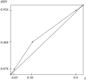
As an example, for the random prospect
d = [0,0.05 ; 0.5,0.25 ; 0.8,0.60 ; 1,0.10]
we obtain u = 0.705, P* = 0.3, and the following ki coefficients (cf formulae (2)
and (18)), given = 0.4:
k1 = 0.05(1 + 2×0.4×0.7) = 0.078
and analogously: k2 = 0.25×1.56 = 0.39, k3 = 0.6×0.76 = 0.456, k4 = 0.1×0.76 =
0.076 (note that k1 + ... + k4 = 1); hence q(p1) = 0.078, q(p1 + p2) = 0.468, q(p1 + p2 + p3) = 0.924, q(p1 + ... + p4) = 1. The concavity of the transformation function
is clearly appreciated from Figure 3. From both formulae (18) ug(d ) = 0.6358.
0.30 0.9 p 0.078 0.468 0.924 q(p) 0.05
7. EXPERIMENT
An experiment of the usual kind has been devised, asking twenty people (some colleagues and students of Economics) to answer ten questions of a question-naire, proposing games with only (limited) gains or nothing. The practical proce-dure was almost exactly borrowed from the one implemented by Tversky and Kahneman (1992, pp. 306-307).
The aim of the experiment (taking account of the small number of partici-pants) was not about revealing actual behaviour of people, but only about the op-erational control of model (5). The outcome of the experiment proved wholly successful. A detailed exposition of the experiment, together with its main results, is included in Section 10 of Frosini (2010).
Dipartimento di Scienze statistiche B.V. FROSINI
Università Cattolica del Sacro Cuore di Milano
REFERENCES
M. ALLAIS, (1953), Le Comportement de l’Homme Rationnel Devant le Risque: Critique des Postulats
et Axioms de l’Ecole Américaine, “Econometrica”, 21, pp. 503-546.
M. ALLAIS, (1988), The General Theory of Random Choices in Relation to the Invariant Cardinal
Util-ity Function and the Specific ProbabilUtil-ity Function. The (U,θ) Model. A General Overview, in:
Mu-nier B. (Ed.), Risk, Decision and Rationality,: Reidel, Dordrecht.
D. BERNOULLI, (1738/1954), Exposition of a New Theory on the Measurement of Risk (Translated
from Latin), “Econometrica” 22, pp. 23-36.
A. CHATEAUNEUF, M. COHEN AND I. MEILIJSON, (2005), More Pessimism than Greediness: A
Charac-terization of Monotone Risk Aversion in the Rank-Dependent Expected Utility Model,
“Eco-nomic Theory”, 25, pp. 649-667.
P.A. DIAMOND AND J.E. STIGLITZ, (1974), Increases in Risk and in Risk Aversion, “Journal of
Eco-nomic Theory”, 8, pp. 337-360.
J.S. DYER AND R.K. SARIN, (1982), Relative Risk Aversion, “Management Science”, 28, pp. 875-886. D. ELLSBERG (1961), Risk, Ambiguity, and the Savage Axioms, “Quarterly Journal of
Econom-ics”, 75, pp. 643-669.
I. FISHER, (1906), The Nature of Capital and Income. Macmillan: New York and London. B.V. FROSINI, (1984), Concentration, Dispersion and Spread: An Insight into Their Relationship,
“Sta-tistica”, 44, pp. 373-394.
B.V. FROSINI AND L. GIOSSI, (1994), La comparazione tra prospettive incerte: modelli teorici e
compor-tamento effettivo, Istituto di Statistica, Università Cattolica del Sacro Cuore, Serie E.P.
N.63.
B.V. FROSINI, (1997), The Evaluation of Risk Attitudes: A New Proposal, “Statistica Applicata”,
9, pp. 435-458.
B.V. FROSINI, (2010), Realistic Utility versus Game Utility: A Proposal for Dealing with the Spread of
Uncertain Prospects, Dipartimento di Scienze statistiche, Università Cattolica del Sacro
Cuore, Serie E.P. N. 140. http://dipartimenti.unicatt.it/scienze statistiche_statistiche_ 2183.html.
P. GÄRDENFORS AND N.E. SAHLIN, (1982), Unreliable Probabilities, Risk Taking, and Decision
B. HANSSON, (1988), Risk Aversion as a Problem of Conjoint Measurement, in: P. Gärdenfors,
N.E. Sahlin (Eds), Decision, Probability and Utility, Cambridge University Press, Cambri-dge, pp. 136-161.
D. KAHNEMAN AND A. TVERSKY, (1979), Prospect Theory: An Analysis of Decision under Risk,
“Econometrica”, 47, pp. 263-291.
J.M. KEYNES, (1921), A Treatise on Probability, Macmillan: London.
H.E. KYBURG, (1968), Bets and Beliefs, “American Philosophical Quarterly”, 5, (1968), pp.
63-78.
D.V. LINDLEY, (1985), Making Decisions (2nd edition), Wiley, London.
M. MACHINA, (1982), Expected Utility Analysis without the Independence Axiom, “Econometrica”,
50, pp. 277-323.
M. MACHINA, (1983), Generalized Expected Utility Analysis and the Nature of Observed Violations of
the Independence Axiom, in B. Stigum and F. Wenstǿp (Eds.), Foundations of Utility and Risk with Applications, Reidel, Dordrecht.
H. MARKOWITZ, (1952), The utility of wealth, “Journal of Political Economy”, 60, pp. 151-158. H. MARKOWITZ, (1959), Portfolio Selection, Wiley, New York.
J. MARSHAK, (1950), Rational Behavior, Uncertain Prospects and Measurable Utility,
“Economet-rica”, 18, pp. 111-141.
J. QUIGGIN, (1982), A Theory of Anticipated Utility, “Journal of. Economic Behavior and
Or-ganization”, 3, pp. 323-343.
J. QUIGGIN, (1985), Anticipated Utility, Subjectively Weighted Utility and the Allais Paradox,
“Or-ganisational Behavior and Human Performance”, 35, pp. 94-101.
J. QUIGGIN, (1991), Increasing Risk: Another Definition, in A. Chikan. (Ed.), Progress in Decision,
Utility and Risk Theory, Kluwer, Amsterdam.
J. QUIGGIN, (1993), Generalized Expected Utility Theory. The Rank-Dependent Model, Kluwer,
Boston.
J. QUIGGIN AND R.G. CHAMBERS, (1998), Risk Premiums and Benefit Measures for
Generalized-Expected-Utility Theories, “Journal of Risk and Uncertainty”, 17, pp.121-137.
J. QUIGGIN AND R.G. CHAMBERS, (2004), Invariant Risk Attitudes, “Journal of Economic
The-ory”, 117, pp. 96-118.
M. ROTHSCHILD AND J.E. STIGLITZ, (1970), Increasing Risk I: A Definition, “Journal of Economic
Theory”, 2, pp. 225-243.
L.J. SAVAGE, (1954), The Foundations of Statistics, Wiley, New York.
A. TVERSKY AND D. KAHNEMAN, (1992), Advances in Prospect Theory: Cumulative Representation of
Uncertainty, “Journal of Risk and Uncertainty”, 5, pp. 297-323.
J. VON NEUMANN AND O. MORGENSTERN, (1944/1953), Theory of Games and Economic Behavior
(3rd edition 1953), Princeton University Press, Princeton.
P. WAKKER, (1994), Separating Marginal Utility and Probabilistic Risk Aversion, “Theory and
De-cision”, 36, pp. 1-44.
M.E. YAARI, (1987), The Dual Theory of Choice Under Risk, “Econometrica”, 55, pp. 95-115. SUMMARY
Realistic utility versus game utility: a proposal for dealing with the spread of uncertain prospects
The author develops the properties and implications of a proposal, concerning a sum-mary statistic of the random prospect of utilities. Following a suggestion of Allais, such a statistic is increasing with expected utility, and decreasing – for most people, who are risk averse – with the mean absolute deviation of utilities; a parameter multiplying this
disper-sion measure allows for risk averse or risk prone behaviour, according to its sign, and also for more or less departure from a certain prospect. It is demonstrated that this statistic (a) satisfies the first stochastic dominance, (b) satisfies the independence condition, (c) satis-fies the so called “problem of probabilistic insurance”, (d) resolves the paradoxes of Al-lais, Ellsberg and Kahneman-Tversky (paradox of the substitution axiom), (e) is compati-ble with Quiggin’s approach of rank-dependent expected utility models, (f) the mean ab-solute deviation cannot be replaced by the standard deviation.