Università Politecnica delle Marche
Scuola di Dottorato di Ricerca in Scienze dell’Ingegneria Corso di Dottorato in Ingegneria Industriale
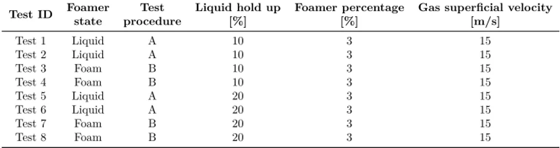
Flow Assurance Management: innovative
methodologies for Oil and Gas production
optimization
Ph.D. Dissertation of:
Davide Dall’Acqua
Advisor:
Prof. Giancarlo Giacchetta
Coadvisor:
Prof.ssa Barbara Marchetti
Curriculum Supervisor:
Università Politecnica delle Marche
Scuola di Dottorato di Ricerca in Scienze dell’Ingegneria Corso di Dottorato in Ingegneria Industriale
Flow Assurance Management: innovative
methodologies for Oil and Gas production
optimization
Ph.D. Dissertation of:
Davide Dall’Acqua
Advisor:
Prof. Giancarlo Giacchetta
Coadvisor:
Prof.ssa Barbara Marchetti
Curriculum Supervisor:
Ringraziamenti
Il dottorato mi ha dato l’opportunità di conoscere molte persone che hanno senza dubbio arricchito la mia vita sotto molteplici aspetti, per cui è doverso fare dei ringraziamenti.
Il primo grazie va a Mariella, per avermi aiutato con i suoi consigli nelle varie attività di ricerca, la quale ammiro sopratutto per il suo entusiasmo. Un debito grazie va a Barbara, Antonio e al prof. Giacchetta, per avermi introdotto ai moltemplici temi di ricerca e per avermi concesso di svolgere il dottorato in piena libertà. Un grazie lo devo a Valerio, per la sua disponibiltità nel dispensare consigli sulla termodinamica.
Sono ringraziati tutti i dottorati e dottorandi che ho avuto il piacere di conscere al DIISM e con i quali ho avuto modo di confrontarmi su temi di alta e bassa levatura. Un grazie in particolare è riservato ai miei compagni di ufficio. Maurizio, per il prezioso aiuto fornitomi nella fase sperimentale di laboratorio. Alex, per la sua disponibiltità e per la sua spiccata ironia che spesso mi ha rallegrato. Infine Laura, per la sua preziosa collaborazione nell’ultimo anno di dottorato.
Un grazie va a mia madre e mio fratello per supportarmi, oltre che sopportarmi. Infine, un grazie speciale lo riservo a mio padre, il cui ricordo è sempre stato fonte di forza per me durante questi anni, sperando che questo nuovo traguardo lo possa inorgogliere.
Ancona, November 2017
Abstract
Pipelines transport a variety of products, especially for energy purposes, such as natural gas, biofuels, and oil. The transportation of hydrocarbons through pipeline implies a wide number of problems. Engineers and operators have to carefully manage these problems in order to minimise the risk and ensure a safe and reliable transport. Although from the future energy outlooks the renewable sources are expected to grow with the highest rate, these will not be sufficient to cover the increasing energy demand and, new fossil sources will be required. The hydrocarbons coming from these sources will result more difficult to manage respect to the past, due to the end of the "easy-oil". With this perspective, the "Flow Assurance" holds an important role in the Oil&Gas industry of the future. This dissertation reports solutions obtained through three years of research activities for three important problems related to the hydrocarbons transportation through pipeline. These concern the investigation of a new method for the reduction of the liquid loading in pipeline transporting natural gas; the development of an algorithm for the calculation of the expansion wave curve in hydrocarbon and carbon dioxide gas mixtures; the evaluation of the reliability of wax deposition models implemented in commercial software for wax deposition prediction.
Contents
1 Introduction 1
1.1 Flow Assurance overview . . . 3
1.2 Flow Assurance analysis . . . 8
1.3 Analysed problems . . . 9
1.4 Outline . . . 11
2 Liquid loading issue 13 2.1 Literature review . . . 13
2.1.1 Natural gas . . . 14
2.1.2 Liquid loading in gas wells. . . 15
2.1.3 Liquid loading in pipelines. . . 22
2.1.4 Foamer injection in pipeline . . . 25
2.2 Surfactants and foam. . . 26
2.2.1 Foam structure . . . 27
2.2.2 Parameters influencing the deliquification through surfactant injection . . . 30
2.3 Experimental test bench description . . . 31
2.3.1 Test bench layout L1. . . 31
2.3.2 Test bench layout L2. . . 34
2.3.3 Test procedures . . . 37
2.4 Foam stability analysis . . . 40
2.4.1 Image processing code for foam decay analysis . . . 42
2.5 Experimental results . . . 50
2.5.1 Influence of the air superficial velocity . . . 50
2.5.2 Effects of the foam percentage on deliquification . . . 52
2.5.3 Deliquification capacity of preformed foam. . . 55
2.6 Stability analysis results . . . 58
2.6.1 Effects of different percentages of foamers . . . 58
2.6.2 Selection of the most suitable surfactant . . . 60
3 Calculation of the expansion wave velocity for natural gas mixtures 69
3.1 Literature review . . . 72
3.1.1 Codes calculating the expansion wave velocity. . . 76
3.1.2 Modelling CO2impure. . . 77
3.2 Thermodynamic . . . 78
3.3 Calculation model . . . 85
3.4 Expansion wave velocity for hydrocarbon gas mixtures . . . 93
3.4.1 Northern Alberta Burst Tests (NABT). . . 93
3.4.2 Tests performed at TransCanada PipeLines (TCPL) . . . 93
3.4.3 Tests HHVPG . . . 96
3.5 Expansion wave velocity for CO2-rich mixtures . . . 99
3.6 Conclusion . . . 108
4 Wax deposition in pipeline 109 4.1 Literature review . . . 110
4.1.1 Wax deposition overview . . . 110
4.1.2 Mechanisms involved in wax deposition . . . 113
4.1.3 Differences between single phase and multiphase flows . . . 116
4.1.4 Oil/Water Wax Deposition Studies . . . 121
4.1.5 Ageing of wax layer . . . 123
4.1.6 Effects of shear stress on deposit . . . 129
4.1.7 The importance of using a fully-compositional approach . . . . 132
4.1.8 Effect of deposit on pressure drop . . . 135
4.1.9 Wax layer porosity . . . 137
4.2 Wax deposition models. . . 137
4.2.1 RRR model . . . 139
4.2.2 Matazain model . . . 140
4.2.3 PVTSim wax module:DepoWax. . . 142
4.2.4 Infochem wax module: FloWax . . . 143
4.2.5 Michigan Wax Predictor (MWP) . . . 145
4.3 Analysed field data . . . 149
4.3.1 Petrobras data . . . 150
4.3.2 Statoil and TotalFinaElf data . . . 150
4.3.3 ConocoPhillips data . . . 162
4.4 Simulations results . . . 165
4.4.1 Results for Case1 . . . 166
4.4.2 Results for Case2 . . . 181
4.4.3 Results for Case3 . . . 187
4.4.4 Results for Case4 . . . 196
Contents
5 Appendix 207
5.1 Derivatives of the Peng-Robinson equation of state . . . 207
List of Figures
1.1 Total world energy consumption by energy source expressed in quadrillion
of Btu, 1990–2040 [2]. . . 2
1.2 Issues treated in Flow Assurance. . . 4
1.3 Parameters affecting the pipe flow. . . 5
1.4 Gas-liquid flow regimes in horizontal pipes. . . 6
1.5 Gas-liquid flow regimes in vertical pipes. . . 6
1.6 Scheme of the fluid route, from reservoir to separator, and various deposit zones. . . 7
1.7 Flow Assurance in the iterative process. . . 7
2.1 Gas well flowing in normal conditions. . . 16
2.2 Gas well affected by water coning. . . 16
2.3 Forces acting on a droplet as described by Turner’s model.. . . 19
2.4 Spherical drop and deformed drop in high velocity gas. . . 20
2.5 Severe slugging cycle in riser. (a) Blockage of the riser-base; (b) Liquid accumulation; (c) Sudden liquid surge; (d) Gas blowdown. . . 23
2.6 Pigging operation scheme. . . 24
2.7 Simple scheme of surfactant and surfactant disposition in solution. . . 27
2.8 Effect of the liquid volume fraction on a 2D foam. . . 28
2.9 Experimental and computer simulated dry foam (a,b); Experimental and computer simulated wet foam (c,d) . . . 28
2.10 Nanometric details of the plateau border visible in a picture obtained by a Cryo-Scanning Electron Microscope,(image credit N. Duerr-Auster, ETH, 2008). . . 29
2.11 3D representation of the modified MultiLab loop. . . 32
2.12 Test bench - Layout L1. . . 32
2.13 Representation of the variables used in Equation 2.16. . . 33
2.14 Test bench - Layout L2. . . 35
2.15 Preformed foam in the launching section. . . 35
2.16 Profile of the downward flexible pipe used in layout L2. . . 36
2.17 Radial fan and inverter used to generate the air flow. . . 36
2.18 Characteristic curve linking the inverter current frequency with the superficial air velocity measure through the pitot tube. . . 37
2.19 Foam into the pipe - Image taken by C8484-05C camera.. . . 41
2.20 Foam into the prototype case - Image taken by C8484-05C camera. . . 41
2.21 Scheme of the prism working principle. . . 43
2.22 Image of the built prototype beaker to analyse the foam decay. . . 43
2.23 Image of the foam seen through the prism.. . . 44
2.24 Scheme of the acquisition system.. . . 45
2.25 Foam domain identified by the code. . . 46
2.26 Liquid domain identified by the code. . . 46
2.27 Boundaries identification. . . 48
2.28 Identified boundaries and internal interpolation.. . . 48
2.29 Division of the foam domain in sub-domains for the correct selection of the conversion parameter.. . . 49
2.30 Minimum air superficial velocity request to have the local slug at the elbow without foamer. . . 51
2.31 Minimum air superficial velocity request to have the local slug at the elbow with foamer. . . 51
2.32 Effect of the foamer on the minimum air superficial velocities requested to have the local slug. . . 52
2.33 Percentages of liquid extracted from the system for different air flow velocities after a period of 120 s - 10% of liquid hold up (Layout L2). . 53
2.34 Percentages of liquid extracted from the system for different air flow velocities after a period of 120 s - 20% of liquid hold up (Layout L2). . 53
2.35 Percentages of liquid extracted from the system using different foamer percentages. Air velocity 15 m/s, observation time 120 s, liquid hold up 10%. . . 54
2.36 Percentages of liquid extracted from the system using different foamer percentages. Air velocity 15 m/s, observation time 120 s, liquid hold up 20%. . . 54
2.37 Percentage of liquid extracted from the system every 60 s using the foamer in the liquid state (A) and in preformed foam (B) - Liquid hold up 10%. . . 56
2.38 Total percentage of liquid extracted from the system using the foamer in the liquid state (A) and in preformed foam (B) - Liquid hold up 10%. 56 2.39 Percentage of liquid extracted from the system every 60 s using the foamer in the liquid state (A) and in preformed foam (B) - Liquid hold up 20%. . . 57
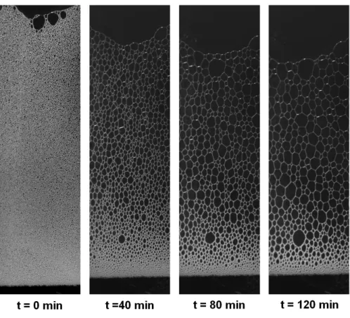
2.40 Total percentage of liquid extracted from the system using the foamer in the liquid state (A) and in preformed foam (B) - Liquid hold up 20%. 57 2.41 Four time frames showing the decay evolution of the foam.. . . 59
List of Figures
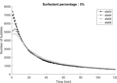
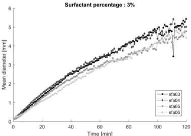
2.42 Surfactant sfa03 - Number of bubbles during the decay. . . 60
2.43 Surfactant sfa04 - Number of bubbles during the decay. . . 61
2.44 Surfactant sfa05 - Number of bubbles during the decay. . . 61
2.45 Surfactant sfa06 - Number of bubbles during the decay. . . 62
2.46 Surfactant sfa03 - Mean diameter during the decay.. . . 62
2.47 Surfactant sfa04 - Mean diameter during the decay.. . . 63
2.48 Surfactant sfa05 - Mean diameter during the decay.. . . 63
2.49 Surfactant sfa06 - Mean diameter during the decay.. . . 64
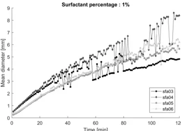
2.50 Surfactant percentage 1% - Comparison of the number of bubbles for the tested surfactants. . . 65
2.51 Surfactant percentage 3% - Comparison of the number of bubbles for the tested surfactants. . . 65
2.52 Surfactant percentage 6% - Comparison of the number of bubbles for the tested surfactants. . . 66
2.53 Surfactant percentage 1% - Comparison of the mean diameter for the tested surfactants. . . 66
2.54 Surfactant percentage 3% - Comparison of the mean diameter for the tested surfactants. . . 67
2.55 Surfactant percentage 6% - Comparison of the mean diameter for the tested surfactants. . . 67
3.1 Scheme of stresses acting on the pipe: axial stress σaand hoop stress σh. 70 3.2 Propagation of ductile fractures in pipeline [100]. . . 70
3.3 Example of two-curves model for the fracture arrest [38].. . . 74
3.4 Isentropic decompression prediction calculated by GASDECOM and phase envelope (BWRS EoS) for an hydrocarbon gas mixture [11]. . . 75
3.5 Expansion wave velocity calcualted by GASDECOM for an hydrocar-bon gas mixture [11]. . . 75
3.6 Multiple roots of a cubic equation of state . . . 79
3.7 Scheme of the calculation model. . . 86
3.8 Sound velocity versus void fraction in a two-phase homogeneous mix-ture [146]. . . 89
3.9 Effect of the sound velocity modelling on the expansion wave velocity for a light hydrocarbon gas mixture (MW = 19 g/mol). . . 91
3.10 Effect of the sound velocity modelling on the expansion wave velocity for a medium hydrocarbon gas mixture (MW = 20.3 g/mol). . . 92
3.11 Effect of the sound velocity modelling on the expansion wave velocity for a heavy hydrocarbon gas mixture (MW = 27.8 g/mol).. . . 92
3.12 Phase envelope (PE) and isentropic decompression (ID) path for each of the NABT gas mixtures. . . 94
3.13 Expansion wave velocity for the mixture NABT3. Comparison of PRDECOM and GASDECOM predictions against experimental data. 95
3.14 Expansion wave velocity for the mixture NABT5. Comparison of PRDECOM and GASDECOM predictions against experimental data. 95
3.15 Expansion wave velocity for the mixture NABT6. Comparison of PRDECOM and GASDECOM predictions against experimental data. 96
3.16 Phase envelope (PE) and isentropic decompression (ID) path for each of the TCPL gas mixtures. . . 97
3.17 Expansion wave velocity for the mixture Case4. Comparison of PRDE-COM and GASDEPRDE-COM predictions against experimental data. . . 98
3.18 Expansion wave velocity for the mixture Case6. Comparison of PRDE-COM and GASDEPRDE-COM predictions against experimental data. . . 98
3.19 Expansion wave velocity for the mixture Case8. Comparison of PRDE-COM and GASDEPRDE-COM predictions against experimental data. . . 99
3.20 Phase envelope (PE) and isentropic decompression (ID) path for each of the HHVPG gas mixtures. . . 100
3.21 Expansion wave velocity for the mixture HHVPG1. Comparison of PRDECOM and GASDECOM predictions against experimental data. 101
3.22 Expansion wave velocity for the mixture HHVPG2. Comparison of PRDECOM and GASDECOM predictions against experimental data. 101
3.23 Phase envelope (PE) and isentropic decompression (ID) for the mix-tures Test4, Test5 and Test6. . . 103
3.24 Phase envelope (PE) and isentropic decompression (ID) for the mix-tures Test7, Test8, Test9 and Test10. . . 104
3.25 Expansion wave velocity for the Test4. Comparison of PRDECOM and GERG2008 EoS predictions against experimental data. . . 104
3.26 Expansion wave velocity for the Test5. Comparison of PRDECOM and GERG2008 EoS predictions against experimental data.. . . 105
3.27 Expansion wave velocity for the Test6. Comparison of PRDECOM and GERG2008 EoS predictions against experimental data.. . . 105
3.28 Expansion wave velocity for the Test7. Comparison of PRDECOM and GERG2008 EoS predictions against experimental data.. . . 106
3.29 Expansion wave velocity for the Test8. Comparison of PRDECOM and GERG2008 EoS predictions against experimental data.. . . 106
3.30 Expansion wave velocity for the Test9. Comparison of PRDECOM and GERG2008 EoS predictions against experimental data.. . . 107
3.31 Expansion wave velocity for the Test10. Comparison of PRDECOM and GERG2008 EoS predictions against experimental data. . . 107
List of Figures
4.2 Wax deposition scheme. . . 112
4.3 Wax thickness distribution for various horizontal flow patterns [91].. . 117
4.4 Wax thickness distribution for various vertical flow patterns [91]. . . . 117
4.5 Thickness and hardness trends observed in horizontal flow tests [91]. . 118
4.6 Thickness and hardness trends observed in vertical flow tests [91].. . . 118
4.7 Average weight profile of deposits as a function of water cut [31]. . . . 122
4.8 Deposition rate versus water cut with methods A and B [153].. . . 123
4.9 Variation in the deposit mass at different water contents: effect of waxy mixture temperature (a), of coolant temperature (b) and of Reynolds number (c). . . 124
4.10 Deposition map for the two-phase oil/water system. . . 125
4.11 Internal pipe radius reduction due to deposit and wax content. . . 126
4.12 Enrichment of heavy waxy components during the course of wax depo-sition discovered by Singh et al. . . . 127
4.13 Comparison of wax deposit compositions as function of wall tempera-ture (Q = 21 m3/h). . . 127
4.14 Variation of wax yield stress with the applied shear stress. . . 131
4.15 The lumping effect on the wax precipitation curve using the Wilson wax model. . . 134
4.16 WPC using the Uniquac wax model with 15 n-paraffin pseudo-components.134 4.17 Lumping effect on deposition thickness profile. . . 135
4.18 Polarized light microscopy image of paraffin-oil gel. . . 138
4.19 Definition of wax content from gas chromatograph results. . . 138
4.20 Discretization of temperature profiles in the 1-D wax deposition models.145 4.21 2-D discretization of temperature profiles in the MWP.. . . 146
4.22 Flowline geometry Case1. . . 155
4.23 Case2 - Pipeline elevation profile. . . 156
4.24 Case3 - Pipeline elevation profile. . . 159
4.25 Case3 - Pressure drop and export rate. . . 161
4.26 Case4 - Weight percent distribution of n-alkanes and all hydrocarbons. 164 4.27 Case4 - Viscosity of the fluid. . . 164
4.28 Case4 - Samples of pipeline operation conditions. . . 165
4.29 Case1 - Comparison of the WPC generated by PVTsim Nova 3 and Multiflash 6.2. . . 167
4.30 Case1 - Pressure measurement at PDG. . . 168
4.31 Case1 - Wax deposition profile varying the diffusion coefficient multi-plier in OLGA. . . 170
4.32 Case1 - Pressure at PDG varying the diffusion coefficient multiplier in OLGA. . . 170
4.33 Case1 - Wax deposition profile varying the wax roughness in OLGA. . 171
4.34 Case1 - Pressure at PDG varying the wax roughness in OLGA. . . 171
4.35 Case1 - Wax deposition profile varying the deposition model in OLGA. 172
4.36 Case1 - Pressure at PDG varying the deposition model in OLGA.. . . 172
4.37 Case1 - Wax deposition profile varying the wax porosity in OLGA. . . 173
4.38 Case1 - Wax deposition profile varying the shear multipliers in OLGA. 173
4.39 Case1 - Pressure at PDG varying the shear multipliers in OLGA. . . . 174
4.40 Case1 - Pressure comparison between field data and OLGA simulation. 174
4.41 Case1 - Wax deposition profile over time in OLGA.. . . 175
4.42 Case1 - Wax deposition profile varying tfwall in LedaFlow. . . . 177
4.43 Case1 - Wax deposition profile varying tfwax in LedaFlow.. . . 177
4.44 Case1 - Wax deposition profile varying acwall in LedaFlow. . . . 178
4.45 Case1 - Wax deposition profile varying d23 in LedaFlow. . . . 178
4.46 Case1 - Comparison of wax deposition profiles of OLGA, LedaFlow and Depowax base cases. . . 180
4.47 Case2 - Fluid phase envelope using PVTsim 20. . . 182
4.48 Case2 - WPC reported from the paper.. . . 182
4.49 Case2 - WPCs comparison. . . 183
4.50 Case2 - Effect of the pressure on the WPC. Multiflash and PVTsim curve calculated at 120 bar. . . 184
4.51 Case2 - Fluid temperature profile predicted by OLGA. . . 185
4.52 Case2 - Pressure profile predicted by OLGA. . . 185
4.53 Case2 - Fluid temperature profile predicted by Deopowax. . . 186
4.54 Case2 - Pressure profile predicted by Depowax. . . 186
4.55 Case2 - Depowax wax deposition simulation after 168h. . . 187
4.56 Case2 - Wax deposition simulation predicted by Flowax after 168h. . . 188
4.57 Case2 - Comparison of wax deposition simulation. . . 188
4.58 Case3 - Fluid phase envelope using PVTsim 20. . . 189
4.59 Case3 - WPCs from the paper. . . 190
4.60 Case3 - WPCs comparison. . . 190
4.61 Case3 - OLGA wax deposition simulations. Wax table generated with PVTSim 20. Effect of shear removal option. . . 191
4.62 Case3 - OLGA wax deposition simulations. Wax table generated by Multiflash 6.1. Effect of shear removal option. . . 192
4.63 Case3 - LedaFlow wax deposition simulation. . . 192
4.64 Case3 - Depowax wax deposition simulation. . . 193
4.65 Case3 - Flowax wax deposition simulations. Effect of shear removal option. . . 194
List of Figures
4.67 Case3 - Wax deposit volumes collected after 11 days. . . 195
4.68 Case3 - Percentage deviations of the predicted wax deposit volume respect to the field data. . . 195
4.69 Case3 - Wax deposition profiles best fitting the measured wax volume. 196
4.70 Case4 - Extraction of the pressure trend after each pigging operation. 197
4.71 Case4 - WPC calculated with different software. . . 197
4.72 Case4 - OLGA wax deposits comparison. . . 199
4.73 Case4 - Pressure drop predicted by OLGA. . . 199
4.74 Case4 - Pressure drop predicted by OLGA tuning wax deposition pa-rameters. . . 200
4.75 Case4 - Wax deposit predicted by LedaFlow. . . 200
4.76 Case4 - Wax deposit predicted by Depowax. . . 201
4.77 Case4 - Wax deposit predictions calculated by Flowax. . . 202
4.78 Case4 - Pressure drop predicted by Flowax. . . 202
4.79 Case4 - Pressure drop prediction by Flowax tuning the mass transfer coefficient. . . 203
List of Tables
1.1 Energy required for different transportation types. . . 3
2.1 Typical compositions of dry and wet gases [mol%] [86]. . . 15
2.2 Comparison between pigging and foaming. . . 26
2.3 Characteristics of loop layout L1 . . . 32
2.4 Summary of the performed test to investigate the effect of foamer per-centage on deliquification . . . 53
2.5 Summary of performed test to evaluate the influence of the foamer state on the deliquification. . . 55
2.6 Physical properties of the tested surfactants. . . 58
3.1 Values of the binary interaction parameters used in Van der Waals mixing rule. . . 81
3.2 Peneolux correction factors. . . 82
3.3 Coefficients for the calculation of the ideal isobaric heat capacity CP,i0 . 83
3.4 NABT - Fluids molar compositions. . . 94
3.5 NABT - Fluids initial conditions. . . 94
3.6 TCPL - Fluids molar compositions.. . . 97
3.7 TCPL - Fluids initial conditions. . . 97
3.8 HHVPG - Fluids molar compositions. . . 100
3.9 HHVPG - Fluids initial conditions. . . 100
3.10 Carbon dioxide rich mixtures - Molar compositions. . . 102
3.11 Carbon dioxide mixtures - Initial conditions. . . 103
4.1 Case1 - Materials properties. . . 150
4.2 Case1 - Walls definition. . . 151
4.3 Case1 - Composition of the liquid phase. . . 152
4.4 Case1 - Composition of the vapour phase. . . 153
4.5 Case1 - Composition of the mix. . . 154
4.6 Case1 - Molar composition of wax fractions. . . 154
4.7 Case1 - Main characteristics. . . 155
4.8 Case2 - Pipeline materials.. . . 156
4.10 Case2 - Operational data. . . 157
4.11 Case2 - Main characteristics. . . 158
4.12 Case3 - Pipeline materials.. . . 159
4.13 Case3 - Composition of the fluid. . . 160
4.14 Case3 - Physical properties of the oil. . . 161
4.15 Case3 - Main characteristics. . . 162
4.16 Case4 - Summary of pipeline design parameters. . . 163
4.17 Case4 - Composition of the fluid. . . 163
4.18 Case1 - Values of wax deposition parameters used in OLGA. . . 168
4.19 Case1 - Values of wax deposition parameters used in LedaFlow. . . 176
4.20 Case1 - OLGA default value for wax deposition. . . 179
4.21 Case1 - LedaFlow default value for wax deposition. . . 180
4.22 Case1 - Depowax default value for wax deposition. . . 180
Chapter 1
Introduction
Humankind, since the dawn of time, has been able to master different forms of energy and transform them to improve the quality of life. Today, the energy mix is a trade-off between multiple sources, as we are able to convert them in many ways in order to power high-consuming societies. The outlook for energy use worldwide presented in different studies report a rising levels of demand over the next three decades, led by strong increases in countries such as Asia, China and India [2, 15]. The increment of energy consumption is strictly related to population and economic wealth growth. By 2035, the world’s population is projected to reach 8.7 billion, which means an additional 1.6 billion people will need energy [15].
As shown in Figure 1.1, renewables have been predicted as the world’s fastest growing energy source for a projection extended up to 2040, with an average increase by 2.6% per year between 2012 and 2040. Even though consumption of non-fossil fuels is expected to grow faster than consumption of fossil fuels, a projection of fossil fuels still account for 78% of energy use in 2040. Liquid fuels, mostly petroleum-based, are expected to remain the largest source of energy consumption, even if a reduction of liquid fuels consumption from 33% to 30% is predicted. On the other side, an increment of natural gas consumption, due to abundant natural gas resources, such as shale gas, tight gas and coalbed methane, contribute to a strong competitive position in the energy market. While coal is expected to be the slowest growing fuel, as environmental policies around the globe tighten.
In the past, the world has been accustomed to cheap fossil fuel, the so called "easy oil", intending reserves easy to find, easy to extract from the ground and easy to transform into ready-to-consume products. The easily recoverable oil is either gone or continues to be depleted. Since the mid-20th century, the most important oil and natural gas reserves have been discovered in the Middle East. This region, led by Saudi Arabia, Iran, Iraq, Kuwait and the UAE represents almost half of the world’s proven oil reserves. For natural gas, notably thanks to Iran and Qatar, the Middle East holds 43% of the global reserves. Lately Venezuela and Canada reserves have been recently reassessed and have increased dramatically, now ranking first and third
Figure 1.1: Total world energy consumption by energy source expressed in quadrillion of Btu, 1990–2040 [2].
for proven oil reserves. Nevertheless, the most recent oil discoveries have been made in unfamiliar locations, such as deep water and ultra-deep water. The offshore field exploitation has changed dramatically from the 1950s, where hydrocarbon production at an industrial level commenced at water depths of tens of meters in the Gulf of Mexico. The interest in offshore hydrocarbon production was greatly boosted by the oil crisis of 1973, and European countries, such as the United Kingdom and Norway, began to exploit hydrocarbons at water depths between 100 m and 150 m. Offshore technology has progressively improved, and it is now possible to extract oil or gas at water depths exceeding 3000 m [103].
Nowadays the hydrocarbon sources can be divided in two categories: conventional and unconventional. Conventional is referred to general hydrocarbons that can be produced from sources with little or no effort. To be identified as conventional, the source needs the 40% or more of the fluids it contains should be hydrocarbons; the underground pressure and temperature should be high enough for the hydrocarbons to reach the surface on their own [110].
The energy market to face the growing request of energy it has been taken in con-sideration also unconventional hydrocarbons, such as heavy, extra-heavy oils, tight oils, and tar sands. These heavy oils and extra-heavy oils have a high density and a very high viscosity, therefore they cannot be extracted using conventional methods, but they require more sophisticated techniques for their exploitation. These new
chal-1.1 Flow Assurance overview
Mode of Transportation Energy Consumption [BTU/Ton-mile] Airplane 37,000 Truck 2,300 Railroad 680 Waterway 540 Oil pipeline 450
Table 1.1: Energy required for different transportation types.
lenging sources of hydrocarbon request new technologies and a more detailed study, to prevent losses, mitigate risk and guarantee a safety and continuous production.
The term Flow Assurance was first coined by PETROBRAS in the mid 80’s [22] in Portuguese as Garantia do Escoamento, meaning literally "Guarantee of Flow". It entails design tools, methods, equipment, knowledge and professional skills needed to ensure the safe, uninterrupted transport of reservoir fluids from the reservoir to pro-cessing facilities. Problems arising in the transportation of hydrocarbons by pipelines from reservoir to downstream facilities can be manifold and of various nature con-sidering the whole life of the filed. In addition, the dependability of the problems [35], i.e. possible interactions among phenomena, can give rise to more risky scenario, both for the environment and the human life. Within this prospective it is clear the importance of the Flow Assurance for future petroleum production characterized by many uncertainties.
1.1 Flow Assurance overview
Transmission pipelines are the arteries of oil and gas industry, transporting the hy-drocarbons from the wells to locations where they are used as fuels or where they are refined into useful products. Pipelines are the most convenient method for trans-porting large quantities of crude oil and gas, having the following advantages: the transportation cost is lower than other modes of transportation; the energy required to operate the pipelines is lower than that required to operate other modes of trans-portation, seeTable 1.1[110].
Understand how the flow behaves is essential in the petroleum industry, so it is fundamental evaluate the all the variables that could affect the fluid flow from inlet to outlet. Figure 1.2reports a scheme summarizing some of these problems typical of the hydrocarbon production.
The Flow Assurance team’s analysis dictates the operating philosophy and oper-ating strategies for managing these problems. These phenomena can affect the sys-tem operability for all production modes, including start-up, normal operation, rate
Figure 1.2: Issues treated in Flow Assurance.
change and shut-down throughout the system life cycle. Engineers can rely on several software, which have been developed to simulate and analyse complex scenario. Such complexity depends on what the pipe transports and what sort of phenomena we want to investigate.
A pipeline transport system can be identified according to the following classifica-tion:
• Export pipelines: single-phase flow oil, gas, water
• Flowlines: multi-phase fluids (oil, gas, water) for gathering and injection system • Trunk lines: multi-phase fluids (oil, gas, water) for gathering and injection
system
• Special transport pipelines: solid/liquid slurries, waxy crude oil, multi-products. In Figure 1.3 is reported a scheme with most of the variables that user has to consider for a correct simulation of the flow in pipeline transporting hydrocarbons. To define a flow simulation, the type of flow model has to be defined first: single-phase (oil, gas, water) or multi-phase (oil-gas, oil-water, oil-gas-water).
Multi-phase flow has been first studied in nuclear plants, nevertheless also the hydrocarbon production more and more often exploits this type of flow. For example, using multi-phase flow to send produced gas, oil and water to shore directly can be much cheaper than offshore separation [14]. One of the most challenging aspects
1.1 Flow Assurance overview
Figure 1.3: Parameters affecting the pipe flow.
of dealing with multi-phase flow is the fact that it can take many different forms.
Figure 1.4illustrates the flow regimes encountered in horizontal two-phase gas-liquid flow. Stratified flow has the strongest tendency to occur in downhill or horizontal flow with relatively small gas and liquid flow rates. Increasing the gas velocity, waves start to form, and these waves can get high enough to reach the top of the pipe. When that happens, the gas is throttled or even blocked for a moment so that the flow becomes discontinuous, thus leading to the formation of slugs or elongated bubbles.
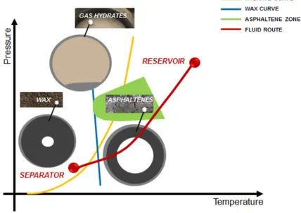
Figure 1.5 illustrates gas-liquid flows in vertical pipe, which are similar to those in horizontal pipes, but with the difference that stratified flow is not possible in vertical pipes. The slug flow is a typical fluid dynamic problem in Flow Assurance. Due to the periodic accumulation of liquid it changes from time to time, resulting detrimental for production because of the high variations of pressure it generates. Moreover, it can also lead to gas and liquid arriving at the processing facilities unevenly, causing tanks to flood. Solid deposition represents one of the main risk of petroleum production. It can generate plugs in the pipe or deposits along the walls of the well. It includes hydrates, wax, asphaltene, or emulsions. A direct consequence of the deposit is a reduction of the surface available for the fluid to flow, which in some extreme cases can lead to the flow interruption. In Figure 1.6 is illustrated a typical route of a fluid, from the reservoir to the separator. At the reservoir conditions the fluid is at high pressure and temperature, but when it starts to flow along the pipeline this is subjected to a cool down, due to lower temperature of the environment with respect to the fluid one. The reduction of temperature of the fluid can lead to the formation of new phases, such as waxes or hydrates. Such deposits are mainly governed by low temperatures, but it depend also on the fluid compositions and other conditions. For example, the hydrates formation begins when natural gas at high pressure and low temperature comes in contact with liquid water, where typical conditions are 20◦C and 100 bara.
To reduce the risk in hydrocarbons production, the Flow Assurance assessment should be thought as an iterative process [47], see Figure 1.7, starting from the Ex-ploratory phase, where no fluid sample is available and a first assessment has to be
Figure 1.4: Gas-liquid flow regimes in horizontal pipes.
1.1 Flow Assurance overview
Figure 1.6: Scheme of the fluid route, from reservoir to separator, and various deposit zones.
performed based on hypothesis. Once the fluid composition has been estimated and the production system has been sketched, a basic scenario can be defined. At this stage the main risks involved in the system can be defined. Passing to the Develop-ment phase of the system new information are available, and the basic scenario can be corrected and further detailed. Once the system starts to produce, Operation phase, the Flow Assurance assessment can be improved to understand where the system does not work as conceptualised.
1.2 Flow Assurance analysis
The aforementioned problems could be avoided with an accurate analysis of the sys-tem. The Flow Assurance analysis of a pipeline could be divided in two main stages [139]:
• Steady-state flow conditions: within this analysis the size and thickness of the pipelines is defined in order to minimize the pressure losses and optimize the performances of the system at the pipeline inlets (delivery pumps, compressors). During this phase are also defined the inlet and outlet pressures and temperature of the pipelines.
• Transient-flow conditions: in this stage is evaluated the dynamic behaviour of the system during flow variations, conditions met in start-up, shut-down, production rate change and pigging operations. The blowdown operation has to be analysed to evaluate the discharge rates, duration, pipeline internal pressure, temperature and inventory evolutions.
The steady-state analysis and the transient analysis are characterised by the fol-lowing sequence of tasks:
1. Thermodynamic characterization of the fluid: in this task the thermodynamic properties of the fluid request in the transport analysis are characterised. 2. Definition of pressure constraints: the maximum operation pressure (MOP)
at the system inlet is defined on the basis of design pressure; estimation of concentrated pressure drop along the transport system; specification of delivery pressure.
3. Steady-state flow simulations at maximum flow: these are performed to define the pipeline size according to:
• Pipeline inlet pressure: the maximum required inlet pressure for a pipeline must not exceed the MOP
• Fluid velocity: the liquid velocity in pipeline must not exceed 4 m/s, with an optimal operating rage of 1-2 m/s. The gas velocity must not exceed 20 m/s, with an optimal operating range of 5-10 m/s.
• Erosion velocity: the erosion velocity must not exceed the unity.
Multi-phase pipeline can require also steady-state simulation to identify possible flow instabilities as the aforementioned slugging. Also turn-down conditions are inves-tigated (30% of design flow) to evaluate possible flow instabilities. With multi-phase flows the maximum pressure drop is not necessarily at maximum total flow condition,
1.3 Analysed problems
therefore a number of production reference years are identified for the analysis, such as: maximum gas flow, maximum gas/oil ratio (GOR), maximum total liquid flow, maximum oil flow, maximum water flow.
1.3 Analysed problems
Several problems concerning the petroleum production are still unsolved or partially understood. In this dissertation three different problems affecting the hydrocarbon transportation in pipeline have been studied:
• Liquid loading in pipeline transporting natural gas,
• Modelling of the expansion wave curve in high pressurised pipeline transporting natural gas,
• Wax deposition in pipeline.
These issues have been chosen in collaboration with ENI and SAIPEM, respectively the major Italian oil company and one of the most important Italian Oil&Gas engi-neering contractor. Hereinafter is given a general description of these topics with the research objective.
Liquid loading in pipeline transporting natural gas
Experimental campaigns at the laboratory of the Università Politecnica delle Marche have been carried out to investigate a new liquid removal technique for pipeline trans-porting natural gas. Such technique uses chemicals, more precisely surfactants, which taking advantage of the foam characteristics should be able to deliquify the system. The resulting flow is composed by three phases (water, gas, foam), due the flow complexity and the numerous variables that could affect the result, an experimental campaign on a test loop developed for multi-phase flow research was requested. Sev-eral tests have been conducted imposing different geometries, operational conditions and surfactant types. Common soap and products developed for application in field have been tested in laboratory. The obtained results showed that the application of this technique has the potentiality to solve the liquid loading issue, or at least to lessen it, if some conditions are met. This technique cannot be substitute for the normal pigging operations, since this is not able to remove solid deposits, but it should be used in synergy with the latter to maximise the production.
Objectives: Evaluate the variables affecting the deliquification and their impact on the deliquification rate, in order to maximise the deliquification through surfactants.
Calculation of the expansion wave curve for ductile fracture control in pipeline
The calculation of the expansion wave curve is a problem linked to the ductile fracture propagation in pipeline transporting high pressurised natural gas. A ductile fracture cannot be prevented in any case, and in the unfortunate case of pipeline failure, the pipeline decompression study could be useful to evaluate if the fracture remains con-fined or if it starts to propagate indefinitely. This problem was first solved at the Battelle Memorial Institute developing the so called "two-curves model" [38]. This is a multi-physics method, since it combines the model of the velocity propagation of a ductile fracture and the model of the velocity of the expansion wave in the pipe, both functions of internal pipe pressure. The expansion wave curve highly depends on the fluid composition and operational conditions. In the following study a Matlab code has been developed to predicted the expansion wave velocity of natural gas mixtures. The thermodynamic properties of the code have been calculated using the Peng-Robinson equation of state. The code have been validated against curves predicted with other equations of state and with experimental data available in literature. In particular, it has been demonstrated that the Peng-Robinson is able to provide good results in term of expansion wave velocity, especially for CO2-rich mixtures, where
nowadays there is not yet a reference equation of state for such compositions.
Objectives: Assess the capability of the PR EoS to predict the expansion wave curves for hydrocarbon gas mixtures and CO2-rich mixtures.
Wax deposition in pipeline
Wax deposition has become one of the most common Flow Assurance problems in the petroleum industry, as reservoirs shift from onshore toward offshore subsea pro-duction. The industry is currently facing unprecedented challenges to maintain Flow Assurance for petroleum production, in which the strategy to prevent or mitigate wax deposition has become increasingly costly and complicated [61], making it a billion dollars problem. Until today oil companies have invested a lot of resources to un-derstand the phenomena governing wax deposition, but although several steps have been done, several aspects remain unsolved or not fully understood. Within this con-text a deep evaluation of the capabilities of commercial thermodynamic software and thermo-hydraulic software modelling the wax deposition has been carried out. The results of the simulations performed with the software have been compared with real field data available in literature.
Objectives: Analysis of the different models developed for wax deposition prediction and evaluation of their performances against field data.
1.4 Outline
1.4 Outline
The thesis has been divided in accord with the three main topics studied along the three years. The second chapter introduces the problem of liquid loading in pipeline transporting natural gas. A solution to this problem, based on surfactant injection, is presented. The chapter reports the descriptions and the results of two experimen-tal campaigns performed on a laboratory test bench, and the results of foam decay obtained through a code based on image processing.
The third chapter deals with the calculation of the expansion wave velocity in pipeline transporting natural gas mixtures. This topic is related to the ductile fracture control in pipeline. An algorithm developed for the calculation of the expansion wave curve is presented, in addition to comparisons of the obtained results against experimental data and literature data. The code has been tested for hydrocarbon gas mixtures and carbon dioxide mixtures.
In the fourth chapter the wax deposition issue in pipeline transporting waxy crude oil is analysed. A review of wax deposition models and the influence of some important parameters on wax deposition is presented. Four real cases, available in literature, have been selected to evaluate the capabilities of wax deposition models implemented in commercial software to predict wax deposit. The chapter reports some of the performed analysis for the cited cases.
Chapter 2
Liquid loading issue
The liquid loading could be described as the inability of the system to bring liquid out of the system. This is a typical problem affecting gas wells, especially old gas well, in which the gas production is low due to the reservoir depletion. In such systems the bottom-well starts to accumulate liquid, giving rise to an hydrostatic head acting on the reservoir and consequently reducing the production flow rate. Several techniques have been developed to solve or reduce the liquid loading problem in well. Although in literature most of the attention has been placed on wells, also pipelines transporting natural can be affected by liquid loading, especially if these lie on hilly terrains. A direct consequence of the accumulation of liquid is a higher pressure drop generated by a reduction of the gas flowing area. Nevertheless, this is not just a problem concerning the production, since accumulated liquid trapped for long time in the pipeline can originate rust, weakening dangerously the pipe walls.
2.1 Literature review
The liquid loading is a typical issue for old gas well. The accumulated liquid on the bottom of the well creates an hydrostatic head on the reservoir, resulting detrimental for the production and shorting the life of the well. If the liquid is not removed from the bottom well, the accumulated liquid can lead to a premature death of the well. To prevent such problem is fundamental to recognise when the well will undergo this phenomenon and act in order to prevent erratic production. When the gas flow rate is high, the liquid coming out from the well bore is transported in the gas stream up to the well head. The reservoir pressure decrease with the life of the well, leading to low flow rate, where the low gas velocity is not be able to transport the liquid up to the well head. Turner [142] calculated the minimal gas flow rate requested to maintain a liquid droplet suspended in a gas stream. Subsequently Nossier [106] and Li [79] improved the model of Turner considering the influence of other parameters, such as the flow regime and shape assumed by a droplet in a gas stream.
reduce the accumulated liquid in the well, such as plunger, velocity string, gas lift, etc. Among these, the application of surfactant in the bottom well represents one of the most economic technique. Nevertheless, a careful analysis has to be carried out in order to identify a good compromise between the costs and benefits [75].
The liquid loading is an issue influencing also the transport of hydrocarbons in pipeline. Usually the liquid and solid deposits are removed through the pigging oper-ation, which can be considered a consolidated technique. The pig is a capsule shape device, which acts like a piston pushing the accumulated deposit out of the pipeline. This maintenance operation is considered risky, due to the possibility to have a stuck pig, and not always applicable, due to the presence of butterfly valves, ball valves, etc. The use of surfactants injection has recently applied also in pipeline to remove liquid deposit [111]. In literature there are very few papers reporting application of such technique in pipeline, and none describing when or how to apply it to maximise the deliquification success rate. The surfactants should be used in synergy with the pigging operation, since it can remove solid deposit.
2.1.1 Natural gas
There is no one composition or mixture that can be referred to as natural gas, since each gas stream has its own composition. Two wells from the same reservoir can have two different compositions, moreover such compositions can change with the reservoir depletion, so the composition has to be analysed several times during the life of the well.
The natural gas can be divided in two main categories: • associated gas: gas produced in association with crude oil; • non-associated gas: gas is produced without oil .
The non-associated gas is produced only if it is possible to sell this latter on the market. Originally the associated gas was considered a waste product coming from the oil production, for such reason it was flared. Today, for the environmental policies and energetic concerns, it is no more allowed and it is considered a feedstock. A natural gas can be defined either sour or sweet, depending on the amount of carbon dioxide and hydrogen sulphide present in the gas. When the gas has an high amounts of sulphur compounds, especially H2S, it is called sour. A sour gas implies corrosion
issues, so it requests more expensive materials to be transported. While the CO2and
N2 reduce the quality of the gas, affecting the its selling price.
The natural gas mixture can be also defined wet or dry, depending on its composi-tion. Such distinction it is made on the amount of higher hydrocarbons present in the gas. A low amount of higher hydrocarbons makes the gas free of condensate, so it is
2.1 Literature review
Component Dry gas Wet gas
Hydrocarbons C1 70–98 45–92 C2 1–10 4–21 C3 Trace–5 1–15 C4 Trace–2 0.5–7 C5 Trace–1 Trace–3 C6 Trace–0.5 Trace–2 C7+ Trace–0.5 Trace–1.5 Non-Hydrocarbons N2 Trace–15 Trace–10 CO2 Trace–5 Trace–4 H2S Trace–3 0–6 He Trace–5 0
Table 2.1: Typical compositions of dry and wet gases [mol%] [86].
defined dry. On the other hand, when the condensation of higher hydrocarbons occurs at ambient temperature, the natural gas is defined wet. The typical composition of dry and wet gases are given inTable 2.1.
2.1.2 Liquid loading in gas wells
The liquid loading problem has been first experienced in old gas well, where the deple-tion of the reservoir, with a consequent pressure reducdeple-tion, gave rise to accumuladeple-tion of liquids at wellbore. The liquid loading of a gas wells could be described as the inability of the produced gas to remove the produced liquids from the wellbore [75]. Liquids can come from condensation of gas hydrocarbon (condensate) or from water in the reservoir matrix. As the velocity of the gas in the well drops with time, the velocity of the liquids carried by the gas decreases even faster. As a result, liquids begin to collect on the walls of the conduit, liquid slugs begin to form, and eventually liquids accumulate in the bottom of the well. The presence of liquids at the wellbore adds a back pressure on the reservoir, affecting the production of the well. In high pressure gas well the regime flow can turn in a slugging or churning flow, slowing down the production, while in low pressure wells it can even kill the well. The reduction of production can be evaluated through the flowing tubing pressure (FTP), which can be calculated as follow
F T P =Pres−∆PW −∆Ph−∆Pf ric (2.1) where:
Figure 2.1: Gas well flowing in normal conditions.
Figure 2.2: Gas well affected by water coning.
Pres =reservoir pressure
∆PW =pressure losses near-wellbore ∆Ph =hydrostatic pressure
∆Pf ric=pressure losses due tubing friction
While the hydrostatic pressure increases with the liquid accumulation, the pressure losses due to the tubing friction decreases due to reduced flow. When the hydrostatic pressure increases more than the decrement of pressure due to friction, then the F T P starts to reduce and the well slows down its production.
The liquid loading is a problem that each gas well will experience during the whole production life, the only exception can be made for completely dry gas wells, but these are very few. Therefore, the liquid loading has to be taken into account during the design phase of the well, and it becomes essential to have tools to predict the phenomenon.
Sources of liquid in well
Many wells produce not only hydrocarbons but also produced water. Produced water is water trapped in underground formations that is brought to the surface during oil and gas exploration and production. Produced water is by far the largest volume byproduct stream associated with oil and gas production. In traditional oil and gas wells, produced water is brought to the surface along with oil or gas. Another liquid source in well are hydrocarbon condensates, i.e. hydrocarbons entering the well in the vapour phase, that turn out in liquid phase due to change of pressure and temperature along the tubing.
The liquid sources affecting production in gas wells may be different: • Water coning
Water may be coned in from an aqueous zone above or below the producing zone. If the gas rate of a well is high enough, the gas may pull water production
2.1 Literature review
from an underlying zone, even if the well is not perforated in the water zone. This phenomenon affects largely also oil wells. Under ideal conditions in which no coning exists, flow is principally horizontal and mainly gas is produced.
Figure 2.1illustrates a producing well with no coning. When coning exists, the bottom-water is drawn upward in the producing zone. Figure 2.2illustrates a well subjected to coning.
• Aquifer water
If the reservoir has aquifer support, the encroaching water will eventually reach the wellbore.
• Water produced from other zone
Water may enter the wellbore from another producing zone, which could be separated some distance from the gas zone.
• Free formation water
It is possible for water to enter the well through the perforations with the gas. • Water and hydrocarbons condensation
Considering a gas well producing wet gas, if the reservoir pressure has decreased below the dew point, condensate is produced with the gas as a liquid; if the reservoir pressure is above dew point, the condensate enters the wellbore in the vapour phase with the gas and drops out as a liquid in the tubing or separator when the pressure drops. Like for condensates, also water exhibits the same behaviour.
Critical velocity
The liquid loading phenomenon was investigated first by Turner [142], who proposed two physical models to describe the liquid loading in gas well:
• Liquid film model: it considers a liquid film moving along the pipe wall • Drop reversal model: it considers liquid droplets entrained in high velocity gas
stream
Turner proved that the drop reversal model was more adequate for explaining load-up of gas wells. The key parameter of the droplet reversal model is the critical velocity. When the gas velocity is above the critical velocity, the droplets move upward the well; unlikely when the gas velocity is below the critical velocity the droplets fall back in the well, giving rise to the liquid accumulation. This model can be applied to vertical and near vertical conduit. The model is based on the balance of two forces acting on the liquid droplet: the weight force and the drag force due to the gas flow.
InFigure 2.3is reported a sketch of the two forces acting on a droplet in a vertical conduit. The weight acts downward, the drag force acts upward. When the drag force balances the weight force, the velocity of the gas stream is critical. Theoretically, at critical velocity the droplet would be suspended in the gas stream, moving neither upward nor downward. Turner calculated the drag force FDand the gravity force FG as follow FG =g(ρl− ρg) πd3 6 (2.2) FD = 1 2ρgCDAd(vg− vd) 2 (2.3) where : g =gravity acceleration ρl =liquid density ρg =gas density d =droplet diameter CD=drag coefficient
Ad =droplet projected cross-sectional area
vg =gas velocity
vd =droplet velocity
The critical velocity is obtained when the droplet velocity is null vd = 0. The assumed droplet is simplified to a sphere shape, so the cross-sectional area is calculated as Ad =πd2/4. Making equal FG and FD is possible to express the critical velocity
vc as vc= √ 4g(ρl− ρg)d 3ρgCD (2.4)
Equation 2.4 requires a known droplet diameter. Looking to the equation, the larger the drop, the higher the gas velocity necessary to hold it suspended is. So, the problem is to define the diameter of the largest drop that can exist in a given flow filed. Hinze [55] demonstrated that liquid drops moving relative to a gas are subjected to forces that try to shatter the drops, while the surface tension of the liquid acts to hold the drop together. He determined that it was the antagonism of two pressure, the velocity pressure, v2ρg, and the surface tension pressure, σ/d. The ratio of these two pressures is the dimensionless Weber number NW E.
For free falling drop the critical number was found to be between 20 and 30. If this critical value is exceeded a liquid drop should shatter [55]. The largest drop diameter
2.1 Literature review
Figure 2.3: Forces acting on a droplet as described by Turner’s model.
was obtained using the highest value, as follow
NW E=
v2cρgd
σgc
=30 (2.5)
In theEquation 2.5the variables are expressed using the English Engineering System of Units (English units), where gc represents the gravitational constant.
Expressing the droplet diameter in terms of NW E it is possible to write the critical velocity as vc= ( 40gcg CD )1/4( ρ l− ρg ρ2 g σ )1/4 (2.6) Turner assumed a drag coefficient CD=0.44, such value is valid for fully turbulent conditions. Expressing the surface tension σ in dyne/cm the equation can be written as showed inEquation 2.7 vc =1.593 ( ρl− ρg ρ2 g σ )1/4 (2.7)
Turner’s correlation was tested against a large number of real well data having surface flowing pressures mostly higher than 1000 psi (≈ 69 bar) and he found that the best fit respect to experimental data was obtained adjusting the critical velocity value 20% upward. vc=1.2 · 1.593 ( ρl− ρg ρ2 g σ )1/4 (2.8) Later on, Coleman [23] developed a relationships for the minimum critical flow rate similar to the model of Turner. Coleman tested his formula against gas wells having a pressure lower than 1000 psi and he found the best fit for experimental data removing
Figure 2.4: Spherical drop and deformed drop in high velocity gas.
adjustment factor of 20%.
Nosseir et al. [106] adopted the Turner’s basic concepts, but they focused on the impact of flow regimes in gas well. Turner assumed a single drag coefficient CD=0.44, while Nosseir assumed drag coefficients based on Reynolds number (NRe). In low pressure and flow rate well, with a NRebetween 2 · 105to 106, a transition flow might occur. In such case a drag coefficient of 0.44 is used, leading to the critical velocity reported inEquation 2.9, where µG represents the gas viscosity. In highly turbulent flow regime, NRe greater than 106, the drag coefficient value is set to 0.2 leading to
Equation 2.10. In bothEquation 2.9andEquation 2.10the parameters are expressed using the English units.
vc=14.6 σ0.35(ρl− ρg)0.21 ρ0.426 g µ0.134G (2.9) vc=21.3 σ0.25(ρl− ρg)0.25 ρ0.5 g (2.10) It was found that there are many gas wells producing rate much below the minimum flow rate calculated from Turner’s critical velocity and these wells still keep in good production state in China. Li et al. [79] state that the critical velocity proposed by Turner was not considering the deformation of liquid droplets in high velocity gas stream, due to a pressure difference between the fore and aft portions of the drop. Such pressure difference deforms the drop shape, changing from spherical to the shape of a convex bean, as showed in Figure 2.4. A drop having a convex bean shape is easier to lift respect to a spherical shape, thanks to a larger portion of area offered to the gas stream, therefore the calculated critical velocity to maintain suspended the droplet results minor than Turner one. The model developed by Li calculates the critical velocity as showed inEquation 2.11, expressing the parameters through the SI units.
vc=2.5
σ1/4(ρl− ρg)1/4
ρ1/2g
2.1 Literature review
Techniques for liquid removal in well
A typical gas well continues to produce for a period of 15-20 years. Along the life most of the wells will experience a liquid loading issue, even if the tubing size have been selected correctly. Liquid loading progressively increases as reservoir pressure depletes with produced gas and eventually the well will inevitably need an artificial method to lift the loaded liquid from the well to resume gas production. To face this problem have been developed several techniques to unload the well. These techniques are based on different principles and they have to be compared in order to assess which one of them results the better choice for a given well. Hereinafter is presented a list of the techniques used to unload wells:
• Velocity string • Compression • Plunger lift • Gas lift • Beam pumping
• Electric submersible pump • Foam injection
Velocity string A velocity string is basically a conduit having a diameter smaller than the production string which is placed into this latter. The reduced diameter, with a consequent reduction of the flow area for the gas, will cause the velocity to increase and exceed the critical velocity, which is requested for continuous removal of produced liquids in the wellbore. Nevertheless, as the diameter of the string decreases, the pressure loss due to friction will increase leading to a limited gas production rates. The application may be extended up to the surface of just up to a certain point in the current production string. There are some pros and cons of velocity string that should be evaluated before proceeding [75]
Compression Compression is a vital application in all gas well production practices as lowering the surface pressure will also lower bottom hole flowing pressure causing an increase in gas velocity. This uplift requires investment for the compressor and associated equipment as well as operating costs for the maintenance and power to continue running the compressor. The reduction of surface pressure is dependent on the suction pressure, the lower is the suction the higher will result the gas velocity. Nevertheless, this will result in higher power consumption, because the compression ratios increase.
Plunger lift A plunger is like a piston that travels freely in the tubing string and fits the inside diameter of the pipe. It operates as a cyclic process: it travels up along the tubing when the well pressure is sufficient enough to lift the column of liquid collected and travels back down due to gravitational force.
Gas lift Gas from another source is injected into the well at some depth. This additional gas increases gas production rate of the well, allowing the removal of liquids. The deliquification is achieved when the gas velocity is above the critical velocity. The gas injection can be intermittent or continuous.
Beam pumping Beam pumping is probably the most common method used to lift oil from wells. Beam pumping is used in gas wells having liquid loading composed by hydrocarbons, which are as valuable as the produced gas.
Electric submersible pump In gas reservoirs that produce high volumes of liquids, electric submersible pump installations can be designed to effectively remove the liq-uids from the wells, while allowing the gas to flow freely to the surface up the casing. Large volumes of gas entering in the pump can produce damage in the system, beside reducing its effectiveness.
Foamer injection A surfactant, also called foamer, it is injected in the bottom well where the liquid has accumulated. Here occurs the mixing between the surfactant and the liquid, usually composed by water and hydrocarbons, generating the foam. The principal benefit of foam as a gas well dewatering method is that liquid is held in the bubble film and exposed to more surface area resulting in less gas slippage and a low-density mixture. The foam is effective in transporting the liquid to the surface in wells with very low gas rates when liquid holdup would otherwise result in sizable liquid accumulation.
2.1.3 Liquid loading in pipelines
Generally in gas transmission pipelines the flow is single-phase, nevertheless liquid may be formed by retrograde condensation, due to pressure reduction or due to free water reservoir production [152]. The liquid may be carried as droplets in the gas flow, or it can accumulate in localised regions along the pipeline. To determine the locations where liquid may accumulate are required two parameters: the inclination angle of the pipeline based on field topography; the critical angle above which the flow cannot carry the liquid through. In the locations of the pipe where the inclination
2.1 Literature review
Figure 2.5: Severe slugging cycle in riser. (a) Blockage of the riser-base; (b) Liquid accumulation; (c) Sudden liquid surge; (d) Gas blowdown.
angle is greater than the critical angle liquid accumulation occurs. The critical angle θCA can be determined as [145]: θCA =arcsin ( 0.675 ρg ρl− ρg UG2 gdi )1.091 (2.12) where:
UG=local gas velocity in pipeline (m/s)
g =acceleration gravity (9.81 m/s2) di =inner pipe diameter (m)
Liquid loading problems are also present in pipelines transporting hydrocarbons from the well-head to the downstream facilities. The combination of declining reser-voir pressure and increasing water production in ageing fields along with certain pipeline geometries can generate accumulation of liquids, which in several cases lead to slugging. The presence of the liquid in the conduit generates a pressure loss with a consequent production reduction. The riser-base represents a typical point for liq-uid accumulation and consequent severe slugging. Figure 2.5reports a sketch of the cyclic phase of severe slugging in risers. Initially, the gas and liquid velocities are low enough to allow stratified flow, then liquid starts to accumulate at the bottom of the riser. The hydrostatic pressure of the accumulated liquid increases equal to or faster than the build-up of gas pressure upstream of the liquid plug. When the gas pressure eventually exceeds the hydrostatic head of the liquid slug, the gas will begin to push the liquid plug out of the riser. The pressure in the gas reduces as the liquid is removed from the riser and the gas expands increasing the velocities in the riser, further pushing the liquid out of the riser.
The liquid accumulation in pipe represents an important issue from the point of view of safety. An high content of free water can originate rust, dangerously weakening the pipe wall [110].
Figure 2.6: Pigging operation scheme.
Liquid removal in pipeline
Currently, the liquid loading in pipeline is solved through the pigging operation [128]. From the perspective of flow assurance, pigging is required to maintain the original design integrity and flow performance of pipelines for the duration of their intended operational life. So, this maintenance practice is repeated each time the amount of liquid into the pipelines induces an excessive reduction in the production rate. This practice involves the use of a pig, a capsule shaped device acting like a piston, which removes liquid and solid deposits by running along the pipeline, as sketched in
Figure 2.6. The pigging operation implies a large surge of liquid, which have to be properly collected at the outlet. For such reason, engineers design a dedicated facility called slug-catcher, which has the task to catch all the sudden liquid surge pushed out from the pipeline by the pig. These can be designed with different shapes: vessel type, essentially a conventional vessel; finger type, consisting of several long pieces of pipe ("fingers"); parking loop, combines features of the vessel and finger types.
The pigging operation is not free of risks, rather it opens very easily the way to several problems.
Preliminary analysis should be carried out to allow the correct pigging procedure [108]. The estimation of the amount of material that the pig should remove is fun-damental to limit the possibilities to have a clogging issue, but such estimations (hydrates, liquid trapped, debris, etc.) are affected by a large degree of uncertainty. The cost of a shut down due to a stuck pig can be very high, and because of it there is reluctance by the operators to perform the pigging operation. In addition, geometric constraints or the absence of systems to lunch and receive the pig prevents its use.
A pigging operation in old pipelines may be not recommended when it has not pigged for long time, or when the state of the structures is not completely known. The presence of free water in direct contact with the wall surface can originate rust, weakening the pipe walls. Considering that the pig transit submits the structure to a wave pressure, if the structure is not resistant enough, a failure may occur.
![Figure 1.1: Total world energy consumption by energy source expressed in quadrillion of Btu, 1990–2040 [ 2 ].](https://thumb-eu.123doks.com/thumbv2/123dokorg/2968546.27114/28.892.219.629.211.536/figure-total-energy-consumption-energy-source-expressed-quadrillion.webp)