Technical Report CoSBi 07/2008
Independent Component Analysis for the
Aggregation of Stochastic Simulation Output
Michele Forlin
The Microsoft Research - University of Trento Centre for Computational and Systems Biology [email protected]
Ivan Mura
The Microsoft Research - University of Trento Centre for Computational and Systems Biology [email protected]
Independent Component Analysis for the
Aggregation of Stochastic Simulation Output
Michele Forlin
CoSBi, Piazza Manci 17, I–38100 Povo–Trento, Italy Dipartimento di Ingegneria e Scienza dell’Informazione, Universit`a di Trento, Via Sommarive 14, I–38100 Povo–Trento, Italy
Ivan Mura
CoSBi, Piazza Manci 17, I–38100 Povo–Trento, Italy [email protected]
Abstract
Computational models and simulation algorithms are commonly applied tools in biological sciences. Among those, discrete stochastic models and stochastic simulation proved to be able to effectively cap-ture the effects of intrinsic noise at molecular level, improving over deterministic approaches when system dynamics is driven by a limited amount of molecules. A challenging task that is offered to researchers is then the analysis and ultimately the inference of knowledge from a set of multiple, noisy, simulated trajectories. We propose in this paper a method, based on Independent Component Analysis (ICA), to auto-matically analyze multiple output traces of stochastic simulation runs. ICA is a statistical technique for revealing hidden factors that underlie sets of signals. Its applications span from digital image processing, to audio signal reconstruction and economic indicators analysis. Here we propose the application of ICA to identify and describe the noise in time-dependent evolution of biochemical species and to extract ag-gregate knowledge on simulated biological systems. We present the results obtained with the application of the proposed methodology on the well-known MAPK cascade system, which demonstrate the abil-ity of the proposed methodology to decompose and identify the noisy components of the evolution. Quantitative descriptions of the noise component can be further analytically characterized by a simple first order autoregressive model.
1
Introduction and motivations
The study of biological systems through discrete state-space stochastic mod-els is a powerful tool that provides a rigorous conceptual framework for cap-turing in unambiguous executable format the available information, deter-mining dynamic evolution and predicting the observed behavior of biological systems under diseases scenarios, mutations or drug induced perturbations. Since the pioneering work of Gillespie in 1976 [9], a number of different software packages have been developed and made available to the research community for the definition and solution of computational models that are amenable to analytical and simulation type of analysis. These tools com-plement the classical computational approaches in biology, mostly based on deterministic continuous abstractions characterizing system dynamics in terms of ordinary differential equations [11, 14], and use various types of specification languages, such as process algebras [8], chemical reactions [14], membrane systems [21], Petri nets [20], PEPA nets [4]. They allow encod-ing in a highly expressive and user-friendly way the stochastic process that dynamically reproduces the evolution of the modeled biological system over time.
If considerable effort is being put on the definition and implementation of conceptual modeling approaches aiming at minimizing the complexity of the modeling step, much less work has been done on supporting the quantitative analysis of models. In this respect, it must be observed that solution via simulation plays a major role, and that the analysis of the simulated time-courses of biological systems can be quite a cumbersome task. The main reason of the analysis complexity is found in the noise introduced by the randomness of event occurrence times, which turns out in noisy trajectories across the state space. Multiple simulation runs of the same stochastic model return different trajectories. In some cases, especially when the abundances of entities in the model is limited, the stochastic fluctuations may have a magnitude that makes difficult to distinguish by inspection the average behavior of the system.
The classical approach to extrapolating the average behavior of the sys-tem from a set of simulated trajectories requires performing a statistical analysis on the dataset, to estimate the average values of the measures of interest together with confidence intervals [23, 1]. It is interesting to notice that only few tools proposed for system biology provide a support for au-tomating such multi-run statistical analysis of stochastic simulation output, which, in our opinion, demonstrates a limited adoption of the stochastic simulation approach for biology.
In this paper we are concerned with a novel approach to the automatic aggregation of multiple simulated trajectories of biological systems. We propose a method, based on a statistical analysis technique called Inde-pendent Component Analysis (ICA, hereafter), which takes as an input a dataset of simulated trajectories. We base our method on the assumption that it is possible to decompose the information contained in the dataset into two distinct components, which can be regarded as independent ones. The first component represents the major mode of behavior of the system, largely corresponding to the average trajectory, and the second one repre-sents the noise. These two components are obviously intertwined in the original dataset, and the ICA is able to disentangle and provide them as an output.
Hence, the contribution offered by this paper is found in the application of an existing statistical technique to the analysis of simulation traces output of stochastic simulators. We show, through the application to the well-known biological case study of the MAPK signaling cascade [15], the insights that can be obtained with the proposed methodology. We remark the fact that the ICA-based analysis we propose is generally applicable, can be easily implemented and that libraries are freely available for this task. We also show how the a posteriori knowledge obtained through the ICA technique can be used to build a simple statistical model of the system. This model is able to describe the trajectories of the system and to generate synthetic ones at a limited computational cost. This high-level modeling step is made possible by the particular characterization of the noise returned by ICA, and offers an advantage over the classical multi-run statistical averaging.
This rest of this paper is organized as follows. In Section 2 we briefly present the main concept underlying the ICA technique, and in Section 3 we describe how ICA can be applied to the analysis of multiple traces output of stochastic simulators. An example of application is presented in Section 4. Finally, conclusions and directions for future work are provided in Section 5.
2
Independent Component Analysis
In this section we introduce the Independent Component Analysis (ICA) technique, highlighting its main objectives, input required, and the output it provides. ICA is a member of the class of blind source separation methods. Blind source (or signal) separation consists of recovering unobserved signals (the sources) from several observed mixtures, i.e. the composed signals [3].
More precisely, these methods attempt to recover the original source signals and to statistically characterize the mixing solely from the measurements of their mixtures. The term “blind” refers to the facts that there is no a priori information on the original signals, and there is no a priori information about the way they are mixed.
ICA, originally presented by Comon in 1994 [5], overcomes this lack of prior knowledge by making an assumption on the sources: they are statis-tically independent. In this model the independent components are latent variables, meaning that they cannot be observed directly. Central to ICA is then the assumption that the observed signals are mixtures of different underlying independent physical processes. In our context, independence between two processes means that the knowledge of one of them does not provide us any information for predicting the other. ICA approaches have been successfully applied to several domains: image processing [19], audio signal separation [7] and biomedical applications [17, 16].
Within the simple noiseless linear model let us assume we observe n mixtures x1, x2, . . . , xn of h source signals s1, s2, . . . , sh (the independent
components), and that the following mixing relationship holds:
x = A · s (1)
where A is the unknown mixing matrix. The statistical model in equation (1) is called ICA model. If A were known, and if it were a non-singular matrix, we could solve equation (1) to get the exact form of the original signals as s = A−1x. However, as this is not the case, we can apply ICA to
get a matrix W and an estimate y of the original signals as much statistically independent as possible, such that y = WT· x. We describe in the following
section possible ways in which an ICA model can be estimated.
2.1 ICA model estimation
More than a single algorithmic approach, ICA represents indeed a general framework for dealing with the decomposition of various kinds of mixtures into maximally independent components. In fact, there exist different meth-ods for estimating an ICA model. The most commonly used are methmeth-ods based on measures of non-gaussianity, but methods based on the maximum likelihood and mutual information have been proposed as well.
Methods that use measures of non-gaussianity stem from the hypothesis that no more than one of the sources is Gaussian. In fact, if multiple sources are gaussian ICA cannot be applied [13]. It can be shown [13] that maxi-mizing the non-gaussianity of wT · x (where wT denotes one row of matrix
WT) would result in identification of one independent component. Thus,
it becomes crucial to ICA the definition and maximization of metrics that measure non-gaussianity.
A simple measure of non-gaussianity for a random variable X is its fourth order cumulant (kurtosis), defined as follows:
K(X) = E[X4] − 3 · E[X2]2 (2) Kurtosis in equation (2) is related to non-gaussianity because it equals to zero when the random variable X is gaussian distributed, while non-gaussian distributions always present nonzero values. In particular, negative values of K(X) indicate a sub-gaussian distribution of X, with a flat probability density function, and positive values indicate a super-gaussian distribution, with spiky probability density functions. The approach based on the maxi-mization of kurtosis for the identification of independent components is not computationally demanding as it only requires computing the fourth mo-ment of a sample of data, but it is also non robust because it turns out to be quite sensitive to outliers, that is, it can be influenced by few data samples on the tail of the distribution.
Another measure of non-gaussianity is entropy. In this context, we are considering the definition of entropy that comes from information theory and is related to the amount of uncertainty associated with a random variable. Entropy H, for a random variable X, is defined as follows:
H(X) = − Z
f (x) · logf (x)dx (3) where f (x) denotes the probability density function of the random variable X. Entropy is related to non-gaussianity by a fundamental result of in-formation theory [6]): gaussian random variables have the largest entropy among all random variable of equal variance. Most of the approaches that aim at maximizing non-gaussianity through entropy resort to the so-called negentropy N eg, which is defined as follows:
N eg(X) = H(Xgauss) − H(X) (4)
where Xgauss is a gaussian variable with equal covariance matrix as X.
Ne-gentropy is always nonnegative and equal to zero if X is gaussian distributed. While being more robust with respect to the kurtosis approach, it is more computationally demanding.
Together with ICA approaches based on measures of non-gaussianity, other approaches based on mutual information have been defined. Mutual
information is a measure of dependence between two random variables. It is always non-negative and it is equal to zero if and only if the variables are independent. Therefore, minimization of the mutual information would lead to the identification of independent components, and in the end leads to the same principles of looking for non-gaussianity as in the previous entropy based approach [12].
Another popular approach for estimating ICA model is via a maximum likelihood approach. This method requires some knowledge about the nature of the independent component, because it needs to compute the density functions of the sources. When only an estimate of them is available, it can be shown that this approach is similar to the minimization of mutual information [13].
2.2 The FastICA algorithm
In the previous section we outlined some methods used for the estimation of the ICA model. Here, we will briefly present an algorithm called FastICA. The interested reader can find a more complete characterization of it in [12]). This algorithm is based on a non-gaussianity measure approach. In particular, the algorithm finds the maximum of the non-gaussianity with using a negentropy approximation function.
The FastICA algorithm, similarly to other ones for ICA model estima-tion, requires some preprocessing on the data. Observed data mixtures x must be centered, that is they must be zero-mean variables. Centering is easily computed by subtracting from x its mean E[x]. Beside centering them, the algorithm requires the mixtures to be whitened, that is they must be transformed so to be uncorrelated and with unitary variance. As a con-sequence, also the estimated independent sources returned by FastICA have zero mean and unitary variance.
Once the data has been pre-processed, the core of the algorithm consists in the sequential identification of the independent components. For each component, FastICA executes an iterative maximization of the negentropy approximation function. The iterative maximization finds the direction for the weight vector w maximizing the non-gaussianity of the projection wT· x
for the data x, as follows:
1. Choose an initial weight vector w 2. Let w+
= E[x · g(wT · x)] − E[g(wT · x)] · w
3. Let w = w+
/ k w+
4. If not converged, go back to 2, else stop
where g(·) is the function approximating the negentropy and k · k is the L2
vectorial norm.
3
Analysis of simulated time courses through ICA
In this section we describe the application of ICA to the problem of ana-lyzing the output provided by stochastic simulators of biological systems. We first detail the steps necessary to perform the decomposition in inde-pendent components through ICA, and then we discuss the implementation and performance aspects of the proposed algorithm.3.1 Applying ICA
When analyzing biological systems we often use simulations, which, starting from the initial state of the system, provide the time evolution of biochemical species. Within a stochastic modeling and simulation framework, in which biological system are usually represented at a molecular level, every run of Monte Carlo simulation utilizes a distinct sequence of pseudo-random num-bers and produces a distinct trajectory across the space of possible states of the system. In general, no two runs are exactly the same due to stochas-tic fluctuations, as each trajectory is indeed one possible realization of the stochastic process underlying the model. To get a reliable characterization of system dynamics, a sufficient1
number of runs have to be executed and the expected behavior of the system obtained from the statistical aggregation of the simulated trajectories.
The output returned by a stochastic simulator therefore includes a set of n trajectories. Trajectory xi, i = 1, 2, . . . , n can be seen as a sequence of
ordered system states {xi,0, xi,1, . . . , xi,K}, where xi,k is the value of system
state variables at time t = kδ, k = 0, 1, . . . , K, with δ > 0 being a fixed time step. The sampling time points are the same for all the n trajectories and each trajectories accounts for the same total number of steps, meaning that the last state sample of each trajectory is collected at time Kδ.
This dataset of n trajectories, each one consisting of K samples, can be provided as an input to the FastICA algorithm. In the following, we denote with X the n × K matrix of the samples. The algorithm returns two n-dimensional vectors w1 and w2, which represent the un-mixing weights
1The exact definition of how many runs are sufficient depends on the desired accuracy
for the first and for the second component, and the estimated independent components y1 and y2, such that y1= w1T · X and y2= w2T · X.
Because the dataset is centered and whitened the resulting ICA compo-nents are dimensionless an with zero mean. For the purposes of the analysis of stochastic trajectories we post-process the first component to rescale it to the original value ranges. This is done by simply multiplying the component for the estimated mixing matrix and then adding the mean subtracted by the centering pre-processing step.
3.2 Implementation and performances
The FastICA algorithm is one of the leading algorithms for ICA and have a number of desirable properties. It is computationally simple, easy to use and the negentropy maximization loop exhibits a cubic rate of convergence. Algorithms for ICA model estimation are freely available within different frameworks, e.g. R, MATLAB, C++. The implementation used in this pa-per is based on the FastICA [12] algorithm developed for the free statistical computing framework R.
The complexity of the algorithm is determined in the following in terms of the number of multiplications. The complexity of dataset pre-processing, namely the centering and whitening of the sampled trajectories, is domi-nated by the whitening step, which performs a singular value decomposition of the n × K rectangular matrix X at a cost that is O(min{nK2, n2K}).
Then, for each of the two components, each iteration of the negentropy max-imization loop requires O(nK) multiplications. Because of the cubic rate of convergence, usually 3 to 4 cycles are sufficient to compute the estimate of the unmixing vector wT. The post-processing performed on the first
com-ponent to rescale it in the original ranges of values is of a lower order, hence the overall complexity of FastICA is O(min{nK2
, n2
K}). As the number of samples K is usually greater than the number of trajectories, the term n2
K is the one that dominates the computational complexity.
4
An example of application
In this section we introduce one example of a biological system, the MAPK signaling cascade, which has been subject to extensive analysis with various tools including stochastic simulation based on Gillespie’s Stochastic Simula-tion Algorithm [10]. The example presented is used as case study to discuss the applicability and to show the results provided by the ICA technique for the analysis of the simulated trajectories of the system.
4.1 The MAPK signaling cascade
We describe here a simple instance of the mitogen-activated protein kinase (MAPK), a signaling cascade whose intermediate results cause the sequen-tial stimulation of several protein kinases [15]. The stages of this signaling cascade contribute to the amplification and specificity of the transmitted sig-nals that eventually activate various regulatory molecules in the cytoplasm and in the nucleus. Initiation of cellular processes such as differentiation and proliferation, as well as non-nuclear oncogenesis are all affected by the MAPK signaling cascade.
The following is a simplified view of the intra-cellular MAPK cascade. The signal transmission involves three protein kinases, called MAPKKK, MAPKK and MAPK. MAPKKK is a MAPK kinase kinase, which, when active, is able to perform two steps of addition of one phosphate group (-PO3) to the MAPK kinase MAPKK. Doubly phosphorylated molecules
of MAPKK are in turn able to perform two steps of addition of a phos-phate group to molecules of MAPK. The doubly phosphorylated molecules of MAPK represent the final product of this signaling cascade (the effector molecules).
Signals that initiate the cascade are not precisely known yet. It is assumed that MAPKKK is activated and inactivated by two enzymes E1 and E2, respectively. Moreover, each phosphorylation step of MAPKK and MAPK is reversible, in that specific phosphatases are in fact competing with the phosphorylation process, removing phosphate groups from MAPKK and MAPK.
The MAPK signaling cascade described above can be described by the following 10 chemical reactions:
M AP KKK + E1 → M AP KKK∗+E1 M AP KKK∗+ E2 → M AP KKK + E2 M AP KKK∗+ M AP KK → M AP KKK∗+M AP KKP M AP KKP+M AP KK P′ase → M AP KK + M AP KKP ′ase M AP KKK∗+ M AP KKP → M AP KKK∗+M AP KKP P M AP KKP P +M AP KK P′ase → M AP KKP+M AP KK P′ase M AP K + M AP KKP P → M AP KP +M AP KKP P M AP KP+M AP K P′ase → M AP K + M AP K P′ase M AP KP+M AP KKP P → M AP KP P +M AP KKP P M AP KP P +M AP K P′ase → M AP KP +M AP K P′ase
where M AP KKK∗ denotes the activated form of M AP KKK, XP and
XP P denote the phosphorylated and doubly phosphorylated forms of species
X and XP′ase
A stochastic model of the MAPK signaling cascade has been defined with the BetaWorkbench [8], and simulated time-courses obtained through the application of a Gillespie’s simulation engine [10]. The exact values of the set of parameters required to instanciate the model (i.e. initial number of molecules and kinetic rates) have been deduced from the biological paper [15].
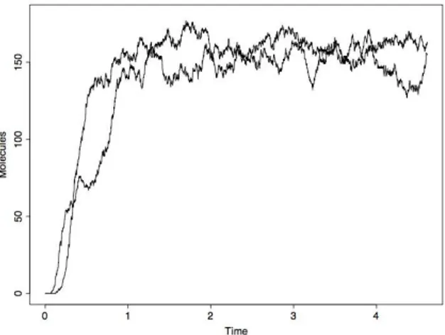
Figure 1 shows two time courses of the species M AP KP P from two
different simulated trajectories. The plots show the number of M AP KP P
(the effector species) molecules over time.
Figure 1: Two simulated trajectories of M AP KP P species in the MAPK
signaling cascade
Whereas a common trend can be identified in the two time courses, it is evident that the stochastic fluctuations make difficult to identify some of the salient features of the system, such as the time point at which it reaches a stationary state, or the exact stationary value for the number of M AP KP P
molecules. In the following section we will apply the ICA technique to extract from the n distinct trajectories this information together with a statistic characterization of the noise.
4.2 Application of ICA
As we stated before we consider the simulated time evolution of the number of M AP KP P molecules as the input for building the ICA model. In this
example we considered a number of n = 20 simulated time courses. We took this amount of trajectories as a compromise between different criteria:
variability of the trajectories, computational time required for the creation of them with the simulator, computational time and stability of results of ICA. Future investigations may be performed on the optimum number of simulated trajectories for the use of ICA. From the n trajectories we used ICA model estimation via FastICA algorithm looking for two components. The algorithm converges and the components returned, shown in Figure 2, display the main mode of behavior of the number of M AP KP P molecules,
and its stochastic fluctuations.
Figure 2: ICA results for the analysis of the M AP KP P simulated
trajecto-ries
The first component in Figure 2 can be easily interpreted. It shows the extent of the transient evolution of the system, the time point at which the system reaches a steady state (around time= 1) as well as the average value of the number of M AP KP P molecules at equilibrium (around 150).
The second component in Figure 2 describes the noise caused by the stochastic fluctuations. It exhibits higher variability during the transient phase, in correspondence to when the values of the simulated trajectories seem to show a higher variance (compare Figure 1).
Here, it is worthwhile mentioning that each of the n simulated input trajectories in the dataset contained K = 8000 samples, and that the com-putation of the two ICA components required about 3 seconds on a standard MacBook laptop equipped with 1GB of RAM.
It is important to notice that usually aggregated simulation trajecto-ries are described with their mean value and, as a measure of variation, with some kind of confidential intervals. Further analysis on the stochastic fluctuations are then neglected and the stochastic system reduced to its av-erage behavior. In contrast, the information returned by the ICA technique
through the second independent component allows, as we show in the next section, to obtain a more precise understanding of the stochastic fluctuations of biological systems, describing them in a statistical way.
4.3 A high-level statistical model of MAPK
In the previous section, ICA results on the evolution of the number of M AP KP P molecules has shown the possibility of describe it with two
com-ponents, the first one representing the main mode of behavior and the second one the stochastic fluctuations. Here we want to statistically characterize this latter component. To do so, we apply a statistical stochastic processes estimation technique.
From the global autocorrelation function and the partial autocorrelation function of the stochastic fluctuation component we derive a possible de-scription of the process as a first order autoregressive model [2], which using a standard notation will be denoted as AR(1). This type of model describes a process X at time t, Xt, as follows:
Xt= a + φXt−1+ εt (5)
where εt is a white noise process with zero mean and variance σ2, that is
εt∼ N (0, σ2). We fit such a kind of model on the data using the statistical
computing framework R. The estimated coefficients returned by the fitting are reported in Table 1.
Parameter Estimate a 0.0000 φ 0.9996
Table 1: AR(1) model parameter estimates
As expected, the estimate for a is zero, given that the second indepen-dent component for which it has estimated is a zero mean process. More-over, the parameter φ is very close to 1. It is useful recalling that AR(1) processes are stationary only if the parameter |φ| < 1. This proximity to 1 for the estimated parameter φ may be interpreted as the proximity to non-stationarity of the stochastic fluctuations. Goodness of fit is confirmed by residual analysis. They are normally distributed as the model hypothesis require.
Estimating an AR(1) model on the noise component of the system pro-vides a tool for describing the stochastic fluctuations, which can be further
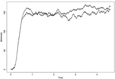
exploited to define a very simple and abstract model of the system. Indeed, realizations of the stochastic AR(1) model can be remixed, using the mixing weights obtained through ICA, with the first independent component, to simulate the number of M AP KP P molecules. Figure 3 shows two different
synthetic trajectories generated with the first resulting ICA component and two different simulated realizations of the fitted AR(1) model. As it can be observed, the synthetic trajectories in Figure 3 are very similar to the original ones reported in Figure 1.
Figure 3: Two trajectories from the reconstructed M AP KP P model
Therefore, with respect to the classical statistical analysis of simulation output, ICA has the advantage, at the expense of an additional computa-tional cost, of allowing a more complete characterization of the system in terms of both its main mode of behavior and its stochastic fluctuations. Such characterization allows also defining simple and easy to simulate stochastic models of the system.
5
Conclusions and future work
In this paper we investigated and we proposed the application of the In-dependent Component Analysis technique as an automated procedure to extract aggregate knowledge from a set of simulated trajectories obtained from stochastic simulation of biological models. ICA has been originally
proposed for signal analysis, but its generality allowed applications in var-ious other domains. Here, we showed that ICA can be effectively applied to the processing of noisy trajectories to obtain a characterization of both the main mode of behavior of the system and of the noise process. This processing can be easily automated thanks to the widespread availability of libraries implementing ICA.
We also showed that the knowledge obtained through the ICA technique can be used to build simple statistical abstractions that faithfully reproduce system behavior. These abstractions could be used to define computation-ally efficient models of systems that are easily amenable to inclusion in larger models.
We plan to extend the conceptual research results presented in this pa-per along a number of promising directions. First of all, we intend to extend and tailor the application of ICA to system exhibiting a dynamical equilib-rium, for instance biological oscillators such as Lotka-Volterra [22]. These systems pose several challenges to the analysis of their trajectories, which show stochastic fluctuations in both amplitudes and phases of the oscil-lations. Second, we want to investigate on the relationships between the decomposition returned by the ICA and the expected behavior of the sys-tem as estimated through the statistical averaging of multi-run trajectories. The smoothness of the first ICA component (the main mode of behavior) is clearly influenced by the amount of variability along the trajectories and this variability is reflected in the width of the confidence intervals obtained with statistical averaging. Finally, our plan is to build upon the simple statistical characterization of systems that can be defined from ICA results to tackle the study of the dynamics of complex systems were multiple instances of the same biochemical system are present, defining aproaches able to master the simulation computational cost for the overall model.
References
[1] C. Alexopoulos, Statistical analysis of simulation output: state of the art, in Proceedings of the 39th conference on Winter simulation, – WSC ’07, Washington D.C. USA, IEEE Press, pp. 150–161, 2007.
[2] G. E. P. Box, G. M. Jenkins, and G. C. Reinsel, Time series analysis: forecasting and control, Prentice Hall, New York, 1994.
[3] J.-F. Cardoso, Blind signal separation: statistical principles, Proceed-ings of the IEEE, 86(10):2009–2025, 1998.
[4] F. Ciocchetta, and J. Hillston, Bio-PEPA: An extension of the process algebra PEPA for biochemical networks, Electronic Notes in Theoretical Computer Science, 194(3):1571-0661, Elsevier Science Publishers B. V., Amsterdam, The Netherlands, 2008.
[5] P. Comon, Independent Component Analysis, a new concept ?, Sig-nal Processing, Elsevier, 36(3):287–314, 1994, Special issue on Higher-Order Statistics.
[6] T. Cover and J. Thomas, Elements of Information Theory, Wiley, 1991. [7] M. E. Davies, M. G. Jafari, S. A. Abdallah, E. Vincent, and M. D. Plumbley, Blind speech separation using space-time independent com-ponent analysis, in: S. Makino, T.W. Lee, and H. Sawada (Eds.), Blind Speech Separation, Springer, Dordrecht, The Netherlands, pp. 79–99, 2007.
[8] L. Dematt´e, C. Priami and A. Romanel, Modelling and simulation of biological processes in BlenX, SIGMETRICS Performance Evaluation Review, 35(4):32–39, 2008.
[9] D. T. Gillespie, A general method for numerically simulating the stochastic time evolution of coupled chemical reactions, Journal of Com-putational Physics, 22(4):403–434, 1976.
[10] D. T. Gillespie, Stochastic simulation of chemical kinetics, Annual Re-view of Physical Chemistry 58:35–55, 2007.
[11] A. Funahashi, N, Tanimura, M, Morohashi, and H. Kitano, CellDe-signer: a process diagram editor for gene-regulatory and biochemical networks, BIOSILICO, 1(5):159–162, 2003.
[12] A. Hyv¨arinen, Fast and robust fixed-point algorithms for Indepen-dent Component Analysis. IEEE Transactions on Neural Networks, 10(3):626–634, 1999.
[13] A. Hyv¨arinen, Independent Component Analysis: algorithms and ap-plications. Neural Networks, 13(4–5):411–430, 2000.
[14] S. Hoops, S. Sahle, R. Gauges, C. Lee, J. Pahle, N. Simus, M. Singhal, L. Xu, P. Mendes, and U. Kummer, COPASI - a COmplex PAthway SImulator, Bioinformatics, 22:3067–3074, 2006.
[15] C.-Y. F. Huang and J. E. Ferrell Jr, Ultrasensitivity in the mitogen-activated protein kinase cascade, Biochemistry, 93(19):10078–10083, 1996.
[16] S. Makeig, T.-P. Jung, A. J. Bell, D. Ghahremanis, and T. J. Sejnowski, Blind separation of auditory event-related brain responses into indepen-dent components, Proceedings of the National Academy of Sciences, USA, 94(20):10979–10984, 1997.
[17] T.-P. Jung, S. Makeig, T. Lee, M. McKeown, G. Brown, A. J. Bell, and T. J. Sejnowski, Independent component analysis of biomedical signals, in Proceedings of the 2nd International Workshop on ICA and BSS, June 19-22, Helsinki, Finland, pp. 633–644, 2000.
[18] P. Mendes, Biochemistry by numbers: simulation of biochemical path-ways with Gepasi 3, Trends in Biochemical Sciences 22(9):361–363, 1997.
[19] J. J. Murillo-Fuentes, Independent component analysis in the blind wa-termarking of digital images, Neurocomputing, 70(16-18): 2881–2890, Elsevier Science Publishers B. V., Amsterdam, The Netherlands, 2007. [20] M. Nagasaki, A. Doi, H. Matsuno and S. Miyano, Petri net based de-scription and modeling of biological pathways, in: H. Anai, and K. Horimoto, (Eds.), Computer Algebra in Biology, Universal Academy Press, Inc., Tokyo, pp. 19–31, 2005.
[21] S. Sedwards and T. Mazza, Cyto-Sim: A formal language model and stochastic simulator of membrane-enclosed biochemical processes, Bioinformatics, 23(20):2800–2802, 2007.
[22] V. Volterra, Variations and fluctuations of the number of individuals in animal species living together, Animal Ecology, McGraw-Hill, New York, pp. 409-448, 1931.
[23] P. D. Welch, The statistical analysis of simulation results, in: S. Laven-berg, (Ed.), The Computer Performance Modeling Handbook, pp. 268– 328, Academic Press, New York, 1983.