Italy’s ACE Tax and Its Effect on a Firm’s Leverage
Paolo Panteghini
University of Brescia, CESifo, AccounTax Lab
Maria Laura Parisi
University of Brescia
Francesca Pighetti
University of Brescia
Abstract This article describes the new ACE-type system implemented in Italy since
2012. The authors first show that this system reduces but does not eliminate the financial distortion due to interest deductibility. Using a dataset of Italian companies, the authors analyze the impact of this relief on Italian firm capital structure. Despite the permanence of a tax advantage and its gradual implementation, the ACE relief is estimated to reduce significantly leverage. By decreasing default risk it is also expected to reduce systemic risk.
JEL H25, H32
Keywords ACE; business taxation; leverage
Correspondence Maria Laura Parisi, University of Brescia, Italy. [email protected]
© Author(s) 2012. Licensed under a Creative Commons License - Attribution-NonCommercial 2.0 Germany Discussion Paper
1. 1. 1.
1. IntroductionIntroductionIntroductionIntroduction
On Monday, December 5th, 2011, the Italian Government presented a reform that aims not only to restore a balanced budget in 2013, but also to stimulate company capitalization, by means of the so-called “Aiuto alla Crescita Economica” (Aid to Economic Growth) instrument. This relief shares the acronym and the main characteristics of the British ACE.
Under both systems, the allowance is calculated by applying an imputation (or notional) rate to the equity invested into the company.1 Ordinary return, approximating the
opportunity cost of new equity capital, is exempt, while exceeding income is taxed at the corporate level. Therefore, by ensuring the deduction of the imputed income of equity capital, ACE reduces or even eliminates the tax advantage of debt finance, thereby encouraging firm capitalization.2
According to the Italian Government, ACE has two aims: 1) it is expected to boost Italy’s economic growth through a reduction of firm tax liabilities; 2) it is designed to enhance capital structure of Italian companies.3 It is worth noting that this provision is in line with
both the European Commission’s and the International Monetary Fund’s
recommendations, which stress the importance of implementing tax devices aimed at discouraging companies’ excessively high leverage and therefore, reducing systemic risk. In this article, we have first described the new ACE-type system and calculated the effective marginal tax rates (EMTRs) under full equity- and debt-finance. We then estimated the effect of this tax relief on firms’ leverage. To do so, we used a large and representative sample of Italian firms. Our preferred estimate of leverage elasticity to ACE is negative and statistically significant, equal to -0.064. This means that an overall increase in the benefit by 50% of the initial ACE benefit (such that the ACE/Sales ratio goes from 0.14% up to 0.21%) is estimated to change leverage by -3.2%, on average. Although this effect varies according to area, size and sectors, the ACE relief is in any case expected to
1
This tax provision is contained in a comprehensive fiscal reform aimed at reaching a balanced public budget in 2013. For further details on its characteristics and overall effects see, e.g., Arachi et al. (2012).
2 The idea of taxing above-normal income is not new: during the first world war, many countries
involved in that conflict introduced devices aimed at taxing "war-profiteering", that is profits that exceeded normal peace-time profits. See, e.g., Stamp (1917).
3
As stressed by the Government, Italian companies have a “relatively high” leverage (about 1.5, versus 0.6 in France and 0.7 in Spain, BACH data — industry trade). Moreover, they are subject to an effective tax rate which is well above the EU average (i.e., 27.4 percent against an EU average of 21.8 per cent, see EUROSTAT). According to Mr. Monti’s Government, therefore, the introduction of ACE will both reduce the tax burden and encourage a rebalancing of firm capital structure.
encourage company capitalization, therefore consistently reducing default risk. The reduction of systemic risk may be a necessary condition to reach the Government’s second target, i.e., boosting economic growth (the Achille’s heel of the Italian economy).
Section 2 of the paper describes the main characteristics of an ACE-type system and summarizes the international debate on this instrument. Section 3 provides a discussion of the Italian case, with reference to the main changes over the last decade. Section 4 discusses the econometric method and the estimation results. Section 5 reports some robustness checks of our results. Section 6 concludes.
2. ACE 2. ACE 2. ACE
2. ACE taxation throughout the worldtaxation throughout the worldtaxation throughout the worldtaxation throughout the world
According to the European Commission (2008), Italian firms are more exposed to debt than other European companies. Worry about this exposure has been voiced not only by
the European Commission, but also by the IMF (2009).4 Both institutions have shown that
this excessive debt exposure has been favoured by existing tax rules: by guaranteeing the (either partial or total) deductibility of interest on debt, many systems encourage debt finance, thus creating under-capitalization and raising default risk. To eliminate this distortion, both the IMF and the European Commission have illustrated various options. As such, the IMF analyzed certain mechanisms aimed at giving an incentive to self financing. Finally, it proposed the introduction of an Allowance for Corporate Equity (ACE) instrument, which had also been discussed previously by the Institute for Fiscal Studies (IFS, 1991).5 Similarly, in a report prepared for the European Commission in 2008,
a group of experts6 analyzed a few alternative proposals including:
• Introducing a mechanism similar to ACE;
4
The IMF report (2009) states: "Tax distortions are likely to have encouraged excessive leveraging and other problems evident in the financial market crisis. These effects have been little explored, but are potentially macro-relevant. Taxation can result, for example, in a net subsidy to borrowing of hundreds of basis points, raising debt-equity ratios and vulnerabilities from capital inflows" (p. 1). The IMF report also argues that: “Given the large potential macroeconomic damage from excess leverage, including balance of payment effects, it is hard to see why–as now is often the case– debt finance should be systematically tax-favoured” (p. 12).
5 According to the IFS proposal, the opportunity cost of finance should be equal to the default-free
interest rate, thereby making the Government "a sleeping partner in the risky project, sharing in the return, but also sharing some of the risk" (Devereux and Freeman, 1991, p. 8). Devereux and Freeman (1991) point out that, in present value terms, Brown (1948) cash-flow tax and the ACE tax are equivalent. This means that ACE does not distort investment decisions.
6
AAVV. (2008), Study on Effects of Tax Systems on the Retention of Earnings and the Increase of Own Equity, edited for the European Commission (Team Leader: Jean Albert; contract SI2.ICNPROCE009493100).
• Passing a law which would guarantee the benefits of using reinvested profits for a firm.
Even if these experts are doubtful about the effectiveness of ACE (as it has been used very rarely in real situations), they believe that solutions need to be found to stimulate the recapitalization of firms. As such, both the European Commission and the IMF agree about the problem of excessive corporate debt, while there are still differences of opinion about solutions to this problem.
It is worth noting that ACE-type systems had already been implemented in Croatia between 1994 and 2001 (see Keen and King, 2002). Moreover, dual tax systems were introduced not only in the Nordic countries and Italy but also in other countries, such as
Austria, Belgium and Brazil (see Eggert and Genser, 2005, Gérard, 2006, Klemm, 2006).7
Contrary to a cash-flow tax therefore, policy-makers aiming at implementing a dual tax system were able to rely on previous experience.
Recently, in an IMF working paper, De Mooij (2011) returned to this topic, pointing out that most countries guarantee a tax advantage for debt. He stated that this discrimination is becoming ever more difficult to justify, given the present state of affairs. In particular, he pointed out that the costs of this discriminatory treatment of financing sources “are larger, possibly much larger than we thought” (p. 3). For this reason, he proposed using ACE. He estimated that, if the benefits of ACE were applied to the whole net internal equity of largest countries, its cost would be about 0.5% of GNP. According to other authors (see, e.g., Griffith et al., 2010), he then proposed a gradual approach aimed at ensuring that ACE benefits only new wealth. This is exactly what happens with the Italian ACE.
3. The Italian ACE 3. The Italian ACE 3. The Italian ACE 3. The Italian ACE
The new ACE system shares some characteristics with the Italian Dual Income Tax (DIT), in force from 1998 to 2003. As shown in Box 1, under both regimes, profit is split into two components, i.e., ordinary and above-normal income. Unlike DIT, which taxed ordinary
income at a lower rate, ordinary income is exempt under ACE.8
7 See also Fehr and Wiegard (2003) and Keuschnigg and Dietz (2007), who proposed the
introduction of an ACE-type system in Germany and Switzerland, respectively. More recently, Griffith et al. (2010) have proposed the introduction of a dual income tax in the UK. They have also pointed out that if the British Government preferred to move “towards a consumption-based personal tax, the equivalent of such a system could be implemented by exempting the normal return to saving from tax at the personal level, just as the ACE allowance exempts the normal return at the corporate level” (p. 917).
8
Box 1: The Italian Dual Income Tax (1998-2003).
Under the Italian DIT, a gradual approach was implemented. Indeed, the favourable tax treatment involved only new subscriptions of capital and retained earnings, rather than the whole equity capital. The starting time was 1996, when the reform was originally presented by the Government. Thus the DIT benefit was nil at the beginning and increased over time as new subscriptions and retained earnings from 1996 onwards led to an accumulation of equity capital. In doing so, it ensured a "soft" move towards the final regime, under which all equity capital would have enjoyed DIT benefit. This gradual implementation was necessary to keep a close eye on public accounts, at a time when Italy was trying its best to gain access to the first stage of the European Monetary Union. For this reason, the average tax rate could not be less than 27%. As we pointed out, the Italian DIT tax was abolished in 2003. When the centre-right Government came to power in 2001, the attitude towards DIT radically changed. The imputation rate was almost immediately aligned to the rate of legal interest, and thus halved (declining from 6% to 3.5% first and then to 3%). Furthermore, only equity increases until June 30th, 2001 were relevant to calculate
the incentive. Cutting imputation rate and "freezing" the benefit were a clear signal of the future abandonment of the DIT, which occurred at the end of 2003.
Despite these limitations, related to the way it was designed and not to the instrument itself, its introduction had a significant effect. Bontempi et al. (2003) showed that, in a sample of about 12,000 companies, the debt/liability ratio was reduced on average by 0.21%. This result is particularly significant, because estimates were limited to the 1998-99 period. Similar results were also found in Bernasconi et al. (2005), who then urged policymakers to reconsider the elimination of the DIT system.
Under the ACE regime, the imputation rate used to calculate ordinary income is equal to 3%. Subsequently, it will be determined by the Minister of Economy and Finance (to be issued no later than January 31st of each year) and will be in line with the average return
of public bonds, increased by three percentage points.
As pointed out, the ACE benefit will be applied to new equity, the starting level being net wealth existing on December 31st, 2010 (which is the first year of application). If the
notional value of the ACE return exceeds the total amount of income, it will be deductible against income in the subsequent tax periods.9
In the first year of application, the ACE base is equal to the existing equity at the end of the previous year, less the profit earned during that year. This starting value is increased by the shareholders’ new cash contributions and retained profit. However, non-available
9Suppose for example that a company’s equity is 1 Million Euros in the current year: the
Ace relief will then be equal to 3 per cent of the equity times the existing corporate income tax rate (27,5 per cent), i.e., 0,275•(0,03•1.000.000) = 8.250 Euros. This relief can be either deducted from gross tax liability now (if it exceeds 8.250 Euros) or carried forward (if it is lower). If, for instance, gross tax liability is 5.250, the exceeding 3.000 Euros will be carried forward and deducted in future years.
reserves (e.g., due to the revaluation of a firm’s asset value) are not accounted for (see Box 2).10
It is worth noting that ACE applies not only to corporations but also to individual firms and limited partnerships. Although the treatment of individual firms and limited partnerships has to be ruled by a forthcoming decree of the Minister of Economy and Finance, the inclusion of all these kinds of business is an important measure, as it ensures neutrality in terms of organizational form.
Box 2: The Italian ACE (according to law 22 December 2011, n. 214 and Decree by the Ministry of Economy and Finance dated 14 March 2012).
The Ace base The Ace base The Ace base The Ace base
The increase of capital relevant to the facility comes from the algebraic sum of positive and negative elements. Positive elements are cash contributions (capital increases, payments to fund lost) and allocations of profit to reserves, except non-distributable reserves. The decree also assigns shareholders’ waiver of repayment of loans to positive items. Negative elements are voluntary distributions to shareholders (distribution of retained earnings, return of capital, allocation of assets) as well as some reductions due to anti-avoidance rules.
The ACE base besides includes profits allocated to the reserve profit used to cover losses or carried forward. In order to widen the Ace base, profit made in 2010 is also included. No surplus fund arising from differences on exchange rates are included.
Eligibility Eligibility Eligibility Eligibility
ACE is applied not only to corporations but also to sole proprietors and partnerships. However, this benefit is not granted to bankrupt firms; companies under either compulsory liquidation or extraordinary administration (this rule can be applied only to large companies).
Timing Timing Timing Timing
Contributions in cash detect since they are physically carried out. Therefore, in the year of payment, cash is considered according to a pro-rata basis criterion (i.e., if cash payments are
received July the 1st , only one half of it matters).
Anti Anti Anti
Anti----avoidance ruleavoidance ruleavoidance ruleavoidance rule
To avoid “cascade effects” if shareholders inject new equity in a company and this money is again transferred to a subsidiary, the contribution in cash at the hand of A is sterilized and the benefit is only guaranteed to B. By doing so, the law aims at eliminating the duplication of tax reliefs, especially in groups, against a single injection of capital or “refreshing” of the old capital with operations considered to be elusive (as intercompany purchases of companies).
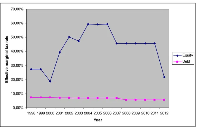
As already pointed out, the ACE relief is aimed at reducing or eliminating the tax advantage of debt. To show this, Figure 1 shows the dynamics of the effective marginal tax rate (EMTR) under both full equity- and debt-finance over the 1998-2012 period (calculations are available in Appendix 2). For simplicity, personal taxes are not considered. As can be seen, the EMTR under equity-finance shows a sharp increase, due to repealing DIT.
10
Similarly, equity is reduced in the event of: equity distribution, purchases of investment in subsidiaries, purchases of companies or business units.
In 2006 it went below 50% because of the corporate tax rate cut (from 33 to 27.5%). As can be seen, the introduction of ACE in 2012 led to a dramatic cut in EMTR. However, the tax advantage was reduced but not eliminated: this is due to the fact that the ACE imputation rate was now 3% namely, about one half of market interest rates.
Figure 1 — The effective marginal tax rate under equity and debt finance.
0,00% 10,00% 20,00% 30,00% 40,00% 50,00% 60,00% 70,00% 1998 1999 2000 2001 2002 2003 2004 2005 2006 2007 2008 2009 2010 2011 2012 Year E ff e c ti v e m a rg in a l ta x r a te Equity Debt
4. Estimated effects of the ACE relief 4. Estimated effects of the ACE relief 4. Estimated effects of the ACE relief 4. Estimated effects of the ACE relief
Due to budget constraints, the Italian Government decided not to extend this provision to the entire equity stock. According to Arachi et al. (2012), however, an ACE allowance proportional to the net wealth stock would have been affordable, as it would cost about 4 billion Euros (i.e., about 0.25% of GDP). In this case, the average effective tax rate would have been reduced by more than 9%.
Despite this gradual approach, we can expect that the EMTR cut would have a beneficial effect in terms of capitalization. In order to estimate this effect, we examined a sample of Italian firms, most of them being limited liability companies. There are 109,175 firms in the sample, about 10% of the overall limited-liability Italian firms, selected with a stratified method, which delivered a representative sample (see Appendix 1 for sample
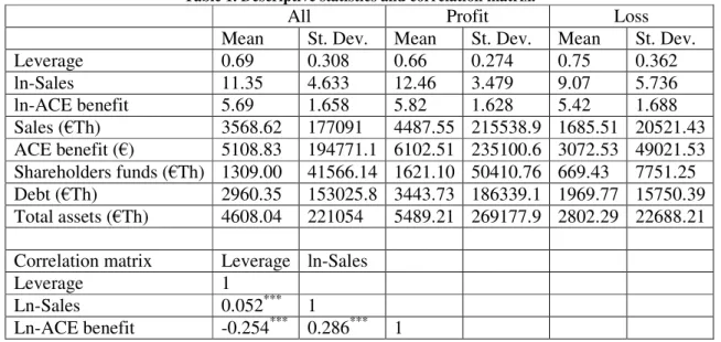
selection and description). Each firm is observed at least for two consecutive years over the time interval 2006-2010. Thus, the total number of observations is 445,857 (see Appendix 1). Table 1 shows some of the descriptive statistics of our sample. It is worth noting that firms differ in terms of size, shareholder funds and ACE benefit due to new equity injections. The correlation matrix of the main variables used in the regressions is also reported.
Table 1. Descriptive statistics and correlation matrix.
All Profit Loss
Mean St. Dev. Mean St. Dev. Mean St. Dev.
Leverage 0.69 0.308 0.66 0.274 0.75 0.362 ln-Sales 11.35 4.633 12.46 3.479 9.07 5.736 ln-ACE benefit 5.69 1.658 5.82 1.628 5.42 1.688 Sales (€Th) 3568.62 177091 4487.55 215538.9 1685.51 20521.43 ACE benefit (€) 5108.83 194771.1 6102.51 235100.6 3072.53 49021.53 Shareholders funds (€Th) 1309.00 41566.14 1621.10 50410.76 669.43 7751.25 Debt (€Th) 2960.35 153025.8 3443.73 186339.1 1969.77 15750.39 Total assets (€Th) 4608.04 221054 5489.21 269177.9 2802.29 22688.21
Correlation matrix Leverage ln-Sales
Leverage 1
Ln-Sales 0.052*** 1
Ln-ACE benefit -0.254*** 0.286*** 1
note: Sales are reported in thousand of euro. ACE benefit is reported in euro. Statistics are based on 445,857 observations for 109,175 firms over 5 years. Pair wise correlation coefficients are all statistically significant at 1% level.
The firms’ leverage is the ratio between the sum of current and non-current liabilities, over total assets.11 On average, it is 69% of total assets. Loss-making firms have a higher
leverage (75%) than profitable ones (66%), although the dispersion is higher. Not surprisingly, profit-making firms profited from a higher ACE benefit. As will be shown, however, for loss-making firms an increase in the ACE relief by an equal amount will ensure a greater benefit in terms of leverage decrease. Of course, ACE benefit, which ensures a cut in the effective tax ratio (tax liability on profit), frees up resources and according to the Government, could stimulate corporate activity.
In this article however, we have only focused on the first target, i.e., the expected decrease in leverage caused by ACE. To estimate this effect we opted for the following general (reduced) form equation:
it i it it it x ACE y =κ+β'~ +δ +α +ε , (1) 11
where the dependent variable yit is the leverage ratio.12 Index
i refers to the firms, t to year. ~ is a vector of firm variables, that is geographical position, size, sector of xit
production, or time-variant like age and whether reporting a profit/loss in the current year, i.e. I(EBIT>0)=1 for profit, I(EBIT>0)=0 for loss. Time dummies are included in all regressions. The variable ACE is the log of the ratio between ACE benefit and total assets; ACE benefit is calculated according to De Mooij (2011) by considering that loss-making firms enjoy a lower benefit due to carry forward devices. This reduces the ACE benefit for loss-making firms by 50%. Details are provided in Table 2. Finally, αi represents all other unobservable individual effects, and εit is an idiosyncratic error term, assumed uncorrelated with the unobserved and observed characteristics.13
Table 2. ACE benefit formula
Profitable firms 0,275*i*base ACE
Loss-making firms 0,5*0,275*i*base ACE
note: 0.275 is the statutory corporate income tax rate; i is the imputation rate; the ACE base is equal to the increase in net wealth observed since 2010.
In our regressions, we use both Fixed Effects and pooled-OLS (as well as random effects for a specification test) types of estimator, given that pure OLS should be upward biased if fixed effects are present in the sample and positively correlated with the other characteristics, or downward biased otherwise.14 Pooled-OLS allowed us to condition the
elasticity estimates on various firm fixed characteristics (i.e., location, size, sector) plus a set of interaction terms between the ACE variable and fixed characteristics, useful to run a Wald test of parameter stability, as illustrated in Table 3, column 4. Within-group Fixed Effects estimator allowed us to take care of any potential fixed effect correlation with the explanatory variables x~ , but it canceled out time-invariant characteristics. To estimate it the elasticity of leverage to ACE in the sub-populations with same characteristics, we need to apply the within-group estimator to sub-samples (Table 3, column 2). Notice that the dummy I(EBIT>0) changes over time; however in order to define the subpopulation of profitable firms (and losing profit firms), we decided to build two groups in the following
12
Bernasconi, Marenzi, Pagani (2005), Miniaci, Panteghini, Parisi (2012), Gurcharan (2010), among others, use similar reduced-form approaches in the estimates. See also note 17.
13
We will alternatively use the Fixed Effects within-group estimation method and the Random Effects method, and run a Hausman test of specification. In the Random Effects method, we also drop the assumption of independence between
α and x, and correct for this bias (see Wooldridge, 2002). We furthermore run tests of autocorrelation for the error term
in order to exclude dynamic mechanisms in the leverage.
14
As clear from Table 3, this is always the case in the Leverage equation for few subpopulations, i.e. North East, Small, Profit, Loss, where the OLS estimates are upward biased. Notice that the coefficient of ln-ACE benefit is negative.
way: if a firm showed positive EBIT in 2008 then it enters the sub-population “Profit”, otherwise it enters the subpopulation “Loss”.15 The former enjoys the whole benefit
whereas the latter has a 50% reduction in ACE relief.
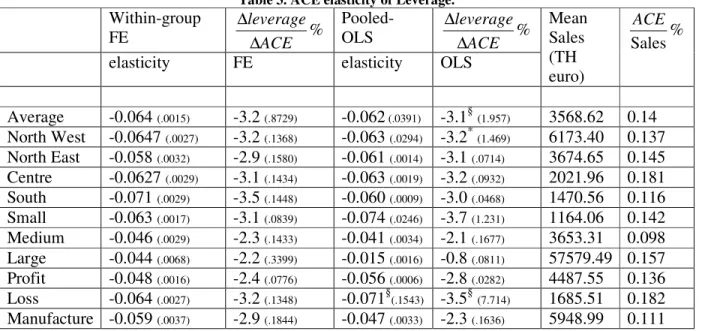
Table 3. ACE elasticity of Leverage. Within-group FE ACE % leverage ∆ ∆ Pooled-OLS ACE % leverage ∆ ∆
elasticity FE elasticity OLS
Mean Sales (TH euro) % Sales ACE Average -0.064 (.0015) -3.2 (.8729) -0.062(.0391) -3.1§(1.957) 3568.62 0.14 North West -0.0647 (.0027) -3.2 (.1368) -0.063 (.0294) -3.2*(1.469) 6173.40 0.137 North East -0.058 (.0032) -2.9 (.1580) -0.061 (.0014) -3.1 (.0714) 3674.65 0.145 Centre -0.0627 (.0029) -3.1 (.1434) -0.063 (.0019) -3.2 (.0932) 2021.96 0.181 South -0.071 (.0029) -3.5 (.1448) -0.060 (.0009) -3.0 (.0468) 1470.56 0.116 Small -0.063 (.0017) -3.1 (.0839) -0.074 (.0246) -3.7 (1.231) 1164.06 0.142 Medium -0.046 (.0029) -2.3 (.1433) -0.041 (.0034) -2.1 (.1677) 3653.31 0.098 Large -0.044 (.0068) -2.2 (.3399) -0.015 (.0016) -0.8 (.0811) 57579.49 0.157 Profit -0.048 (.0016) -2.4 (.0776) -0.056 (.0006) -2.8 (.0282) 4487.55 0.136 Loss -0.064 (.0027) -3.2 (.1348) -0.071§(.1543) -3.5§(7.714) 1685.51 0.182 Manufacture -0.059 (.0037) -2.9 (.1844) -0.047 (.0033) -2.3 (.1636) 5948.99 0.111
note: Robust standard errors in parentheses. All estimations are statistically significant at 1% level. Loss/Profit refer to 2008: if a firm profit is positive in 2008, then it is considered profitable all its time span. ∆ACE is the ACE change such that ACE/Sales ratio increases by 50%. Sales are reported in thousand euro and are averaged across years and firms overall and within each category. ACE/Sales is average ACE over average Sales. Based on 445857 observations. § indicates non significant.
Table 3 reports estimates of the elasticity of leverage with respect to ACE. To give an idea of the characteristics of each sub-group considered, the last two columns of Table 3 report the within-group average Sales in thousand of euro and the ratio between the ACE benefit and sales.
Column 2 shows the FE estimates of leverage elasticity: there is a negative statistically significant relation between the two variables as expected, and the relation is stronger for North-Western and Southern firms, small and loss-making firms. Column 4 reports the analogous Pooled-OLS estimates, which are quite close, even if with larger standard errors, on average.16 Indeed, Pooled-OLS estimate for Losing-profit firms is non significant.
15
In 2008 there are 177310 firms in the sample: 61.65% show positive EBIT in the balance sheet, 38.35% have negative or null EBIT. So we use the dummy I(EBIT>0) varying over time and firms as a regressor, while we use
I(EBIT>0)2008 as a criterion to define the subpopulations ‘Profit’ and ‘Loss’. For those firms observed only in the two
years 2006-2007 and 2009-2010, we applied the information about positive/negative profit in 2007 and 2009, respectively, given that they are the closest years to our benchmark year.
16
This means that on average unobserved fixed effects are not correlated to explanatory variables. Some distortion however is evident for South sub-sample, Small and Large firms, Profitable and Manufacturing. See note 14.
In column 3 we calculated the effect of a change in ACE benefit from its initial base on the leverage change. We considered a 50% ACE increase such that the ACE/Sales ratio steps from 0.14% to 0.21%. As can be seen, the lowest ratio is in the Medium firms sub-sample (0.098%), while the highest ratio belongs to firms in the Centre category and to firms with earnings loss (0.18%). When applying that increase for all sub-groups, we obtain the results on the leverage change, in percentage points, reported in columns 3 and 5. A recapitalization aimed at increasing the ACE benefit by 50% is estimated to reduce leverage by 3.2% overall. The impact is slightly larger in the South of the country (-3.5%). Small firms reduce leverage more than medium and large ones (-3.1%). Loss-making firms reduce leverage by 3.2%, whereas profitable firms have a 2.4% decrease. As is clear from Table 3, profitable firms show a lower elasticity of leverage than non-profitable firms in absolute value, -0.048 and -0.064 respectively, even if OLS estimate for losing firms is not statistically significant. This means that, if resources are available, the ACE benefit can stimulate loss-making firms more than it does for profitable firms. On aggregate, this would improve credit market conditions and, as expected by the IMF, reduce systemic risk.
5. Robustness checks 5. Robustness checks 5. Robustness checks 5. Robustness checks
The vast empirical literature on - the more general - relations between leverage and non-debt tax shields uses different specifications.17 For this reason, we needed to run some
robustness checks by changing the specification or the estimator in leverage equation (1). In particular we added a set of alternative explanatory variables to eq.(1), for the entire sample: size dummies, ln-Sales, “others” including the level of tangible fixed assets (over total fixed assets), the level of intangible fixed assets (over total fixed assets), the level of EBIT (over total fixed assets), the ratio of inventories to total fixed assets and age.
Within-group Fixed Effect elasticities are reported in Table 4, column 4. Last column of Table 4 shows the change in leverage due to a change in ACE, as before. When we substitute ln-Sales to size dummies, the estimated elasticity is only slightly higher in absolute value -0.067. This led to a reduction in leverage by 3.4%. Changing variables in the specification did not have any significant impact on calculation of elasticities through the FE method. However, adding ln-Sales to Pooled-OLS estimations does change the estimates, which are upward biased. It is very probable that current individual fixed effects are highly correlated with current sales, as discussed in the previous section. As a
17
Besides the papers cited in note 12, we mention, among others, Teker et al. 2009, Kahle and Shastri, 2005, Manuel and Pilotte, 1992. All these empirical work use a reduced-form approach.
consequence, we proceeded with a second robustness check, by finding instruments for sales. We needed to estimate equation (1) by GMM, where Leverage is the dependent variable and ln-Sales becomes endogenous (instrumented by lagged ln(Tornqvist index), lagged ln(Labor), ln-ACE, area and sector dummies). We also added the set of other variables explained above plus age in the main equation. The results for GMM are reported in the last panel of Table 4.
Table 4. Robustness checks for the leverage equation.
Added Variables Obs Elasticity
Estimation
Method ACEbenefit
leverage ∆ ∆ % SD 437194 -0.064 (0.0015) -3.2 (0.0729) lnS 437194 -0.067 (0.0014) -3.4 (0.0724) SD+others 437094 -0.064 (0.0015) -3.2 (0.0729) lnS+others 437094 -0.068 (0.0015) -3.4 (0.0726) SD+others+Age 435180 -0.062 (0.0014) -3.1 (0.0694) Fixed effects lnS+others+Age 435180 -0.066 (0.0014) -3.3 (0.0691) SD 437194 -0.063 (0.0391) -3.1 (1.957) lnS 437194 -0.082 (0.0049) -4.1 (0.2436) SD+others 437094 -0.064 (0.0005) -3.2 (0.0240) lnS+others 437094 -0.088§(1.399) -4.4§(69.594) SD+others+Age 435180 -0.054 (0.0005) -2.7 (0.0249) Pooled-OLS lnS+others+Age 435180 -0.072 (0.0020) -3.6 (0.1001) GMM lnS 250872 -0.063 (0.0019) -3.1 (0.0974) lnS+others 250832 -0.062 (0.0019) -3.1 (0.0971) lnS+others+Age 249742 -0.062 (0.0020) -3.1 (0.0977)
note: All regressions contain area, profit, sector and time dummies. Other variables are added alternatively: SD = Size dummies, lnS = ln(Sales), Age, others (Total Tangible Assets/Total Assets, Total Intangible Assets/Total Assets, Inventories/Total Assets, EBIT/Total Assets). 2-step robust GMM is applied in the last panel: instruments are ln(ACE benefit), lagged ln(Tornqvist index of raw materials + services), lagged ln(Labor), and all common factors. Hansen J statistic of over identification cannot reject the null in all three cases (J = 0.10, p-val. 0.748 first case; J = 0.07, p-val. 0.798 second case; J = 0.16, p-val. 0.689 third case). § indicates not significantly different from zero.
Now, after instrumenting sales, Leverage elasticity to ACE benefit estimated by GMM is not significantly different from its FE equivalent. Indeed, the two methods provide very similar calculated impacts of an ACE increase on Leverage decrease (see the last column). The ACE/Sales ratio increase corresponds, as in Table 3, to 50% of its initial value. This
would reduce leverage by -3.1%, according to our preferred FE and GMM measures.18
18
We think that our preferred estimates are the within-group FE estimates of Table 3 as far as Leverage is concerned, as discussed above, which are robust to changes in specification or estimation method. Adding a new dynamic equation for
6. Conclusion
Italy’s ACE is expected to reduce the tax advantage of debt-finance and thus encourage corporate capitalization. Using a large and representative sample of Italian firms, we have shown that, on average, the elasticity of leverage to the introduction of an ACE benefit would be -0.064, according to our preferred FE estimation method. If firms decided to inject further equity to increase the ratio between the ACE benefit and sales, say by 50%, the mean leverage would be reduced by 3.2%. Nonetheless both elasticity and the impact of an ACE change on leverage depend on location, size, health status, and sectors in which firms operate.
Moreover, our data indicate that the ACE benefit would lead a firm to decrease its tax burden by 18% to 20%, focusing on the 2007 and 2009 balance sheets, respectively. We can therefore say that, despite its gradual implementation, ACE is a step in the right direction, as it encourages firms to reduce leverage and therefore cut systemic risk. According to the Government, this may be a necessary condition for a higher growth rate in Italy’s economy.
sales (as we tried separately) cannot give further evidence of an indirect effect of an ACE relief on Leverage passing through Sales (the estimated impact of ACE on leverage does not change respect to our preferred one-equation results).
References References References References
Arachi G., Bucci V., Longobardi E., Panteghini P.M., Parisi M.L., Pellegrino S., and A. Zanardi (2012): “Fiscal Reforms during Fiscal Consolidation: The Case of Italy”, CESifo W.P. 3753.
Bernasconi M., Marenzi A. and L. Pagani (2005): “Corporate Financing Decisions and Non-Debt Tax Shields: Evidence from Italian Experiences in the 1990s”,
International Tax and Public Finance, vol. 12, pp. 741-773.
Bond S.R. and M.P. Devereux (1995): “On the Design of a Neutral Business Tax under Uncertainty”, Journal of Public Economics, vol. 58, pp. 57-71.
Bond S.R. and L. Chennells (2000): Corporate Income Taxes and Investment: A Comparative Study, London, Institute for Fiscal Studies.
Bontempi E., S. Giannini and R. Golinelli (2003): “Corporate Taxation and Its Reforms: Effects on Corporate Financing Decisions in Italy”, SIEP, October.
Bordignon M., S. Giannini and P.M. Panteghini (1999), “Corporate Taxation in Italy: The 1998 Reform”, FinanzArchiv, vol. 56, n. 3/4.
– (2001): “Reforming Business Taxation: Lessons from Italy?”, International Tax and
Public Finance, vol. 8(2), pp. 191-210.
Brown E.C. (1948): Business-Income Taxation and Investment Incentives, in L.A. Meltzer, E.D.
De Mooij Ruud A. (2011): “Tax Biases to Debt Finance: Assessing the Problem, Finding Solutions”, International Monetary Fund, Fiscal Affairs Department, May 3.
Devereux M.P. and H. Freeman (1991): “A General Neutral Profits Tax”, Fiscal Studies,
vol. 12, pp. 1-15.
Devereux M.P. and R. Griffith (1999): “The Taxation of Discrete Investment Choices”, IFS Working Papers, W98/16.
Domar et al. (eds.), Income, Employment and Public Policy, Essays in Honour of A.H. Hansen, W.W. Norton & c., New York.
European Commission (2008): “Study on Effects Of Tax Systems On The Retention Of Earnings And The Increase Of Own Equity”, Team leader: Jean Albert, Contract Si2.Icnproce009493100, Sept., Bruxelles.
Eggert W. and B. Genser (2005): “Dual Income Taxation in EU Member Countries”,
CESifo DICE Report, 1/2005, pp. 41-47.
Fehr H. and W. Wiegard (2003): ACE for Germany? Fighting for a Better Tax System, in M. Ahlheim, H.D. Wenzel and W. Wiegard, Steuerpolitik - Von der Teorie zur Praxis, Festschrift für Manfred Rose, Springer-Verlag, Berlin.
Gérard M. (2006): “Belgium Moves to Dual Allowance for Corporate Equity”, European
Taxation, vol. 4, pp. 156—62.
Griffith R., Hines J. and P.B. Sørensen (2010): International Capital Taxation, in J. Mirrlees, S. Adam, T. Besley, R. Blundell, S. Bond, R. Chote, M. Gammie, P. Johnson, G. Myles and J. Poterba (eds), Dimensions of Tax Design: the Mirrlees Review, Oxford University Press, Oxford.
Gurcharan S. (2010): “A Review of Optimal Capital Structure Determinant of Selected
ASEAN Countries”, International Research Journal of Finance and Economics, vol.
47, pp. 32-44.
Khale K.M. and K. Shastri (2005): “Firm Performance, Capital Structure, and the Tax
Benefits of Employee Stock Options”, Journal of Financial and Quantitative
Analysis, vol. 40(1), March, pp. 135-160.
Keen M. and J. King (2002): “The Croatian Profit Tax: An ACE in Practice”, Fiscal
Keuschnigg C. and M. Dietz (2007): “A growth oriented dual income tax”, International Tax and Public Finance, Springer, vol. 14(2), pp. 191-221, April.
Klemm A. (2006): “Allowances for Corporate Equity in Practice”, IMF Working Paper No. 06/259.
IFS Capital Taxes Group (1991): “Equity For Companies: A Corporation Tax For The 1990s”, A Report Of The IFS Capital Taxes Group Chaired By M. Gammie, The Institute For Fiscal Studies, Commentary 26, London.
IMF (2009): “Debt Bias and Other Distortions: Crisis-Related Issues in Tax Policy”, Fiscal Affairs Department, June
Manuel T. and E. Pilotte (1992): “Production Technology, Nondebt Tax Shields, and Financial Leverage”, Journal of Financial Research, vol. XV(2), pp. 167-180.
Miniaci R., P.M. Panteghini, M.L. Parisi (2012): “Debt Shifting in Europe”, mimeo
Panteghini P.M. (2001): “Dual Income Taxation: The Choice of the Imputed Rate of Return”, Finnish Economic Papers, vol. 14, pp. 5-13.
Panteghini P.M. (2006): “S-Based Taxation under Default Risk”, Journal of Public
Economics, vol. 90, pp. 1923-1937.
Sørensen P.B. (2005a): “Neutral Taxation of Shareholder Income”, International Tax and
Public Finance, vol. 12, pp. 777-801.
Sørensen P.B. (2005b): “Dual Income Taxation: Why and Now?”, FinanzArchiv, vol. 61,
pp. 559-586.
Sørensen P.B. (2007): “Can Capital Income Taxes Survive? And Should They?”, CESifo Economic Studies, vol. 53, pp. 172-228.
Stamp J.C. (1917): “The Taxation of Excess Profits Abroad”, Economic Journal, vol. 27,
pp. 26-37.
Teker D., Tasseven O. and A. Tukel (2009): “Determinants of Capital Structure for
Turkish Firms: A Panel Data Analysis”, International Research Journal of Finance
and Economics, vol. 29, pp. 179-187.
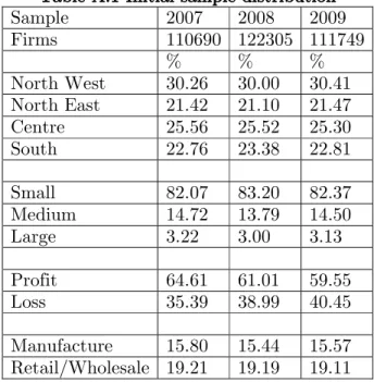
Appendix 1: Sample selection. Appendix 1: Sample selection. Appendix 1: Sample selection. Appendix 1: Sample selection.
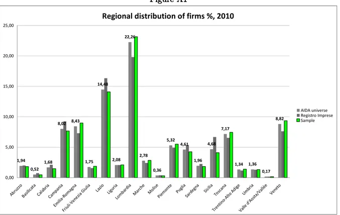
We based our simulation exercise on balance sheets and financial statements of Italian firms collected in the AIDA database, by Bureau van Dijk. As of October 20, 2011 (the time in which we downloaded the balance sheets) updated information was available for 1,215,703 firms. We deleted those firms which did not claim their Italian ATECO 2007 activity code (2-digit), Region of legal residence or their 2008 Total Value of Production and as a consequence, the AIDA universe reduced to 816,934 firms. We selected 15% of the universe firms with a stratified method, based on geographical location, activity sectors and size. The size of our sample was 122,313 companies, observed over the period 2006-2010, an unbalanced panel. Figure A1 illustrates the geographical distribution of firm frequency (only for limited liability companies, which make the most of the universe) of the AIDA universe (grey), the extracted sample (green) and the firms listed on the
Registro Imprese in 2010, the formal register of the Union of Chambers of Commerce (black). We compared our sample distribution with that of Registro Imprese which is an external source of information, independent of the Bureau van Dijk. While AIDA database tends to slightly over-represent Northern regions and Registro Imprese tends to over-represent Southern regions, our sample by construction mimics AIDA. The differences however were quite marginal and on average the sample satisfactorily represented the Italian industrial structure. More than one fifth of the firms are in Lombardy, 15% in Lazio, within the capital area, 9% in Veneto, relatively the most industrialized regions in Italy as expected. Our sample contains fewer firms with different legal forms, such as cooperatives, consortia, etc.. For those small groups we obtained good representation of
their Registro Imprese counterpart, as well. Unfortunately, we did not have any access to
Turnover or Total Value of Production of the firms in the Registro Imprese, in order to be able to check for size representativeness of our sample.
Figure A Figure A Figure A Figure A1111
Regional distribution of firms %, 2010
1,94 0,52 1,68 8,02 8,43 1,75 14,48 2,08 22,26 2,78 0,36 5,32 4,61 1,96 4,68 7,17 1,34 1,36 0,17 8,82 0,00 5,00 10,00 15,00 20,00 25,00 Abru zzo Basil icat a Cala bria Cam pani a Em ili a-Rom agna Friu li-Ve nezia Giu lia Lazio Ligur ia Lom bard ia Mar che Mol ise Piem onte Puglia Sard egna Sicilia Tosc ana Tren tin o-Alto Adi ge Um bria Valle d'A osta /Val lée Vene to AIDA universe Registro Imprese Sample
Table A.1 Table A.1 Table A.1
Table A.1 Initial sInitial sInitial sample distributionInitial sample distributionample distribution ample distribution
Sample 2007 2008 2009 Firms 110690 122305 111749 % % % North West 30.26 30.00 30.41 North East 21.42 21.10 21.47 Centre 25.56 25.52 25.30 South 22.76 23.38 22.81 Small 82.07 83.20 82.37 Medium 14.72 13.79 14.50 Large 3.22 3.00 3.13 Profit 64.61 61.01 59.55 Loss 35.39 38.99 40.45 Manufacture 15.80 15.44 15.57 Retail/Wholesale 19.21 19.19 19.11
We further proceeded to eliminate those firms whose balance sheets did not allow us to calculate their leverage, or those with missing current sales (2,526 firms). We eliminated 1,265 firms with just one observation in time (1,260 in 2008 and 5 in 2010), and another 1,081 observations for missing sales. To avoid outliers, we eliminated extreme leverage observations, outside 1-99 percentiles of the distribution (9813 observations). We finally eliminated the extreme values of ACE benefit. We ended up with 445,857 total observations for 109,175 firms. ACE variable has 437,194 observations and Age was observed in 443,907 cases.
Appendix 2: The calculation of the Appendix 2: The calculation of the Appendix 2: The calculation of the
Appendix 2: The calculation of the EMTR EMTR EMTR EMTR....
DIT (1998-2003)
For the Italian DIT, two regimes were considered: the one immediately after the 1998 tax reform and the final one. Under the Italian DIT indeed, the favourable tax treatment involved only new subscriptions of capital and retained earnings, rather than the whole equity capital. The starting point was 1996, when the reform was originally presented by the Government. Thus the DIT benefit was nil at the beginning and increased over time as new subscriptions and retained earnings from 1996 onwards led to an accumulation of equity capital. In doing so, it ensured a "soft" move towards the final regime, under which all equity capital would have enjoyed DIT benefit. This gradual implementation was necessary to keep a close eye on public accounts, at a time when Italy was trying its best to gain access to the first stage of the European Monetary Union. For this reason, the average tax rate could not be less than 27%.
The Government was conscious that DIT would have produced significant benefits only in the medium term. Furthermore, it was aware that this mechanism would have guaranteed a benefit only to under-capitalized firms, in the event that they rebalanced their debt/equity structure. Moreover, the rules encouraged new business initiatives, which would fully enjoy DIT relief. In order to enhance DIT relief, a corrective measure, called as Super-DIT, was introduced in the year 2000: the increase in capital invested was
multiplied by 1.2 in 2000 and 1.4 in the subsequent fiscal years, thereby boosting the DIT benefit proportionally.
As we pointed out, the Italian DIT tax was repealed in 2003. When the centre-right Government came to power in 2001, the attitude towards DIT radically changed. The imputation rate was almost immediately aligned to the rate of legal interest, and thus halved (declining from 7% to 3.5% first and then to 3%). Furthermore, only equity increases until 30th June 2001 were relevant to calculate the incentive, and the Super-DIT multiplier was removed. The cut in the imputation rate and the "freezing" of the benefit were a clear signal of the future abandonment of the DIT, which occurred at the end of 2003. IRAP (1998) IRAP (1998) IRAP (1998) IRAP (1998)
IRAP is a flat-rate tax levied on the value added generated by all types of business and self-employed activities. The tax base is calculated annually from taxpayers’ accounts according to a direct subtraction method. Value added is specifically defined for the different categories of taxpayers, depending on the type of business activity carried out. Specific rules, for example, are established for banks, financial intermediaries and insurance companies.
Apart from these exceptions, most other business activities have their tax base calculated as the accounting difference between sales revenue and the costs of intermediate goods and services. Neither labour costs nor interest payments are deductible from the tax base. Thus, the IRAP tax base is essentially equal to the sum of wages, profits, rents and interest payments at the business level. Outlays for capital goods are not immediately expensed, but taxpayers may deduct fiscal depreciation allowances from the tax base, including accelerated depreciation during the first three years. IRAP may thus be defined as a tax on value added of the net income variety.
Initially, IRAP rate was equal to 4.25%. In 2008 it was reduced to 3.9%. Moreover, in 2009, 10% of IRAP liability was deductible against IRES for companies with passive interest payments or personal costs.
EMTR EMTR EMTR EMTR
In order to analyze the impact of Italian taxation reforms, we proposed the EMTR values for Italian companies from 1998 to 2012. We considered a company that finances one project by debt or equity. The focus of this paper is only the holding-company taxation and not dividend taxation weighting down shareholders, so it is possible not to consider personal taxation, because of the multiplicity of variables related to it.
According to Bond and Chennells (2000), only capital has been considered and not the labor factor. Moreover capital does not depreciate during the time. In order to define the effective marginal tax rate (EMTR), we used the traditional standard methodology proposed by Devereux and Griffith (1999) and the linked studies of Bond and Chennells (2000).
We have assumed that a project is financed alternatively by equity or debt. The project invests one unit of capital, that can generate future profits, but that cannot depreciate over time.
1 11
1 Fully equityFully equityFully equityFully equity----financed investment financed investment financed investment financed investment
The first situation is about a company that finances the investment by equity and so the related future profits will be obtained through future dividends. Let’s define π as the marginal product of capital, i the market interest rate, τ the corporate income tax rate, tr the IRAP rate, and R the user cost of capital.
In the standard Italian situation, without DIT or ACE, the user cost of capital is derived from the following equation that equalize the net dividend on capital marginal unit to the opportunity cost without personal taxation:
. i r = − −πτ πτ π
The LHS measures the after-tax marginal product of capital, whereas the RHS is equal to the (marginal) opportunity cost of capital (i.e., i). Rearranging thus gives:
, 1 R i r = − − = τ τ π
where R is the user cost of capital under full equity finance.
In order to consider DIT and Super-DIT treatment, we define ρ as the imputed return on equity, m the Super-DIT multiplier, and t the reduced capital income tax rate. The user cost of capital is defined from this equation:
, ) ( m i tm − − − r = − ρ τ π ρ πτ π
which can be rewritten as follows:
R t m i r = − − − − = τ τ τ ρ π 1 ) (
Since 2012, an ACE-type relief has been coming into force. Defining e as the ACE imputation rate, the user cost of capital is equal to
i e
r − − =
−πτ τ(π ) π
Rearranging thus gives:
. 1 R e i r = − − − = τ τ τ π
As can be seen, even if e = i, a distortion arises due to IRAP (see Bordignon et al. 1999). 2
22
2 Fully debtFully debtFully debtFully debt----financed investment financed investment financed investment financed investment
In order to define cost of capital related to investment financed by equity, we have considered the same project analyzed in the previous paragraph.
Now the project is financed by debt, so company will return capital and related interests. In this scenario, we calculate the after-tax return under debt finance. Since there are no opportunity costs we thus obtain: π −i−πτr −τ(π−i)=0. Solving for π gives the user cost of capital (LHS) R i r = − − − = ) 1 ( ) 1 ( τ τ τ π
This formula holds until 2008. Since 2009, 10% of IRAP tax liability due to borrowing is deductible from the IRES base. Therefore, the after-tax marginal product of capital is equal to , 0 ) 1 . 0 ( − − = − − −i πτr τ π i πτr π
where 0.1τrπ is the IRES tax benefit arising from the partial deductibility of IRAP tax burden.
Rearranging one obtains:
R i r r = + − − − = τ τ τ τ τ π 1 . 0 1 ) 1 ( 3 33
3 The EMTRsThe EMTRsThe EMTRsThe EMTRs
Over the 1998-2012 period the Italian system has been modified several times. For this reason, in Table A2, we report the relevant parameters regarding both the DIT and the ACE system. In Table A3, we calculate the EMTR series, under either full equity- and debt-finance.
Table A.2: Italy’s tax parameters
DIT Tax rates
Year reduced capital income tax rate Super-DIT multiplier imputed return on equity Corporate income tax rate IRAP tax rate 1998 19,00% 1 7,00% 37% 4,25% 1999 19,00% 1 7,00% 37% 4,25% 2000 19,00% 1,2 7,00% 37% 4,25% 2001 19,00% 1,4 3,50% 36% 4,25% 2002 19,00% 1 3,00% 36% 4,25% 2003 19,00% 1 3,00% 34% 4,25% 2004 33% 4,25% 2005 33% 4,25% 2006 33% 4,25% 2007 33% 4,25% 2008 27,50% 3,90% 2009 27,50% 3,90% 2010 27,50% 3,90% 2011 27,50% 3,90% 2012 27,50% 3,90%
Table A.3: EMTR values, under either fully equity- or debt-finance. EQUITY
EQUITY EQUITY
EQUITY DEBTDEBT DEBTDEBT
Year EMTR Treatment Year EMTR Treatment
1998 27,32% DIT 1998 7,23% Standard** 1999 27,32% DIT 1999 7,23% Standard* 2000 18,74% DIT 2000 7,23% Standard* 2001 39,48% DIT 2001 7,11% Standard* 2002 50,29% DIT 2002 7,11% Standard* 2003 47,37% DIT 2003 6,88% Standard* 2004 59,36% Standard* 2004 6,77% Standard* 2005 59,36% Standard* 2005 6,77% Standard* 2006 59,36% Standard* 2006 6,77% Standard* 2007 59,36% Standard* 2007 6,77% Standard* 2008 45,77% Standard* 2008 5,69% Standard* 2009 45,77% Standard* 2009 5,52% 10% IRAP** 2010 45,77% Standard* 2010 5,52% 10% IRAP** 2011 45,77% Standard* 2011 5,52% 10% IRAP** 2012 21,72% ACE 2012 5,52% 10% IRAP**
* Standard means that a standard corporate income tax (named IRES since 2004) is applied.
Please note:
You are most sincerely encouraged to participate in the open assessment of this discussion paper. You can do so by either recommending the paper or by posting your comments.
Please go to:
http://www.economics-ejournal.org/economics/discussionpapers/2012-31
The Editor