ANSYS® Fluent simulation of a conventional chimney

MASTER FINAL PROJECT

MASTER OF ENVIRONMENTAL ENGINEERING

ANSYS® Fluent simulation of a

conventional chimney

Author

Roger Pitarch Gres

June 2019

Director/s

Dr. Ricard Torres Castillo

Dra. Alexandra Elena Bonet Ruiz

Department of Chemical Engineering and Analytical

Chemistry. Departmental Section of Chemical

Engineering. University of Barcelona

Agraïments

Primer de tot vull agrair la col·laboració de totes aquelles persones que han fet possible la realització d’aquest treball.

Per començar, vull agrair als meus tutors, la Dra. Alexandra Bonet i el Dr. Ricard Torres, la oportunitat que em va brindar de formar part d’aquest projecte, la seva ajuda, els seus clarificadors comentaris i la seva dedicació. Ha estat la meva primera experiència en el món de la simulació i realment, puc afirmar que és un camp força complex a la vegada que interessant.

També vull agrair a la meva família el seu suport moral en tot moment, especialment el dels meus pares.

I, per últim, vull agrair-li a la meva amiga Eva Martínez que hagi aconseguit fer més amena l’elaboració d’aquest treball.

Index

1. Introduction ... 1

1.1. Simulation background ... 1

1.2. History and usefulness of chimneys ... 2

1.3. State of the art... 3

2. Objectives ... 4

3. Material and methods ... 5

4. Built model ... 6 4.1. Geometry design ... 6 4.2. Meshing generation ... 8 4.3. Simulation setup ... 9 4.3.1. Validation model ... 9 4.3.2. Models applicated ... 13

5. Results and discussion ... 15

5.1. Pressure contours ... 16

5.2. Temperature contours and graphics ... 18

5.3. Velocity contours, vectors and graphics ... 21

5.4. Energy balance, inlet length and flow stabilization ... 26

6. Conclusions ... 31

Resum

Aquest treball final de màster pretén modelitzar una xemeneia industrial convencional per conèixer la seva dinàmica interna. S’han plantejat dos models diferents, un amb regim laminar i l’altre amb turbulent. A cadascun dels models s’han fet dues simulacions diferents; una que només inclou una barreja de gasos com a fluid d’entrada i un altre que incorpora partícules al model anterior. Primerament, s’ha validat el model a partir de la consulta de diferents fonts. Un cop el model ha convergit s’han realitzat estudis de pressió, temperatura i velocitat. Les dimensions de la xemeneia s’han establert a partir de la normativa estatal vigent i són idèntiques en ambdós models. Per entendre millor l’estudi, s’ha realitzat una explicació detallada de les diferents etapes realitzades (geometria del model, mallat i setup) i es mostren els resultats en imatges en format “contours”, vectors i alguns gràfics. També s’ha quadrat el balanç d’energia i s’ha calculat la longitud hidrodinàmica.

Abstract

The aim of this master final project is to simulate a conventional industrial chimney to know its internal dynamics. Two different models have been considered, one with a laminar regime and the other with a turbulent one. Two different simulations have been made in each model; one that only includes a mixture of gases as an inlet fluid and another that incorporates particles to the previous model. Firstly, the model has been validated based on the query of different sources. Once the model has converged, there have been studies of pressure, temperature and velocity. The dimensions of the chimney have been established based on current state regulations and are identical in both models. Moreover, in order to understand better the study, a detailed explanation of the different stages (model geometry, meshing and setup) was performed and the results are shown in images as contour, vectors and some graphics. The energy balance has also been squared and the hydrodynamic length has been calculated.

1. Introduction

1.1. Simulation background

It is considered that the birth of simulation was on 18th century, definitely in 1777, when Georges-Louis Leclerc raised the Buffon’s needle theory. This mathematical model is based on calculating the probability that one needle with a determined length thrown on a plane segmented by parallel lines separated by units, cross one of them. In 1812, Laplace improved this model and since then, the theory is called Buffon-Laplace (Schuster, 1974).

The simulation languages evolution started at the end of 50’s when Stanislaw Ulam and John von Newman, among others, used Montecarlo method (a broad class of computational algorithms that rely on repeated random sampling to obtain numerical results; Ulam, 1979) in order to develop the general purpose languages (Metropolis and Ulam, 2012).

In 1960, Keith Douglas Tocher developed general simulation software that reproduced the operation of a process plant. From this work, in 1963 the first book of simulation, called The Art of Simulation, was published (Preceden, 2019).

Between 1960 and 1961, the hallmark company International Business Machine (IBM), thought up the General Purpose Simulation System, towards realise teleprocessing simulations. The next step was the creation of SIMULA 1, by IBM and RAND, the most important programming language of the whole history (Nygaard and Dahl 1981).

In 1967, it was founded the Winter Simulation Conference (WSC), the place where, since then until today’s, all of simulation languages and related applications are filled (Nance and Overstreet, 2017).

After WSC creation, started the expansion (1970 – 1981), a period of time when uncountable tools of analysis and simulation were created. In addition, many companies that were devoting oneself to simulation were born. ANSYS was one of these companies. It was founded in 1970 by John Swanson, it is based in Pennsylvania and since was created It develops and markets engineering simulation software. ANSYS software is used to design products and semiconductors, as well as to create simulations that test a product's durability, temperature distribution, fluid movements, and electromagnetic properties (ANSYS, 2019).

1.2. History and usefulness of chimneys

As is well-known, air pollution is a major problem with strong impact associated on environment, economy and human health. In this context, chimneys have an important role in order to guarantee a good combustion (Toja-Silva, Pregel-Hoderlein and Chen, 2018).

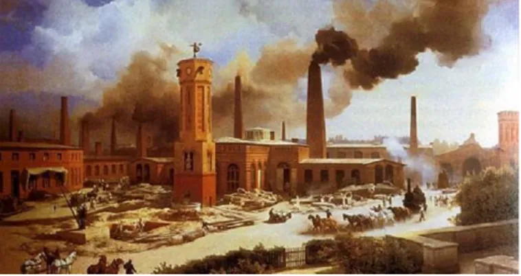
The appearance of the steam engine brings with it the construction and development of a new building-industrial typology, which has acquired by itself a cultural and patrimonial value, very different from the one that was devised: brick factory chimneys.

According to the existing data, the first chimney dates from the first century after Christ. However, the birth of industrial chimneys was in Manchester. In the middle of 18th century, textile factories supposed the building of the first brick chimneys that attracted thousands of people from rural areas. The magnitude of industrial development led to the arrival in the 19th century of huge numbers of immigrants, mainly from Ireland and Italy (Huffpost, 2017).

Fig. 1. Illustration of typical brick chimneys built during the first steps of Industrial Revolution. The primary function, which is derived from the archival sources, refers to hygienist issues, the complaints of neighbours for bad odours and the fumes produced by the lack of height of the chimneys, that is, the conduction of fumes and gases to an enough height that does not harm living beings. The consequent function affects economic terms. The height increasing of the chimney aids the draught of it and, therefore, benefits the combustion, making possible the reduction of the amount of fuel necessary for the generation of steam (Lopez, Martínez and de Mazarredo, 2011).

Moreover, the chimney helps to reduce the concentration of pollutants at ground level, as it allows gases to be diluted along the air column and the concentrations in the ground are very low. Hence, the more chimney height, the better will be dispersion.

1.3. State of the art

Since the first chimney was built, it has been done non-stop improvements in order to enhance their properties and efficiency. Commonly, ameliorations focus in insulating material.

The first idea of insulating was conceived by prehistorical peoples who built temporary dwellings from same materials that they used for clothing. Although, It is not until the end of 19th when rising energy consumption and the relatively high costs of fossil fuels (coal, crude oil) during the worldwide economic crisis (Long Depression, 1873-1896) forced thermal power plants to reduce the heat losses from steam engines, heating equipment, chimneys and also building structures around them. During this period, new building materials emerged (cast-iron, glass structures, concrete, steel, so on) and that supposed the beginning of the first isolating chimneys (Bozsaky, 2011).

Until the middle of the 20th century, most of the chimneys were built of brick, and today they are still true masterpieces of this type of industrial brick architecture. Subsequently, prefabricated concrete blocks were used, which were filled with concrete and with the corresponding steel rods, to assemble the set as it went up in height (Construmatica, 2019).

However, in today’s world the transition towards stainless steel is currently underway. It is the preferred option for renovation because it has a valuable safety features such as a good resistance to soot fires (after inspection, stainless steel chimneys often go back to normal use after an incident) and outstanding shock resistance (the chimney will not tend to break or crack following settlements in the building or even seismic movements). Moreover, stainless steel chimneys are environmentally friendly because their chemical resistance makes them suitable for condensing boilers, which involve the formation of aggressive condensates, their thin walls make them a material-saving option and at the end of the useful life of the building, they are fully recyclable and even have a positive material value (ISSF, 2014).

Apart from insulating materials, the concept of solar chimney power technology has recently been valued. The single solar chimney pilot scheme so far constructed was developed in Spain between 1981 and 1982 at Manzanares and was funded by the German government (Breeze, 2016).

Solar chimney is basically a solar air heater, which is vertically or horizontally embedded as a part of wall or roof. Chimney cavity normally consists of a glazing wall for solar penetration and an absorption wall which allow heat absorption.

The air in the chimney cavity is heated under the penetration of solar radiation through the glazing wall and they rise under the thermal buoyancy to enhance the natural ventilation of buildings. Solar chimney is used to promote natural chimney draught, resulting in the reduction of traditional energy use and the relevant greenhouse gas emission (Shi, 2018).

2. Objectives

The aim of this project is to simulate a conventional chimney in order to know what its dynamics is, and also to check the ANSYS Fluent modelling comparing its results with experimental data.

At the beginning, the learning on how to perform a simulation in ANSYS Fluent, more than a goal is a necessity. And, once learned how to perform simulations with the tool and taking advantage of it, it’s time to define specific objectives:

- To study pressure dynamics throughout a mixture gas of CO2, SO2 and NO2 in

the chimney and make a comparison according to whether the regime is laminar or turbulent.

- To study temperature dynamics throughout a mixture gas of CO2, SO2 and NO2

in the chimney and make a comparison according to whether the regime is laminar or turbulent.

- To study velocity dynamics throughout a mixture gas of CO2, SO2 and NO2 in

the chimney and make a comparison according to whether the regime is laminar or turbulent.

- To incorporate a hypothetical particles flow in order to know how affect to mixture of gases.

3. Material and methods

ANSYS is the software which has been chosen to perform this work. Since was founded in 1970, it has changed the work of academic researchers, allowing them to produce groundbreaking technical research reliably, faster and more cost-effectively than ever.

In classrooms around the world, ANSYS solutions have helped generations of students prepare to tackle real-world engineering challenges. ANSYS student version it’s free, so it grant students the privilege to experience with a wide range of tools in order to deep on simulation and modelling globe.

Moreover, there are a huge amount of manuals and scientific works that let all students understand easier ANSYS software. Still, it’s an intuitive program.

Each day and in every corner of the globe, thousands of engineering faculty, researchers and students leverage the power of ANSYS. Annually, at least 8,000 academic papers and 12,000 dissertations rely on simulations using ANSYS solutions. More than 2,400 teachers have embedded the tools into their engineering curricula, with over 86,000 students enrolled in these classes. Another 10,000 faculty employ the software in academic research (ANSYS, 2014).

Apart from free advantage, another eases which it provides ANSYS to their users are:

- It can model any type of engineering problem. Using ANSYS instead of conducting real experiments, which can be impossible due to the difficulties in creating experimental setup.

- There are a lot of mesh options which allow controlling the mesh and subsequent elements to a high degree. The mesh options combined with the contact options allow for easy modelling of seemingly complex geometry in an easy and structured way.

- Offers the possibility of working in 2D or 3D. Working in 2D or 3D it is useful, but 3D it gives students a better sense of what they are working on.

Although, ANSYS have bad points too, such as:

- ANSYS often can't start the calculation, but it doesn't clarify where the mistake is.

- A powerful and time-consuming computer is required to solve detailed different tasks.

4. Built model

4.1. Geometry design

When a new simulation is started, the first step to do is to set the geometry that is wanted to be simulated. First of all, it’s important to check in the properties if the geometry can be ruled in 2D symmetry, as it would be easier and faster to obtain the results afterwards.

So, to do it, ANSYS offer a wide range of analysis systems tools, but it has been used Fluid Flow (Fluent) because it is which fits better. Once tool has chosen, it is when the chimney design can be carry on. There are two internal options to design the chimney, Design Modeler or Space Claim. It has picked out the first one as there are more manuals and information about it than the other one. Although, another choice is to import, in the workbench, geometry already created from other software such as Solid Edge, AutoCad, so on, but it is not this case.

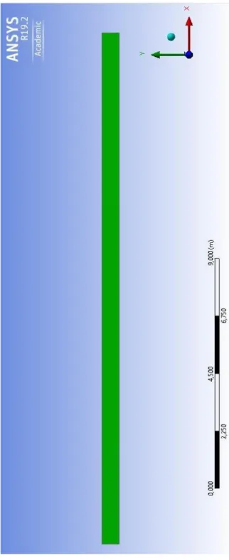
The system in study has a high symmetry, and it is why allows to perform the project in 2D. The dimensions of the chimney have been fixed according to the Spanish law (RD 100/2011) stating that the minimum height for industrial chimneys must be at least 10 meters high above ground level:

- Height: 20 m - Diameter: 0.7 m

The design of the chimney is shown in the figure 1 and the steps realised to get it has been the next ones:

1. Defining geometry as 2D.

2. Creating a new sketch in XYPlane.

3. Setting a grid with a major space setting of 20 m.

4. Starting the design using sketching toolboxes. The first one it is draw the chimney employing rectangle tool.

5. Dimensioning of the chimney utilizing general tool, and then applying the correct values of height and diameter.

6. Defining geometry as a surface through Surface from Sketches option.

Once geometry has been already created, the next step is starting meshing, the last step before commencing setup.

4.2. Meshing generation

After doing the geometry, it is proceeding meshing operation. The mesh influences the accuracy, convergence and speed of the solution. It is a fundamental part of the analysis because of doing a correct mesh, guarantee nearly real results.

The basic idea of ANSYS is to make calculations at only limited (finite) number of points and then interpolate the results for the entire domain (surface or volume). Any continuous object has infinite degrees of freedom and it’s just not possible to solve the problem in this format. Therefore, using meshing it is reducing the degrees of freedom from infinite to finite (nodes).

The solution it’s never completely exact, but if the distance of the finite point is reduced, the approximation will be more accurate. Nonetheless, smaller mesh entails raise up the number of the nodes. Increasing the number of the nodes involve a major computational time to perform the simulation. Furthermore, in the ANSYS student license the number of nodes that can be used is limited, in this case there are 500,000.

So as to reduce the errors, ANSYS allows the creation of inflation zones which let increasing the number of the nodes, especially in the points where is highly probable that the values could suffer strong variations (i.e. inlet and outlet of the chimney).

The tools used to get a refined mesh have been the following ones:

- Face meshing: Controls enable to generate a free or mapped mesh on selected faces. It is the initial step of the mesh refinement, when it is indicated in which face will be have mesh.

- Refinement: Controls specify the maximum number of meshing refinements that are applied to the initial mesh. Refinement controls are valid for faces, edges, and vertices.

- Sizing: The sizing control sets the number of divisions along an edge. In this work, two edges sizing have been assigned. One related onto inlet and outlet flow of the chimney, where the number of divisions allocated is 20. The second one is related to walls of the chimney, and the number of divisions allotted is 100.

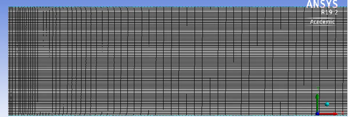
Fig. 3. First sight of the mesh. Clearly, the refinement it’s plausible to allow make accurate calculations.

Fig. 4. Zoom of the mesh. The inlet and outlet are high-meshed as they are strategic points because are the base of calculations, therefore, it's necessary for the program to make a good

convergence.

4.3. Simulation setup

4.3.1. Validation model

The next step in ANSYS simulation is the setup. Fluent also have different additional models that can be activated depending on the system. In this case, two more additional models must be activated to perform the simulation as accurately as possible (energy and turbulent k-ε models).

At first, it has been validated the model to apply different conditions afterwards. To prove the model, it has been considered only air and the next boundary conditions:

- 2D space is an axisymmetric, so the axis of symmetry must coincide with the global y-axis. The geometry must lie on the positive x-axis of the x-y plane. - Gravitational acceleration is -9.8 m/s2_.

- It has been chosen velocity (inlet), pressure (outlet) and temperature magnitudes.

Velocity-inlet is 2.13 m/s (turbulent regime) and pressure-outlet is 0 Pa (Zhou et.al, 2007). Flue gas inlet temperatures ranging among 100 – 300 oC (Chu, 2019) and it has been selected 127 oC (400 K).

- Moreover, one of the walls it has been named as an axis and the other one as a wall.

Once conditions have been prefixed, it has been performed many iterations have been performed considering velocity, until the model has converged. Furthermore, the matter balance decreased too.

The following figures demonstrate that the model it is meaningful, as in real conditions it occurs similar. Pressure outlet is lower than pressure inlet, and velocity and temperatures are higher in the middle of the chimney than near to the wall

Outlet pressure has to be lower than inlet pressure in order to allow the expelling of the combustion gases. The difference between both pressures it is known as a chimney draught.

Velocity is higher in the middle of the chimney than in the walls due to the friction force, that it reduces the speed when it approaches to the walls.

The temperature drops slightly because it is none an adiabatic model, so the loss of heat is unavoidable.

Fig. 6. Contour of velocity range between wall zones and the middle of the chimney in turbulent regime.

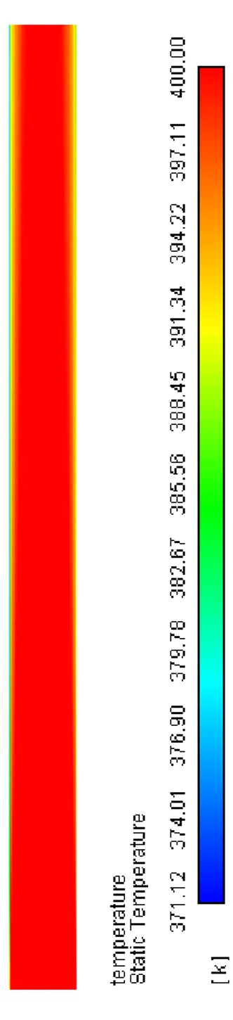
Fig. 7. Distribution of temperatures along the chimney from inlet until to outlet in turbulent regime.

4.3.2. Models applicated

Once the model has been validated, it’s time to choose the correct models, the boundary conditions, the mesh interfaces, etc. It is essential to establish the correct conditions in order to obtain a reliable solution.

In the model definition, one must consider the mathematical model that will be carried out to analyse the process. In this work, two parallel studies are put through. Both fluent cases include energy model and discrete phase model. The difference remains on the viscous model. One study has been made with laminar model and the other one with turbulent k-ε model.

Energy model allows to set parameters related to energy or heat transfer in the model. The main idea is to see how variate temperature along the chimney, as the model is non-adiabatic and determine the heat loss through the walls.

Discrete Phase model allows setting parameters related to the calculation of a discrete phase of particles using injection option. The initial conditions that it has been provided for the discrete phase calculations in ANSYS Fluent are diameter (10 µm), temperature (560 K) and flow rate (1·10-20 kg/s) according to more commons values (Gogoi, Choudhury and Ahmed, 2010).

Viscous models must be activated because there is a natural fluid flow through the system. Laminar flow occurs when the fluid flows in infinitesimal parallel layers with no disruption between them. In laminar flows, fluid layers slide in parallel, with no eddies, swirls or currents normal to the flow itself. Turbulent flow refers to irregular flows in which eddies, swirls and flow instabilities occur (Simscale, 2019). In the table below, it summarises the main parameters in both regimes.

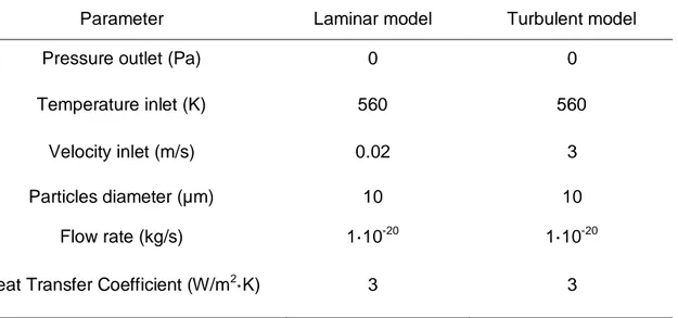
Table 1. Summary of parameters in both models purposed.

Parameter Laminar model Turbulent model

Pressure outlet (Pa) 0 0

Temperature inlet (K) 560 560

Velocity inlet (m/s) 0.02 3

Particles diameter (µm) 10 10

Flow rate (kg/s) 1·10-20 1·10-20

Heat Transfer Coefficient (W/m2·K) 3 3

ANSYS fluent solves each model using a wide range of the equations. The following ones are which have been used on this frame.



Where p is the static pressure, is the stress tensor, ρ



Where keff is the effective conductivity (k + kt, where kt is the turbulent thermal

conductivity, defined according to the turbulence model being used), and j is the

diffusion flux of species j. Sh includes the heat of chemical reaction, and any other



Where Fx is an additional acceleration (force/unit particle mass) term, FD (u - up) is the

drag force per unit particle mass, u is the fluid phase velocity, up is the particle

velocity, µ is the molecular viscosity of the fluid, ρ is the fluid density, ρp is the density

of the particle, and dp is the particle diameter.

Apart from these equations, there are some equations related to laminar and turbulent equations but are out of the range of this study. The general equation for both regimes is (Cordoba, 2011):

Where ρ is the density of the mixture, µ the viscosity, D the diameter and fv an external

force.

5. Results and discussion

As described before, the most important variables to analyse in a conventional chimney are pressure, temperature and velocity in each point of the system. Therefore, their profiles, contours and distributions will be discussed comparing laminar and turbulent regimes.

Furthermore, are going to be shown other results such as the energy balance and the graphics of inlet length and flow stabilization in order to understand the developing velocity profile of a fluid entering a tube, which distinguish onto two phases: hydrodynamic entrance region and fully developed region.

Moreover, there is a need to say that the graphics will be done with excel and contours have been exported from ANSYS.

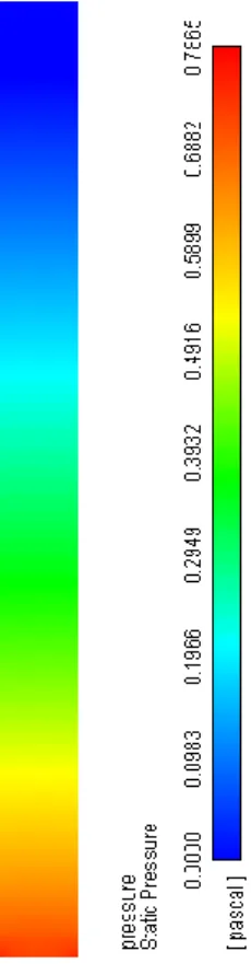
5.1. Pressure contours

The pressure contours of mixture and mixture with particles are going to be shown below comparing laminar and turbulent regime.

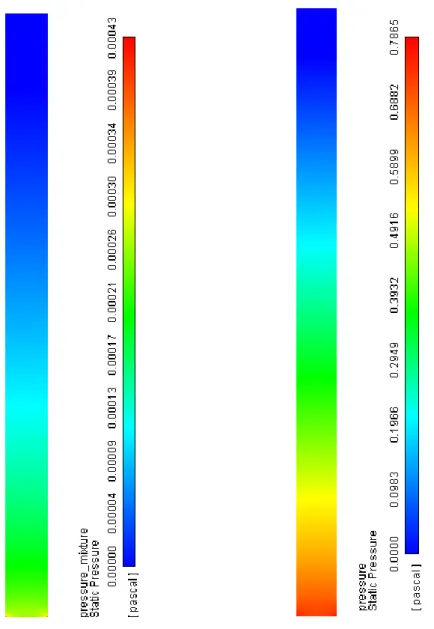
Fig. 8. Gas mixture pressure contours for both regimes, laminar (left) and turbulent (right). Axis symmetric applied.

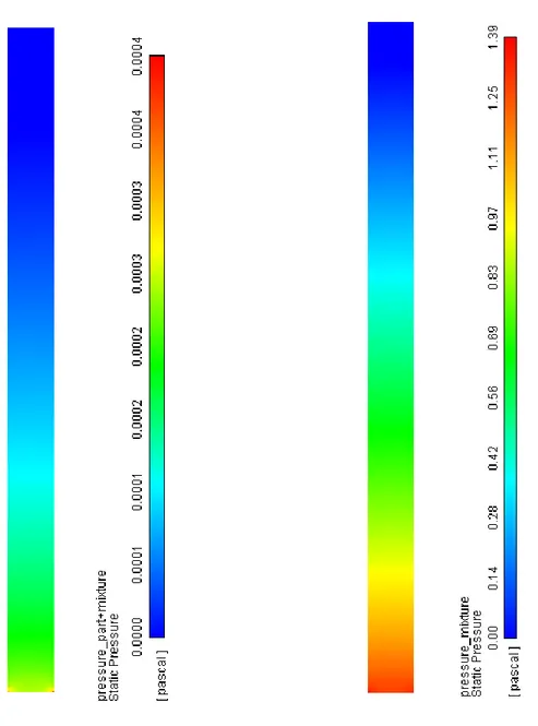
Fig. 9. Pressure contours of gas mixture with particles for both regimes, laminar (left) and turbulent (right). Axis symmetric applied.

In the figures 8 and 9 where the pressure contours for both models are shown, it’s important to consider the outlet pressure. It has been calculated as a Gauge pressure which is the difference between absolute pressure and atmospheric pressure.

Figure 8 shows that the range of pressures for the turbulent regime is higher because it is a more heterogeneous flow, there will be more contact with the walls of the chimney. This fact entails a greater loss of pressure along the path of the mixture through the chimney, whereby the inlet pressure must be higher when there is a turbulent regime.

In Figure 9, it is observed that the laminar regime undergoes slight variations when a stream of particles is added. While the turbulent regime case, outstands that inlet pressure is higher, in order to get over friction force caused by particles.

5.2. Temperature contours and graphics

The temperature contours of gases mixture and mixture with particles are going to be shown below comparing laminar and turbulent regime. Also, it has been represented the temperature of each gas in 3 different points (inlet, middle and outlet) in both regimes.

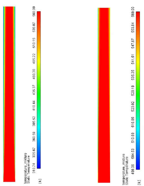
Fig. 10. Gas mixture temperature contours for both regimes, laminar (left) and turbulent (right). Axis symmetric applied.

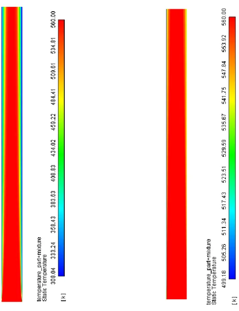
Fig. 11. Temperature contours of gas mixture with particles for both regimes, laminar (left) and turbulent (right). Axis symmetric applied.

CO2 SO2 NO2

CO2 SO2 NO2

Fig. 12. Distribution of temperatures in 3 points (inlet, middle and outlet) in laminar regime for each gas which compounds the mixture.

Fig. 13. Distribution of temperatures in 3 points (inlet, middle and outlet) in turbulent regime for each gas which compounds the mixture.

NO2 SO2 CO2 100 0 Inlet Middle Outlet 600 500 400 300 200 NO2 SO2 CO2 100 0 Inlet Middle Outlet 600 500 400 300 200 Te m p e ra tu re ( o C) Te m p e ra tu re ( oC)

In figures 10 and 11 where the temperature distribution is shown, it is important to consider the chimney inlet. The inlet temperature is 560 K for both models according to Chu (2019), with this temperature at the beginning of the simulation; the contours complete the energy equations showing the temperature distributions. The heat flow goes to the pipe wall by convection heat transfer through the fluid which leads to the decrease of temperature.

In both models, regardless of the regime, it is observed that the temperature is higher near to the inlet of the chimney. It occurs because the heat is transmitted horizontally from the higher temperature region to the lower temperature region. The inlet is the starting point, so there is where will be a greater transfer of heat. As the flow is going up the chimney, it is cooling down, therefore, the heat exchange will be less and the wall will be cooler at the outlet than at the inlet (Fernandez, 2019).

Comparing the laminar regime with the turbulent one, it is observed that the temperature decreases much more near to the walls when the flow is laminar as there are conditions in which the flow does not separate from the wall of the tube. This causes an inefficient heat transfer because at high temperatures the viscosity increases in the adjacencies of the wall, and this goes up the resistance to heat flow. Hence, the part of the fluid that is stuck to the wall exchanges more heat than the part located in the middle according to Navrose and Mittal, (2019).

Moreover, when the fluid contains particular matter, increases even more the resistance of the flow, so the differences among temperatures near to the wall and in the middle of the chimney rise up.

In addition, a universally useful technique has emerged. Consisting in deforming the tube with a continuous groove or indentation in spiral along the same, or intermittent point indentations. For values of the Reynolds number above 10,000, this type of deformation also significantly increases the amount of turbulence and, therefore, the heat exchange ratio, which if properly balanced together with other factors, can help reduce the total area of exchange required and also the economic costs.

Furthermore, in figures 12 and 13 it is shown the temperature variation, for both regimes, of each gas which compounds the mixture. As described before, when exists a laminar regime, the difference of temperatures between the 3 selected points it is more notorious.

Besides that, the temperature difference between the gases can be due to the density and heat capacity (Cp). The denser is the gas, the lower temperature changes occur.

In addition, the heat capacity is major, the higher temperatures occur. According to datafluent base of ANSYS, it has been observed that SO2 is the denser gas (CO2 and

NO2 has the same density) and which has a lower value of heat capacity. In the table

below, it has shown the ANSYS database:

Table 2. Datafluent base of ANSYS for each gas considered in the present study.

Parameter CO2 SO2 NO2

Density (kg/m3) 1.79 2.77 1.79

5.3. Velocity contours, vectors and graphics

The velocity contours of mixture and mixture with particles are going to be shown below comparing laminar and turbulent regime. Also, it has been represented the velocity of each gas in 3 different points (inlet, middle and outlet) in both regimes, and vectors diagrams near to the walls and in the middle of the flow towards understand the behaviour of laminar and turbulent regimes.

Fig. 14. Gas mixture velocity contours for both regimes, laminar (left) and turbulent (right). Axis symmetric applied.

Fig. 11. Velocity contours of gas mixture with particles for both regimes, laminar (left) and turbulent (right). Axis symmetric applied.

Fig. 12. Vectors representing the dynamics of the fluid in laminar regime at the inlet (left), in the middle and at the outlet of the chimney (right).

Fig. 13. Vectors representing the dynamics of the fluid in turbulent regime at the inlet (left), in the middle and at the outlet of the chimney (right).

CO2 SO2 NO2

CO2 SO2 NO2

Fig. 14. Distribution of velocities in 3 points (inlet, middle and outlet) in laminar regime for each gas which compounds the mixture.

Fig. 15. Distribution of velocities in 3 points (inlet, middle and outlet) in turbulent regime for each gas which compounds the mixture.

NO2 SO2 CO2 0,005 0,000 Inlet Middle Outlet 0,030 0,025 0,020 0,015 0,010 NO2 SO2 CO2 0,50 0,00 Inlet Middle Outlet 3,50 3,00 2,50 2,00 1,50 1,00 V e lo ci ty (m /s) V e lo cit y (m /s)

The velocity is a complex variable which leads to understand more the fluid behavior in the chimney. In order to appreciate better the differences between both regimes, it has been represented the velocity vectors (figures 12 and 13). It is shown as in turbulent regime the flux is more heterogeneous than in laminar flux (Heat exchangers, 2017).

Regardless of the regime, the velocity only decreases near to the walls due to the friction that the fluid suffers. The differences are more plausible in laminar regime because of a wide part of the flow stay in contact during the ascent, according to the characteristics of this kind of regime as It describe in the last section.

At first sight, it seems that particles have not an effect in the velocity, but it's not like that. Although it's difficult to distinguish the difference among both models (with or without particles), it is clear that in a real situation particles are an issue. Unlike gases, particles do not rise inherently. Being solid matter, tend to descend due to the gravity force. Moreover, whether flow presents particles in the fluid leads to a greater loss of charge (Aula virtual, 2019).

Particles imply an increase of operability costs. Likely, when a flow is loaded with solid matter, it is unthinkable that the natural draft of the chimney will be enough in order to get gases expelled. Then, it will be a request use fans that increase the velocity along the chimney, in order to completely evacuate the flow resulting from combustion.

Another option is implement some equipment before the chimney, which allows reducing the particles load in the flow. Depending on the particle size and the outlet temperature of combustion chamber, there are a few options. The first one is a cyclone, which is the cheaper machine, but it has a restriction size (no separation under 10 µm; in that case is in the limit). Still, the following options are electrostatic precipitator and baghouse filter. The first one may works at high temperature but it is not adaptable to operating conditions; the second one is more efficient, but the trouble is that only works out until 150 ºC, so it is necessary to install a heat exchanger. There is a wide range of options, but care must be taken when deciding which the best option is.

In figures 14 and 15, it is shown the velocity distribution of each gas of the mixture. The whole velocities have been calculated in the middle of the chimney. It is demonstrated that there is hardly difference among gases in both regimes. In contrast of the particles, gases have natural ascending behavior. In that case, three gases have a similar density, so the ascending dynamic is nearly exactly the same.

5.4. Energy balance, inlet length and flow stabilization

In the following section, it has been shown the graphics of hydrodynamic length in order to know when the velocity profile is uniform. Furthermore, it has been realized the energy balance to equilibrate the system.

Velocity has been calculated through surface integrals option. Some points have been defined along the chimney and then from Area-Weighted Average choice, it has been determine the velocity in each point.

The surface velocity integrals of each point are shown in table 2 for both models, laminar and turbulent.

Table 3. Velocity surface integrals in each point. In this case, each point represents

one height in meters from inlet (0 m) to outlet (20 m).

Point Laminar regime Point Turbulent regime

Inlet 0.0200 Inlet 3.00 1 0.0210 1 3.02 2 0.0220 2 3.05 3 0.0232 3 3.07 4 0.0239 5 3.10 6 0.0249 7 3.14 8 0.0260 9 3.20 10 0.0264 10 3.25 11 0.0267 12 3.28 12 0.0269 14 3.30 13 0.0270 16 3.30 15 0.0270 17 3.30 17 0.0270 18 3.30 19 0.0270 19 3.30 Outlet 0.0270 Outlet 3.30

The calculation of hydrodynamic length varies depending on the regime. The length required for the velocity profile in laminar flow to be invariant in contrast to the axial position, is the hydrodynamic input length LH that can be approximated by the Langhaar equation (Fernandez, 2019):

Lhy,lam ≈ 0.05 𝑅𝑒 𝐷

Where R is the Reynolds number and D is the diameter.

In turbulent regime, the equation is simpler than in laminar regime. It has shown below (Aliev,1995):

Lhy,turb ≈ 10 𝐷

Fig. 16. Hydrodynamic length graphic using velocity as a variable for laminar regime. Blue line means the velocity in each point and red line means the empiric calculated length.

Fig. 16. Hydrodynamic length graphic using velocity as a variable for turbulent regime. Blue line means the velocity in each point and red line means the empiric calculated length.

Height (m) 25 20 15 10 5 Theoric lenght (m) 0 Velocity (m/s) 0,029 0,028 0,027 0,026 0,025 0,024 0,023 0,022 0,021 0,020 0,019 3,40 3,35 3,30 3,25 3,20 3,15 3,10 3,05 3,00 2,95 2,90 Velocity (m/s) Theoric lenght (m) 0 5 10 15 20 25 Height (m) V e lo ci ty (m /s) V e lo ci ty (m /s)

Comparing the hydrodynamic length calculated empirically with the experimental one, it is observed that they do not coincide (Table 3).

Table 4. Comparison of hydrodynamic length among calculated throughout the

equations and simulated with ANSYS.

Laminar regime Turbulent regime

Theorical length (m) 4 7

Simulated length (m) 12 10

Probably, the turbulent regime being more heterogeneous makes it easier to calculate the hydrodynamic length and that is why it is less far from the one computed by the software.

And to sum up the study, it has been equilibrated the system, calculating the energetic balance from the typical equation:

Q = (w · Cp · (Ti – T*)) – (w · Cp · (To – T*)

Where the w is the mass flow, Cp is the specific heat, Ti is the inlet temperature

(Ti = 560 K), To is the outlet temperature (To = 554 K) and T* is the reference

temperature (T* = 273 K).

The table below (Table 4) summarises the energetic balance in each regime:

Table 5. Energetic balance for both kinds of regimes.

Laminar regime Turbulent regime

W (kg/s) 0.01 1.42

Q (J/s) 69.53 10,428.82

Energetic balance shows that in turbulent regime the heat loss rate is higher than in laminar one. According to the characteristics of each regime is logical, so in laminar system the low heat transfer carries to a less heat loss.

6. Conclusions

- After studying the internal dynamics of a conventional industrial chimney it can be stated that there are differences between laminar and turbulent regimes in each of variables which have been studied. The flow behavior, in both regimes, is similar in the middle of the chimney and close to the walls, but the differences are clearer in laminar regime as the flow is more homogeneous. The clearest differences, remains in hydrodynamic length, where according to ANSYS, velocity profile will be uniform in turbulent regime (10 m) before than the laminar (12 m). Moreover, another difference is stated in energetic balance, which shows that the heat loss is higher in turbulent regime (10,428.82 J/s; in laminar regime is 69.53 J/s).

- After studying the internal dynamics of a conventional industrial chimney in ANSYS® Fluent, it can be observed that particles modify slightly both models. Changes are not outstanding in contrast with mixture gases model, as the particles injection is low so it is just a simple simulation for further works that will include it more widely. The clearest differences are in turbulent pressure contours (inlet pressure without particles is 0.7865 Pa, and with particles is 1.39 Pa) and in laminar temperature contours (lower temperature without particles is 311 K and with particles is 308 K)

- Considering that the main goal of the study is to compare the results of mixture gases between laminar and turbulent regime, both models are equally valid, but the turbulent model is more representative.

- Validated the results for both models, it is possible to say that the obtained results of pressure, temperature and velocity are expected to match with a real situation.

- The project can be extended for further works, for example, adding a model with an atmosphere that allows simulating the dispersion. Furthermore, it can change the flow composition.

7. References

About ANSYS, 2019. ANSYS [online]. [viewed 26th March 2019]. Available in: https://www.ansys.com/about-ansys

ALIEV, Ruslan. 2015. CFD Investigation of Heat Exchangers with Circular and Elliptic

Cross-Sectional Channels. Doctoral thesis. Cleveland State University. Department of

Mechanical Engineering.

ANSYS, 2014. Spotlight on academics. ANSYS advantage, 8, issue 1. [online]. [viewed

25th March 2019]. Available in: https://www.ansys.com/-

/media/ansys/corporate/resourcelibrary/article/ansys-advantage-academic-aa-v8-i1.pdf

Aula virtual, 2019. Intercambio de calor por conducción. [online]. [viewed 13th June

2019]. Available in: http://www.aulavirtual-

exactas.dyndns.org/claroline/backends/download.php?url=L0NPTlZFQ0NJT04vRWN1 YWNpb25lc19lbXDtcmljYXNfMi5wZGY%3D&cidReset=true&cidReq=FUTRCAMA

Batchelor, G.K, 1967. An Introduction to Fluid Dynamics. Cambridge University Press, Cambridge, England.

Bozsaky, D., 2011. The historical development of thermal insulation materials.

Periodica polytechnica, 41, 49-56.

Bradshaw, P., Ferriss, D.H. and Atwell, N.P., 2006. Calculation of boundary-layer development using the turbulent energy equation. Journal of Fluid Mechanics, 28, 593- 616.

Breeze, P., 2016. Solar power generation. Academic Press Books, 7, 47-50.

Construmatica: Portal de arquitectura e ingeniería [viewed 30th May 2019]. Available in:

https://www.construmatica.com/construpedia/Chimeneas_Industriales#Bibliograf.C3.ADa Cordoba, D., 2011. Las ecuaciones de Navier-Stokes. Jornadas sobre los problemes

del milenio. [online.] [viewed 9th June 2019]. Available in:

http://garf.ub.es/Milenio/img/Navier-Stokes.pdf

Fernández, P, 2019. Transmisión de calor por convección. Flujo en conductos. [online].

[viewed 12th June 2019]. Available in:

http://webcache.googleusercontent.com/search?q=cache:GIWueChfYigJ:manager.red sauce.net/AppController/commands_RSM/api/api_getFile.php%3FitemID%3D96%26pr

opertyID%3D20%26RStoken%3D59e8ac1045d03e2ff6564c0638315f38+&cd=1&hl=ca &ct=clnk&gl=es

Gogoi, A., Choudhury, A. and Ahmed, G., 2010. Mie scattering computation of spherical particles with very large size parameters using an improved program with variable speed and accuracy. Journal of Modern Optics, 57, 2192 – 2202.

Heat exchangers, 2016. Comparación entre flujo laminar y turbulento. [online]. [viewed

11th June 2019]. Available in: https://www.hrs-

heatexchangers.com/es/recursos/comparacion-entre-flujo-laminar-y-turbulento/

Huffpost, 2017. Manchester, viaje a las raíces de la Revolución Industrial. [viewed 30th May 2019]. Available in: https://www.huffingtonpost.es/ruben-alonso/manchester-viaje-a- las-raices-de-la-revolucion-industrial_a_23262434/

ISSF: International Stainless Steel Forum, 2014 [viewed 28th May 2019]. Available in:

http://www.worldstainless.org/Files/issf/non-image-files/PDF/Euro_Inox/Chimneys_EN.pdf López, P., Martínez, A. and de Mazarredo, L., 2011. Chimeneas industriales de ladrillo helicoidales. Conference: Actas del Séptimo Congreso Nacional de Historia de la

Construcción. At: Santiago de Compostela.

Metropolis, N. and Ulam, S., 2012. The Monte Carlo Method. The Journal of the

American Statistical Association, 44, 335-341.

NANCE, Richard and OVERSTREET, Michael, 2017. History of computer simulation

software: An initial perspective. Las Vegas: IEEE. ISSN: 1558-4305.

Navrose and Mittal, S., 2019. Intermittency in free vibration of a cylinder beyond the laminar regime. Journal of Fluid Mechanics, 870, R2.

NYGAARD, Kristen and DAHL, Ole-Johan, 1981. The Development of the SIMULA

Languages. University of Oslo. ISBN: 0-12-745040-8.

Real Decreto 100/2011, de 28 de enero, por el que se actualiza el catálogo de actividades potencialmente contaminadoras de la atmósfera y se establecen las disposiciones básicas para su aplicación.

Schuster, E.F., 1974. Buffon's Needle Experiment. The American Mathematical

Monthly, 81, 26-29.

Shi, L., 2018. Theoretical models for wall solar chimney under cooling and heating modes considering room configuration. Energy, 165, 925-938.

Simscale, 2019. [online]. [viewed 9th June 2019]. Available in: https://www.simscale.com/

Talbot, L., 1980. Thermophoresis of particles in a heated boundary layer. Journal of

Fluid Mechanics, 101, 737-758.

Timelines, 2019. Preceden [online] [data query: 26 March 2019]. Available in: https://www.preceden.com/timelines/297649-historia-simulacion

Toja-Silva, F., Pregel-Hoderlein, C. and Chen, J., 2018. On the urban geometry generalization for CFD simulation of gas dispersion from chimneys: Comparison with Gaussian plume model. Journal of Wind Engineering & Industrial Aerodynamics, 177, 1-18.

Ulam, S., 1979. John von Newman 1903 – 1957. American Mathematical Society, 64, 1-49.