Applying Generalized Continuous Time Bayesian Networks to a reliability case study

(1)

ScienceDirect

IFAC-PapersOnLine 48-21 (2015) 676–681

Available online at www.sciencedirect.com

10.1016/j.ifacol.2015.09.605

Daniele Codetta-Raiteri et al. / IFAC-PapersOnLine 48-21 (2015) 676–681

Applying Generalized Continuous Time

Bayesian Networks to a reliability case

study

Daniele Codetta-Raiteri∗

∗_{DiSIT, Computer Science Institute, University of Piemonte} Orientale, Alessandria, Italy (e-mail: dcr@di.unipmn.it).

Abstract: We discuss the main features of Generalized Continuous Time Bayesian Networks (GCTBN) as a reliability formalism: we resort to a specific case study taken from the literature, and we discuss modeling choices, analysis results and advantages with respect to other formalisms. From the modeling point of view, GTCBN can represent dependencies involving system components, together with the possibility of a continuous time evaluation of the model. From the analysis point of view, any task ascribable to a posterior probability computation can be implemented, such as the computation of system unreliability, importance (sensitivity) indices, system state prediction and diagnosis.

Keywords: generalized continuous time Bayesian networks, reliability analysis, diagnosis, sensitivity analysis, probabilistic models.

1. INTRODUCTION

In reliability analysis, Bayesian Networks (BN) (Langseth and Portinale (2007)) are an interesting trade-off between combinatorial models (e.g. Fault Trees, Reliability Block Diagrams, etc.) and state space-based models (e.g. Markov Chains, Petri Nets, etc.) (Sahner et al. (1996)). Standard BN are however static models representing a snapshot of the system at a given time point. When time is taken into account, the main choice concerns whether to consider it as a discrete or a continuous dimension. In the first case, Dynamic Bayesian Networks (DBN) (Murphy (2002)) have become a natural choice; in the second case, Contin-uous Time Bayesian Networks (CTBN) (Nodelman et al. (2002)) have started to be investigated. In Codetta and Portinale (2013) Generalized Continuous Time Bayesian Networks (GCTBN) are proposed by allowing the pres-ence of nodes which have no explicit temporal evolution; their values are “immediately” determined, depending on the values of other nodes. This allows us to model processes having both a continuous-time temporal dimension and a static dimension (logical/probabilistic aspects).

In this paper we show how GCTBN (Sec. 2) can be suitably used to compute dependability measures like system unreliability, importance indices, and diagnostic measures. We show that GCTBN can be adopted to model dependencies among components, like those introduced in Dynamic Fault Trees (DFT) (Dugan et al. (1992)). Also in this case, it is very important to distinguish, at the modeling level, between delayed and immediate entities. Furthermore, other kinds of dependencies can be captured through GCTBN. We resort to a specific case study and we discuss: modeling choices (Sec. 3), analysis results (Sec. 4), and advantages with respect to DBN (Sec. 5).

2. FORMAL DEFINITIONS 2.1 Dynamic Fault Trees

Fault Trees (FT) (Sahner et al. (1996)) represent how the failure propagates from the components (basic events) to the system (top event); Boolean gates (AND, OR, k out of n (k:n), etc.) are used to this end. DFT augment FT with dynamic gates; in the DFT model of the case study (Sec. 3.1) we use the following ones.

Functional Dependency gate (FDEP): given a trigger event T and a set of dependent events D1, . . . , Dn, when T occurs, D1, . . . , Dn are immediately forced to occur. Cold Spare gate (CSP): given a set of spares S1, . . . , Sn able to replace a main component M when it fails, the output event occurs if M has failed and there are no spares available to replace it. A spare can be in three states (dormant, working, failed) and its failure rate changes depending on its current state: λ if working, 0 if dormant. 2.2 Dynamic Bayesian Networks

Given a set of time-dependent state variables X1, . . . , Xn, and given a BN N defined on such variables, a DBN is essentially a replication of N over two time slices t − ∆ and t (being ∆ the so called time discretization step), with the addition of a set of arcs representing the transition model. Let Xt

i denote the copy of variable Xi at time slice t, the transition model is defined through a distribution P [Xt

i|Xit−∆, Yt−∆, Yt] where Yt−∆is any set of variables at slice t − ∆ different from Xi (possibly the empty set), and Yt _{is any set of variables at slice t different from X}

i (possibly the empty set).

An edge connecting a variable Xt−∆

i in the slice t − ∆ to the same variable Xt

i in the slice t, is called temporal

9th IFAC Symposium on Fault Detection, Supervision and Safety of Technical Processes

September 2-4, 2015. Arts et Métiers ParisTech, Paris, France

Applying Generalized Continuous Time

Bayesian Networks to a reliability case

study

1. INTRODUCTION

Applying Generalized Continuous Time

Bayesian Networks to a reliability case

study

1. INTRODUCTION

Applying Generalized Continuous Time

Bayesian Networks to a reliability case

study

1. INTRODUCTION

i|X t−∆

i , Yt−∆, Yt] where Yt−∆is any set of variables at slice t − ∆ different from Xi (possibly the empty set), and Yt _{is any set of variables at slice t different from X}

Applying Generalized Continuous Time

Bayesian Networks to a reliability case

study

1. INTRODUCTION

i|X t−∆

i , Yt−∆, Yt] where Yt−∆is any set of variables at slice t − ∆ different from Xi (possibly the empty set), and Yt _{is any set of variables at slice t different from X}

(2)

Applying Generalized Continuous Time

Bayesian Networks to a reliability case

study

1. INTRODUCTION

i|Xit−∆, Yt−∆, Yt] where Yt−∆ is any set of variables at slice t − ∆ different from Xi (possibly the empty set), and Yt _{is any set of variables at slice t different from X}

Applying Generalized Continuous Time

Bayesian Networks to a reliability case

study

1. INTRODUCTION

Applying Generalized Continuous Time

Bayesian Networks to a reliability case

study

1. INTRODUCTION

Applying Generalized Continuous Time

Bayesian Networks to a reliability case

study

1. INTRODUCTION

i|X t−∆

i , Yt−∆, Yt] where Yt−∆ is any set of variables at slice t − ∆ different from Xi (possibly the empty set), and Yt _{is any set of variables at slice t different from X}

Applying Generalized Continuous Time

Bayesian Networks to a reliability case

study

1. INTRODUCTION

i|X t−∆

i , Yt−∆, Yt] where Yt−∆ is any set of variables at slice t − ∆ different from Xi (possibly the empty set), and Yt _{is any set of variables at slice t different from X}

arc. The dependency of a certain node on its parent nodes (possibly including its historical copy) is quantified in its Conditional Probability Table (CPT).

2.3 Generalized Continuous Time Bayesian Networks Given a set of discrete variables V = {X1, . . . , Xn} partitioned into the sets D (delayed variables) and I (immediate variables), a GCTBN is a pair P0

V, G where P0

V is an initial probability distribution over D;

G is a directed graph whose nodes are X1, . . . , Xn (with P a(Xi) denoting the parents of Xi in G) such that

• there is no directed cycle in G composed only by nodes in the set I;

• for each node X ∈ I a CPT P [X|P a(X)] is defined (as in standard BN and DBN);

• for each node X ∈ D a Conditional Intensity Matrix (CIM) QX|P a(X) is defined (as in CTBN). The CIM of a variable X provides the transition rates for each possible couple of values of X.

Delayed nodes represent variables with a continuous time evolution; they are ruled by exponential transition rates conditioned by the values of parent variables (that may be either delayed or immediate). Each delayed node has a CIM. Immediate nodes instead, are introduced in order to capture variables whose evolution is not ruled by transition rates, but is conditionally determined, at a given time point, by other variables in the model. Therefore immediate nodes are treated as usual chance nodes in a BN: each immediate node has a standard CPT.

Stochastic process. The evolution of a system modeled through a GCTBN occurs as follows: the initial state is given by the assignment of the initial values of the variables, according to P0

V. Given the current system state (represented by the joint assignment of the model variables, both delayed and immediate), a value transition of a delayed variable Dk will occur, after an exponentially distributed delay, by producing a new state called a “vanishing state”. Given the new vanishing state, a new assignment is determined to any immediate variable Ij such that Dk belongs to the set of the “Closest” Delayed Ancestors (CDA) of Ij(composed by any delayed variable Di such that a path from Di to Ij exists and contains no intermediate delayed nodes). The assignment to Ij is consistent with the CPT of Ij. The resulting state, called a “tangible state”, is the new actual state of the system, from which the evolution can proceed with a new transition of value by a delayed variable.

2.4 Inference tasks

The analysis (inference) of a DBN or GCTBN model computes the probability at a given time point, of a set of variables of interest, conditioned on the evidence which is a set of time stamped observations. Two inference tasks can be performed.

Prediction consists in computing the posterior probability at time t of a set of queried variables Q ⊆ (D ∪ I), given a stream of observations et1, . . . , etk from time t1 to time

tk with t1< . . . < tk ≤ t. Every evidence etj consists of a

(possibly different) set of instantiated variables. A special case called Monitoring occurs when the last evidence time point and the query time are the same.

Smoothing consists in computing the probability at time t of a set of queried variables Q ⊆ (D ∪ I), given a stream of observations et1, . . . , etk from time t1 to time tk with

t < t1< . . . < tk.

3. A DEMONSTRATIVE CASE STUDY

We take into consideration the case study called Hypo-thetical Sprinkler System (HSS) (Bobbio et al. (2008)), composed of three sensors, two pumps, and one digital con-troller (Fig. 1). The sensors send signals to the concon-troller, and when temperature readings at two of the sensors are above threshold, the controller activates one of the pumps. 3.1 DFT model

The failure mode of the system can be modeled in a preliminary way using the DFT in Fig. 2. Each compo-nent is represented by a basic event characterized by the failure rate (Tab. 1) according to the negative exponential distribution ruling the random time to failure. A pump cannot work if its support stream (valve and filter) is down; this is captured by the FDEP gates. The pumps are two: the backup pump (“cold” spare (Sec. 2.1)) is activated only if the primary pump fails; the CSP gate is used to model this relationship, and its output event is PumpFault. The 2:3 gate over the sensors has SensorFault as output event. The system failure (top event) occurs when the sensor subsystem fails (event SensorFault), or the digital controller fails (basic event DigCon), or the pump subsystem fails (event PumpFault).

The present paper focuses on GCTBN. However the DFT can be converted into DBN (Portinale et al. (2007)), as shown in Fig. 3.

3.2 GCTBN model

The same failure mode can be modelled by the GCTBN in Fig. 4: its structure is inspired to the structure of the DFT in Fig. 2. All the variables of the GCTBN are binary: the values 0 and 1 represent the working state and the failed state respectively. The components change their state (from working to failed) after a random period of time; therefore in the GCTBN they are represented by delayed variables (double-circled nodes) corresponding to the basic events of the DFT.

The initial probability (Sec. 2.3) of all the delayed variables establishes that the value 0 (working state) has probability 1 at time 0. All the delayed variables, with the exception of Pump2, have no parent nodes. So, their CIM contain independent transition rates: the rate from 0 to 1 is the failure rate of the component (Tab. 1); the rate from 1 to 0 is null because the components are not repairable. Two immediate variables (circle nodes) represent the state of the subsystems. In particular, SensorFault is influenced by the delayed variables Sensor1, Sensor2, Sensor3, and is equal to 1 if at least two sensors are failed; in the other September 2-4, 2015. Paris, France

(3)

678 Daniele Codetta-Raiteri et al. / IFAC-PapersOnLine 48-21 (2015) 676–681

Fig. 1. The block scheme of HSS (Bobbio et al. (2008)) Table 1. The component failure rates (λ)

Component λ Component λ

Sensor 10−4_h−1 _Pump ₁₀−6_h−1

VF 10−5_h−1 _DigCon ₁₀−6_h−1

Fig. 2. DFT model of HSS (Bobbio et al. (2008))

cases, SensorFault is equal to 0. This is set in the CPT of SensorFault and corresponds to the 2:3 gate in the DFT. The immediate variable Pump1Fault indicates whether the primary pump is functioning or not, and is influenced by the causes of malfunctioning: Pump1 (the failure of the pump) or VF1 (the failure of the valve/filter). Pump2Fault has the same role with respect to the secondary pump. The delayed variable Pump2 concerns the state of the backup pump which is activated in case of malfunctioning of the primary pump; so, Pump2 depends on Pump1Fault. As a consequence, the rates inside the CIM of Pump2 depend on the value of Pump1Fault, as reported in Tab. 2. Pump2 is a “cold” spare (Sec. 2.1): if Pump1Fault is equal to 0, then the transition rate of Pump2 from 0 to 1 is null; if instead Pump1Fault is equal to 1, the rate of Pump2 from 0 to 1 is the failure rate of the pump (Tab. 1). The transition rate from 1 to 0 is null in both cases because Pump2 is not repairable.

The immediate variable PumpFault is equal to 1 when both Pump1Fault and Pump2Fault are equal to 1. In all the other cases, PumpFault is equal to 0, as specified in its CPT. Finally, the immediate variable SystemFault corresponds to the top event of the DFT, and its CPT realizes the OR gate.

4. ANALYSIS OF THE CASE STUDY

We can perform relevant evaluations in a reliability setting by exploiting an inference engine for GCTBN (Codetta and Portinale (2013)), developed inside the Draw-Net modeling software tool (Codetta et al. (2006)).

Fig. 3. DBN model of HSS (Bobbio et al. (2008))

Fig. 4. GCTBN model of HSS

Table 2. CIM of the variable Pump2

0→ 1 1→ 0 Pump1Fault rate Pump1Fault rate

0 0 0 0

1 10−6h−1 1 0

Table 3. System unreliability (no evidence)

time DBN GCTBN

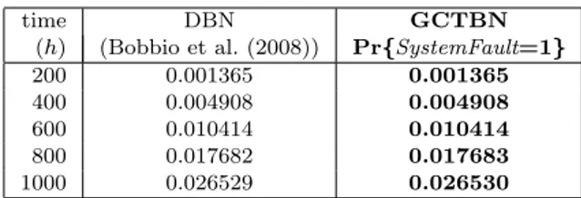
(h) (Bobbio et al. (2008)) Pr{SystemFault=1} 200 0.001365 0.001365 400 0.004908 0.004908 600 0.010414 0.010414 800 0.017682 0.017683 1000 0.026529 0.026530 4.1 Unreliability analysis

In order to compute the system unreliability (the prob-ability to be failed at a given time), it is sufficient to query the variable SystemFault in the GCTBN (Fig. 4), at the desired time points, given no evidence. The system unreliability has been evaluated up to 1000 h (Tab. 3). In Bobbio et al. (2008) the same measure is computed by analyzing the DBN (Fig. 3) by means of the software tool Radyban (Portinale et al. (2007)). There is an almost complete agreement among the results (Tab. 3). In partic-ular, the DBN is a discrete time model (Sec. 2.2), and a time discretization step ∆=1 h is assumed.

Differently from standard (D)FT analysis, it is possible to query in a contemporary way, any other variable in the model: Tab. 4 reports the unreliability of the three sub-systems, obtained by querying the variables SensorFault, DigCon, and PumpFault.

SAFEPROCESS 2015

September 2-4, 2015. Paris, France

(4)

Fig. 1. The block scheme of HSS (Bobbio et al. (2008)) Table 1. The component failure rates (λ)

Component λ Component λ

Sensor 10−4_h−1 _Pump ₁₀−6_h−1

VF 10−5_h−1 _DigCon ₁₀−6_h−1

Fig. 2. DFT model of HSS (Bobbio et al. (2008))

cases, SensorFault is equal to 0. This is set in the CPT of SensorFault and corresponds to the 2:3 gate in the DFT. The immediate variable Pump1Fault indicates whether the primary pump is functioning or not, and is influenced by the causes of malfunctioning: Pump1 (the failure of the pump) or VF1 (the failure of the valve/filter). Pump2Fault has the same role with respect to the secondary pump. The delayed variable Pump2 concerns the state of the backup pump which is activated in case of malfunctioning of the primary pump; so, Pump2 depends on Pump1Fault. As a consequence, the rates inside the CIM of Pump2 depend on the value of Pump1Fault, as reported in Tab. 2. Pump2 is a “cold” spare (Sec. 2.1): if Pump1Fault is equal to 0, then the transition rate of Pump2 from 0 to 1 is null; if instead Pump1Fault is equal to 1, the rate of Pump2 from 0 to 1 is the failure rate of the pump (Tab. 1). The transition rate from 1 to 0 is null in both cases because Pump2 is not repairable.

The immediate variable PumpFault is equal to 1 when both Pump1Fault and Pump2Fault are equal to 1. In all the other cases, PumpFault is equal to 0, as specified in its CPT. Finally, the immediate variable SystemFault corresponds to the top event of the DFT, and its CPT realizes the OR gate.

4. ANALYSIS OF THE CASE STUDY

We can perform relevant evaluations in a reliability setting by exploiting an inference engine for GCTBN (Codetta and Portinale (2013)), developed inside the Draw-Net modeling software tool (Codetta et al. (2006)).

Fig. 3. DBN model of HSS (Bobbio et al. (2008))

Fig. 4. GCTBN model of HSS

Table 2. CIM of the variable Pump2

0→ 1 1→ 0 Pump1Fault rate Pump1Fault rate

0 0 0 0

1 10−6h−1 1 0

Table 3. System unreliability (no evidence)

time DBN GCTBN

(h) (Bobbio et al. (2008)) Pr{SystemFault=1} 200 0.001365 0.001365 400 0.004908 0.004908 600 0.010414 0.010414 800 0.017682 0.017683 1000 0.026529 0.026530 4.1 Unreliability analysis

In order to compute the system unreliability (the prob-ability to be failed at a given time), it is sufficient to query the variable SystemFault in the GCTBN (Fig. 4), at the desired time points, given no evidence. The system unreliability has been evaluated up to 1000 h (Tab. 3). In Bobbio et al. (2008) the same measure is computed by analyzing the DBN (Fig. 3) by means of the software tool Radyban (Portinale et al. (2007)). There is an almost complete agreement among the results (Tab. 3). In partic-ular, the DBN is a discrete time model (Sec. 2.2), and a time discretization step ∆=1 h is assumed.

Differently from standard (D)FT analysis, it is possible to query in a contemporary way, any other variable in the model: Tab. 4 reports the unreliability of the three sub-systems, obtained by querying the variables SensorFault, DigCon, and PumpFault.

Table 4. Subsystem unreliability (no evidence)

time Sensor set Controller Pump set

(h) Pr{SensorFault=1} Pr{DigCon=1} Pr{PumpFault=1}

200 0.001161 0.000200 0.000005 400 0.004492 0.000400 0.000018 600 0.009779 0.000600 0.000041 800 0.016824 0.000800 0.000073 1000 0.025444 0.001000 0.000114

Table 5. The system unreliability conditioned on σ1(monitoring task)

time DBN GCTBN

(h) (Bobbio et al. (2008)) Pr{SystemFault=1 | σ1}

100 0.000200 0.000200 200 0.000402 0.000401 300 0.000604 0.000604 400 0.000808 0.000807 500 0.058733 0.058750 600− 1000 1.000000 1.000000

GCTBN offer the possibility of performing computations conditioned on the observation of some system parameters. Let us suppose that Sensor2 and Sensor3 can be monitored in HSS. Let St

i be the observation that the i-th sensor is down at time t, and let St

i be the observation that the i-th sensor is up at t. We get the following stream of observations: σ1= {S 100 2 ; S 200 3 ; S 300 2 ; S 400 3 ; S2500; S3600} (1)

In order to compute the system unreliability conditioned on σ1, we have to associate the evidence with the variables

Sensor2 and Sensor3; then, the GCTBN monitoring task from time 100 h to 1000 h is performed, still querying SystemFault. The results are shown in Tab. 5, together with the corresponding values returned by DBN analy-sis (Bobbio et al. (2008)); we can notice that GCTBN and DBN still provide coherent results. This holds also in the case of smoothing: at time 100 h, the unreliability given by both GCTBN and DBN inference is equal to 0.000101. The monitoring unreliability is larger than the smoothing unreliability, since the smoothing procedure takes into account the future information about the operative state of the sensors. At time t=100 h, the monitoring unreliability is the probability of having a system failure, given that we know that Sensor2 is operational at t. The smoothing unreliability instead, at t=100 h provides the probability that the whole system is down at t, knowing not only the sensors history until t, but also the following sensors history. From σ1we know that at times 100 h, 200 h, and

300 h, Sensor2 and Sensor3 are still operational. So, at 100 h the smoothing task knows for sure that also Sensor3 is operative. As a consequence, the probability of system failure is reduced.

4.2 Diagnosis

Another possibility consists in performing a diagnosis over the status of the components, given a stream of observations. Let us consider to gather information about the global state of the system, and suppose to get the following stream of observations (where SF stands for SystemFault):

σ2= {SF 200

; SF400; SF600

} (2)

Table 6. Component failure probability condi-tioned on σ2(monitoring)

time DBN monitoring (Bobbio et al. (2008)) (h) Sensor DigCon VF Pump1 Pump2 100 0.009950 0.000100 0.000999 0.001099 0.000999 200 0.019047 0.000000 0.001994 0.002193 0.001994 300 0.028808 0.000010 0.002991 0.003290 0.002991 400 0.036359 0.000000 0.003975 0.004372 0.003974 500 0.045948 0.000010 0.004971 0.005467 0.004971 600 0.645037 0.036144 0.009686 0.010651 0.010060 700 0.648568 0.036241 0.010676 0.011739 0.011050 800 0.652065 0.036337 0.011664 0.012826 0.012039 1000 0.658955 0.036529 0.013639 0.014995 0.014015 time GCTBN monitoring

(h) Sensor1 DigCon VF1 Pump1F. Pump2F.

100 0.009950 0.000100 0.001000 0.001099 0.001000 200 0.019047 0.000000 0.001994 0.002193 0.001994 300 0.028808 0.000100 0.002992 0.003290 0.002992 400 0.036389 0.000000 0.003973 0.004368 0.003973 500 0.045977 0.000100 0.004969 0.005463 0.004969 600 0.648770 0.037545 0.011449 0.012562 0.011823 700 0.652265 0.037641 0.012437 0.013647 0.012812 800 0.655725 0.037737 0.013424 0.014732 0.013800 1000 0.662542 0.037930 0.015395 0.016897 0.015773

Table 7. Component failure probability condi-tioned on σ2(smoothing)

time DBN smoothing (Bobbio et al. (2008)) (h) Sensor DigCon VF Pump1 Pump2 100 0.065745 0.000000 0.001384 0.001522 0.001384 200 0.130836 0.000000 0.002767 0.003044 0.002767 time GCTBN smoothing

(h) Sensor1 DigCon VF1 Pump1F. Pump2F.

100 0.067859 0.000000 0.001398 0.001539 0.001400 200 0.134236 0.000000 0.002799 0.003083 0.002801

This means that the system has failed in the interval (400, 600]. We can ask for the failure probability of the components, given σ2. To this end, we associate σ2 with

SystemFault, and we query the variables modeling the components. In particular, the pumps have been evaluated with respect to the variables Pump1Fault and Pump2Fault representing the operational or malfunctioning condition according to the state of the pumps and the state of their support streams (Sec. 3.2). Results returned by GCTBN inference are reported in Tab. 6 (monitoring) and in Tab. 7 (smoothing), where we notice that they are quite similar to those obtained by means of DBN analysis (Bobbio et al. (2008)). The differences are due to the different temporal dimensions; in particular, the discrete time in DBN may lead to some approximation (Sec. 5).

By analyzing the smoothing results (Tab. 7), we can notice that the digital controller (DigCon) cannot be failed at times 100 h and 200 h; this is consistent with the fact that a failure of such a component will cause a system failure (see the DFT in Fig. 2) and that we have observed the system being operational until time 400 h. This is not reported in the monitoring analysis (Tab. 6), where DigCon can be assumed operational only at the times when we gather the information about the system being up (i.e. 200 h and 400 h); for the other times before 400 h, the monitoring analysis predicts a possibility of failure for DigCon.

(5)

680 Daniele Codetta-Raiteri et al. / IFAC-PapersOnLine 48-21 (2015) 676–681

Table 8. Importance indices of components

Component Fussell-Vesely index (FVI) Birnbaum index (BI)

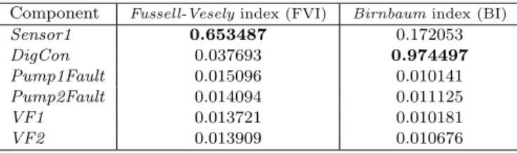
Sensor1 0.653487 0.172053 DigCon 0.037693 0.974497 Pump1Fault 0.015096 0.010141 Pump2Fault 0.014094 0.011125 VF1 0.013721 0.010181 VF2 0.013909 0.010676 4.3 Importance indices

Two relevant importance (sensitivity) indices adopted in reliability analysis are the Fussell-Vesely Importance (FVI) and the Birnbaum Importance (BI) (Meng (2000)). They are aimed at determining the importance of each component in the event of a system failure. FVI of a generic component C is defined as the probability of C being failed, given that the system is failed. BI of C instead, measures the change in the system unreliability, given that C is down (SF stands for SystemFault):

F V I(C) = P r(C = 1_{|SF = 1)} (3) BI(C) = P r(SF = 1|C = 1) − P r(SF = 1|C = 0) (4) Both indices are a simple matter of posterior probability computation for a GCTBN. Tab. 8 shows FVI and BI of the components in the case study, computed at time 1000 h. We can notice that FVI clearly suggests the sensor as the most relevant component w.r.t. the occurrence of the system failure: actually the sensor has the highest failure rate (Tab. 1), and the system is tolerant to the failure of only one sensor, as modelled by the 2:3 gate in the DFT model (Fig. 2). On the other hand, BI points out that the controller is the most important from the point of view of the change of unreliability; indeed, the controller is a direct cause of the system failure.

4.4 Repair and unavailability

Since components are represented in a GCTBN as delayed variables, a repairable component can be modeled by in-troducing a suitable repair rate in the CIM of the corre-sponding variable. As an example, now we suppose that in HSS the following components are repairable: two of the three sensors, the digital controller, the primary pump, and its support stream. The repair rate is µ=0.01 h−1 for every component. In the GCTBN model, µ becomes the transition rate from the value 1 (failed) to the value 0 (working) for the following variables: Sensor1, Sensor2, DigCon, Pump1, and VF1.

Tab. 9 shows the subsystem and the system unavailability (probability to be down at a certain time) from 100 h to 1000 h, assuming that no evidence is observed. We can notice an evident reduction of the probability to be down, with respect to the results obtained without repair (Tab. 3 and Tab. 4). Using GCTBN we can compute the steady-state unavailability (unavailability at an infinite time) which indicates whether the (sub)system is dependable in the long run. The results are still reported in Tab. 9. GCTBN can be exploited to model more sophisticated repair policies like those involving a subsystem instead of a single component (Portinale et al. (2010)).

Table 9. Unavailability (no evidence)

time (h) Sensor set Controller Pump set System 200 0.000411 0.000086 0.000002 0.000499 400 0.000850 0.000098 0.000004 0.000952 600 0.001199 0.000100 0.000006 0.001305 800 0.001569 0.000100 0.000009 0.001677 1000 0.001928 0.000100 0.000011 0.002039 ∞ 0.019704 0.000100 0.001099 0.020879 5. COMPARING GCTBN AND DBN

We compare the DBN and the GCTBN formalism from several points of view, with the goal of showing the advantages of GCTBN modeling and analysis.

5.1 Modeling

The introduction of time evolving parts is clearly possible in DBN, where the two instances of the variables hav-ing a temporal evolution are connected by temporal arcs (Sec. 2.2). This leads to a duplication of the nodes concern-ing such variables. An example is shown in Fig. 3 where the nodes representing the states of the components (Sensor1, Sensor2, Sensor3, DigCon, Pump1, Pump2, VF1, VF2) are present in both time slices (t − ∆ and t). GCTBN instead, provide a more compact representation because variables are never replicated, as shown in Fig. 4.

The design of a DBN model requires to set all the entries of the CPT of each node. The entries are as many as the possible combinations of the node values and the parent node values, including the historical copies. In GCTBN, delayed nodes (having a temporal evolution) do not depend on their historical copies, so the number of entries in their CIM is reduced with respect to the corresponding CPT in the DBN.

The CIM entries are simply set to transition rates, such as failure or repair rates. In a DBN instead, in the time slice t, the CPT entries of a time-evolving variable are probabilities to be pre-computed during the model design according to the failure or repair rate of the component and the time discretization step.

5.2 Temporal dimension

DBN is a discrete time formalism, so a time discretization step (∆) must be set. When the inference is performed, all the intervening time steps from 0 to the query time, have to be dealt with, even if no evidence is available at a certain time step. Therefore ∆ rules the computing time and the precision of the results; it is worth noting that a trade-off exists: if a looser approximation is sufficient, a quicker DBN inference can be obtained, by choosing a relatively large ∆; if instead we apply a smaller ∆, then the DBN is closer to a continuous time model, the accuracy of the results is improved, but the computing time grows. However there is not always an obvious discrete time unit: when the process is characterized by several components evolving at different rates, the finer granularity dictates the rules for the discretization (Portinale et al. (2007)). Moreover, variables can be observed or queried only at specific time steps according to ∆.

GCTBN has no need for time discretization; as a conse-quence, the model designer has not to choose a proper SAFEPROCESS 2015

September 2-4, 2015. Paris, France