_____________________________________________________________________________________________________
*Corresponding author: E-mail: [email protected];
(Past name:American Journal of Experimental Agriculture,Past ISSN: 2231-0606)
Irrigation Scheduling Optimisation in Olive Groves
A. Capra
1*and B. Scicolone
11Department of Agraria, Mediterranean University of Reggio Calabria, Località Vito, 89060 Reggio
Calabria, Italy. Authors’ contributions This work was carried out in collaboration between both authors. Article Information
DOI: 10.9734/JEAI/2018/44582
Editor(s):
(1)Dr. Marco Aurelio Cristancho, Professor, National Center for Coffee Research, CENICAFÉ, Colombia. (2) Dr. Mohammad Reza Naroui Rad, Department of Seed and Plant improvement, Sistan Agricultural and Natural Resources
Research Center, AREEO, Zabol, Iran.
Reviewers:
(1) Alexandra Tomaz, Instituto Politécnico de Beja, Portugal. (2) Raúl Leonel Grijalva-Contreras, Instituto Nacional de Investigaciones Forestales Agrícolas y Pecuarias, México. (3) W. James Grichar, Texas A & M University Research, USA. (4) Miguel Aguilar Cortes, Universidad Autonoma Del Estado De Morelos, Mexico. Complete Peer review History: http://www.sciencedomain.org/review-history/27281
Received 19 September 2018 Accepted 13 November 2018 Published 17 November 2018
ABSTRACT
Introduction: The diffusion of irrigation in olive orchards requires accurate scheduling of the application of water.
Objectives: To evaluate the efficiency of different modes of irrigation scheduling for mature olive trees grown at different plant densities and in different soil types and irrigated under different systems and strategies.
Methodology: We compare the irrigation scheduling with variable quantities and intervals (OPT), optimised by the water balance-evapotranspiration method (WB-ET) by evaluating the use of variable quantities and different fixed intervals (3, 7, 14 and 28 days) as well as a fixed interval and quantity (FIX). These scheduling scenarios were applied to high-density and super-high density groves in medium to fine textured and moderately coarse to medium textured soils irrigated by sprinkler, microjets and drip irrigation systems under full and deficit (sustained, SDI and regulated, RDI) irrigation strategies in a Mediterranean environment (Calabria Region, Italy). Three sets of measured meteorological data (2016, 2017 and the mean values of the 2001-2017) were used for simulations.
Results: OPT scheduling showed maximum efficiency. Three-day and weekly intervals show acceptable performance in terms of efficiency as well as water and energy requirements, whereas
FIX scheduling shows very low efficiency. SDI and RDI permit mean savings of approximately 36%-54% of water and energy compared to full irrigation. High-density orchards drip irrigated under the SDI strategy show minimum water and energy requirements.
Conclusions: The traditional irrigation strategy at fixed quantity and interval is not adequate to achieve high efficiency in the irrigation of olive orchards, from both the agronomic (reduction of crop water stress) and economic (reduction of water and energy requirements) point of view. The optimisation of the irrigation scheduling requires the estimate of the water quantity to deliver in each irrigation in both the irrigation management at variable and fixed interval. The WB-ET model is an efficient and (relatively) simple tool to foresee the quantities and the dates of irrigation during the irrigation season.
Keywords: Energy irrigation requirements; evapotranspiration; irrigation efficiency; irrigation scheduling; olive orchards; water balance.
1. INTRODUCTION
Olive trees are among the most important and common plants in the Mediterranean basin. Although this species (Olea europaea L.) has been traditionally cultivated under rainfall conditions, irrigation also plays an important role, especially in soils with limited water storage to stabilise yields in years of low rainfall [1,2,3,4,5]. In particular, irrigation is needed in new orchards planted at very high densities (1000-2000 trees/ha) [3,6].
However, olive-growing areas are often located in arid or semi-arid regions where water reservoirs are already highly exploited and the development of new water resources is not economically or environmentally viable [7,8]. Improving irrigation efficiency and applying deficit irrigation are the main strategies to save water. Due to the reduction of soil evaporation and deep losses, localised irrigation systems are potentially able to achieve high efficiencies [9,10,11]. Deficit irrigation strategies (DI), such as the application of irrigation in quantities below total crop evapotranspiration (ETc), are potentially
able to improve efficiency and maximise profits in several crops [12]. The literature describes a variety of DI strategies [13,14]. Experiments examining two main strategies have been conducted in olive groves: regulated deficit irrigation (RDI) and sustained deficit irrigation (SDI) [6,14,15,16,17,18]. Under RDI, quantities of water close to ETc are applied at the
phenological stages most sensitive to water stress, while irrigation is reduced, or even interrupted, for the rest of the growing season. Under SDI, a deficit is applied throughout the season. Recent evidence has shown that the qualitative characteristics of olives and the
profitability of super high density (SHD) olive orchards can be optimised using DI strategies [3,19,20,21,22].
However, the adoption of localised systems together with DI is not a guarantee of success. Only well-designed and well-managed irrigation systems can ensure high efficiency [10,11,23]. In particular, in irrigation management, significant improvements can be achieved through the proper scheduling of irrigation [8,24].
The most common definition of irrigation scheduling simply involves two questions: when and how much to irrigate a crop [25,26]. The four main methods informing an appropriate irrigation schedule rely on evapotranspiration (ET) and
water balance (ET-WB), soil tension or soil moisture along the rooting depth,
measurements of plant stress, and simulation models [27,28,29].
Although there is a wide body of literature on scientific irrigation scheduling in reference works, journal articles, symposium proceedings and extension publications, irrigators generally do not adopt effective methods [8,25,27,30]. Due to the need for substantial investments in management capacity as well as in improving or replacing irrigation systems, the majority of growers worldwide still manage irrigation applications based on rigid calendars determined by external factors [26,31]. There is a difference in the approach to irrigation scheduling between farmers and scientists. Scientists depict irrigation scheduling as an accurate process, with the timing of irrigation being defined as a precise date or time, while from a practical point of view, irrigation scheduling sometimes needs to be adjusted in association with many other farm activities and based on constraints [32]. Furthermore, in olive orchards, water irrigation
doses and frequencies seem to influence the development of Verticillium wilt [33,34]. Despite a significant lack of information about the influence of irrigation management on the diffusion of this disease [35], low frequency irrigation is recommended [3].
The types of irrigation that are scheduling-applicable in practice are as follows: i. irrigation with variable intervals and quantities of water; ii. irrigation with a fixed interval and variable quantities of water; and iii. irrigation with a fixed interval and a fixed quantity of water. The first type requires that water is available upon demand in terms of both quantities and intervals. Scheduling with a fixed interval and variable quantities requires that water is available upon demand for quantities but not for interval, which can simplify irrigation management. Most farmers prefer the third method because it is easy to manage. Furthermore, this method is the most common in areas supplied with collective irrigation systems.
The objective of the present work is to evaluate the efficiency of different modes of irrigation scheduling for mature olive trees grown at different plant densities and in different soil types and irrigated under different systems and strategies. The study mainly uses data from an important Mediterranean area for oil production, the Calabria Region in Italy, but also analyses other conditions that are not widespread in the area to allow the results to be generalised for the Mediterranean environment. The general aim of the study is to enable producers to apply appropriate irrigation practices to olive, a crop with a relatively recent history of irrigation. 2. MATERIALS AND METHODS 2.1 Data Used for Simulations
Different combinations of meteorological data, growing systems, soil types, and irrigation strategies and systems were considered to test the efficiency of irrigation scheduling.
The following cases were considered (Table 1): Three sets of meteorological data: for 2016, 2017, and the mean values of the 2001-2017 period;
Two growing systems: high density (HD) and
super-high-density (SHD) groves;
Two soil types: medium to fine texture (sandy clay loam, loam, silty loam, clay loam to silty clay loam), with a high water-holding capacity (Fsoil); and moderately coarse to medium texture (sandy loam to fine sandy loam, sandy clay loam, loam, silty loam), with an intermediate water-holding capacity (Msoil);
Three types of irrigation strategies: full irrigation (100% ETc, Full); RDI 50% ETc, with the deficit
concentrated in the summer period, from pit hardening until the end of the summer [9,11]; and SDI 50% ETc, with the deficit distributed evenly
throughout the irrigation season;
Three types of irrigation system; a sprinkler system (SIS), localised irrigation with microjets (MIS) and localised irrigation with drippers (DIS).
The meteorological, soil and crop data came from an Italian area of particular importance for oil production. The area considered is located in Lametia in the Calabria region. Calabria is the second largest producer of olive oil in Italy, accounting for almost one-third of national production [36]. The characteristics of the irrigation systems considered in this study are standard for well-designed and well-managed irrigation systems for cultivated olives [9,11]. The SHD growing system, the SDI and the RDI irrigation strategies, and the sprinkler irrigation system were added to the simulation to allow the results of this study to be generalised, despite not being widespread in the study area. For the same reason, the simulations were replicated for the three series of meteorological data.
2.2 Estimation of Irrigation Requirements Irrigation requirements were estimated using a daily soil water balance model (WB), implemented in a spreadsheet, specifically developed during this study. In the WB method, an estimate of evapotranspiration (ET) coupled with the WB equation enables the calculation of the soil water deficit, which is then compared with the readily available water in the soil (RAW). When water depletion exceeds RAW, an irrigation event returns the soil water content (θ) to field capacity (θFC).
The water balance ET based method (WB-ET) is a well-established, simple, robust method [37] with a long history [38]. For this reason, we describe only the main concepts and the specific assumptions applied in this study.
According to Allen et al. [38], the equation for daily soil WB is as follows:
Dr,i = Dr,i−1 − (P − RO)i − Inet,i − CRi + ETc,i +
DPi (1)
where D (mm) is the depletion of water from the root zone; i is the current day; i − 1 is the previous day; P (mm) is daily precipitation; RO (mm) is the runoff; Inet (mm) is the net irrigation
depth; CR (mm) is the capillary rise from the groundwater table; ETc (mm) is the crop
evapotranspiration; and DP (mm) is the deep percolation.
Considering the conditions inherent to the crop and the area examined and the objective of the study, we assumed the following:
The quantity of rainfall stored in the root zone (P-RO-DP)i can be represented by the effective
rainfall, Pe (mm); for the estimation of Pe, P< 0.3
mm was ignored, while RO was considered
negligible, and DP was considered negligible when the soil water content in the root
zone was below θFC and was considered equal to
P-θFC when the soil water content was higher
than θFC;
CR was considered negligible (the depth of the water table is greater than 5 m);
ETc was calculated as follows:
ETc = ET0 x Kc (2)
where ET0 is the reference evapotranspiration
estimated according to the FAO Penman-Montieth equation, and Kc is the crop coefficient
[38];
Two other coefficients, a coefficient of localisation (Kl) and a stress coefficient (Ks),
were used to adjust equation (2) for localised irrigation systems and deficit irrigation strategies, respectively; equation (2) was therefore modified as follows:
ETc = ET0 x Kc x Kl x Ks (2a)
The value used for Kc was 0.65 until the end of
May and 0.55 from June onward [3].
The coefficient of localisation Kl was estimated
as [9]:
Kl=Pc/100+0.5*(1-Pc/100) (3)
where Pc= mean ground coverage by canopy (%)
measured in the field.
The values for the stress coefficients (Ks) (see
Table 1) where established according to the irrigation strategy simulated (full irrigation, RDI and SDI).
RO for irrigation water was considered negligible, and DP was accounted for by the potential irrigation system efficiency (PAE, % [42]); Inet
was therefore replaced by Igross, which was
estimated as Inet/(PAE/100).
These assumptions simplify equation (1) as follows:
Dr,i = Dr,i−1 − Pei − Igross + ETc,i (1a)
The total available water (TAW) is the quantity of water stored in the root zone that a plant can utilise and is calculated as follows
[38]:
TAW = (θFC − θPWP) × Z (4)
Where θFC is the field capacity (mm/m); θPWP is
the permanent wilting point (mm/m); and Z is the root zone depth (m).
To prevent permanent physiological damage to the crop, irrigation is usually applied before the soil water content is equal to θPWP. The fraction
of TAW that a crop can extract without suffering water stress is the readily available soil water (RAW)
= (5)
where p is the average fraction of TAW that is depleted before moisture stress and is equal to 0.65 for olives [38]; and Sw is the wetted surface
area (%), which was equal to 100% in SIS and was below 100% for the localised systems (MIS and DIS).
Table 1 shows the values used in this study for PAE, θFC, θPWP, Z and Sw.
The hydrological characteristics of the soils were estimated by pedotransfer functions based on sand, silt, clay and organic carbon soil contents and on bulk density using the software SOILPAR 2.00 [39]. The Calabria soil map [40] was overlapped to the land use map [41] by a GIS to identify the soil types, and their physical-chemical characteristics, in the areas cultivated with the crop of interest in the agricultural areas observed.
5
Table 1. Variables used in the simulations for the different types of soil, growing systems (plant density), irrigation systems and irrigation strategies
Soil type Field capacity
(θFC,mm/m) Permanent wilting point (θPWP, mm/m) Readly available water (RAW, mm/m) Wetted width(1) (m)
1 Medium to fine texture, high water holding capacity (Fsoil) 300 170 84 0.8
2 Moderately coarse to medium texture, medium water holding capacity (Msoil)
200 100 65 0.6
Plant density Plant age
(years)
Root depth (Z, m)
Plant spacing in the row (m)
Row spacing (m) Ground coverage by canopy (%)
1 High density (HD) (286 trees/ha)[3] 15 0.8 5 7 45
2 Super high density (SHD) (1667 trees/ha) [3]
4 0.6 1.5 4 82
Irrigation system Mean number of
emission point per plant
Wetted surface (Sw, %) Emitter characteristics
HD SHD HD SHD mean discharge (L/h) working pressur
head (kPa) 1 Sprinkle (SIS) (PAE(2)= 80%
[9, 39]
0.25 0.06 100 100 1080 300
2 Microjets (single lateral system) (MIS)(PAE(2)= 85%)[9,39]
Fsoil 1 1 32.4 100 75 150
Msoil 1 1 29.1 88.5 75 150
3 Drip (double lateral system) (DIS)(PAE(2)= 90%)[9,39]
Fsoil 7.7 2.3 22.1 36.7 4 100
Msoil 10 3 16.2 28.3 4 100
Irrigation strategy Coefficient of stress Ks
until June, 30th after June
1 Full irrigation, 100% Etc (Full) 1 1
2 Regulated deficit irrigation, with deficit (50% Etc) concentrated in the summer period, from pit
hardening until the end of the summer season (RDI)
1 0.5
3 Sustained deficit irrigation, 50% ETc, with deficit distributed evenly throughout the whole irrigation
season (SDI)
0.5 0.5
(1)
Considering the Mediterranean climate, the WB-ET model was run from April 1st to October
31th.
2.3 Irrigation Scheduling
In this study, we define “optimal irrigation scheduling” as irrigation management that ensures that irrigation is applied at the time when RAW is depleted (Dr,i <RAW). This type of
scheduling, which implies variable intervals and quantities of water, is “optimal” from both the agronomic (no water stress in the crop) and the hydrological (no water losses beyond that considered by PAE, due to deep percolation) points of view. In contrast, irrigation management at fixed intervals and variable water quantities or at fixed intervals and water quantities may not achieve high efficiency.
Six different types of irrigation scheduling were simulated in this study: (a) optimal irrigation scheduling (OPT), (b) irrigation at three days intervals and variable quantities (three days), (c) irrigation at weekly intervals and variable quantities (weekly), (d) irrigation at 14 days intervals and variable quantities (14 days), (e) irrigation at 28 days intervals and variable quantities (28 days) and (f) irrigation with a fixed interval and quantity (FIX).
Both the water quantity and irrigation dates for scheduling type (a) and only the quantity of water for cases (b) to (e) were established based on the WB-ET method.
For strategy (f), the fixed quantity of water was determined by using the RAW corrected by the irrigation system efficiency (PAE):
=
/ (5)
The fixed interval (F) was obtained as follows:
F = ISlm/IrriN (6)
IrriN =WRs/RAWg (7)
where F is the fixed irrigation interval (days); ISl
is the irrigation season length, which is defined as the total number of days between the first and last irrigation event in a year (days); IrriN is the total number of irrigation events in the season; WRs is the gross seasonal water requirement
(mm); and RAWg is the gross readily available
water (mm).
ISlm was fixed at approximately 110 days
because the farmers, in the area examined, generally irrigate their olive orchards from mid-June to September. WRs was calculated based
on the mean values of ET0 and P estimated from
the climatic data measured by a meteorological station located near the study area over the period from 1925-2017. The values calculated for WRs were 241, 227 and 215 mm for SIS, MIS
and DIS, respectively.
Approximately 650 simulations, derived from the combination of the numbers of scheduling modes, growing systems, soil types, irrigation strategies, irrigation systems and meteorological datasets, were therefore performed and analysed.
2.4 Irrigation Management Efficiency To determine the efficiency of water application, the results of the simulations for 3, 7, 14 and 28 days intervals and FIX irrigation scheduling were compared to those for OPT scheduling. With this aim, in addition to the gross irrigation (Igross, mm),
the total number of irrigation events (IrriN) applied over the irrigation season and the
irrigation season length (ISl, days), the
following indices were calculated and are discussed:
Total energy applied; Irrigation adequacy; Scheduling efficiency.
The total energy applied was estimated as follows:
=
(8)
where Ener is the total energy applied (kWh/ha); Q is the system discharge (L/s); H is the total operating head (m); Ep is the engine pump
efficiency (decimal); 102 is the conversion constant; and Id is the total time of irrigation in
the irrigation season (h/ha).
The irrigation adequacy (IA) quantifies the ability of irrigation management to supply
sufficient irrigation to meet plant water demands without stress [43, 44]. We distinguished two types of stress: light stress, which occurs when the soil moisture content is lower than RAW but higher than θPWP, and severe stress, which
occurs when the soil moisture content is below θPWP.
Three indices were used to evaluate IA:
(9)
(10)
(11)
where IA1 (%) represents the days of the
irrigation season without any stress (both light and severe) in fully irrigated plants; IA2 (%)
represents the days of the irrigation season without severe stress in fully irrigated plants; IA3
(%) represents the days of the irrigation season without extra stress beyond that specified in the deficit irrigation strategy (RDI or SDI); ISl (days)
is the length of the irrigation season; DST (days)
is the total number of crop stress days (sum of light and severe stress days); DSS is the number
of severe crop stress days; and DSe is the
number of stress days beyond those due to the deficit irrigation strategy (RDI or SDI).
The scheduling efficiency (SchE) is defined as the ability of a management method to achieve irrigation without drainage or runoff (similar to the SWAT procedure described by [43]). The SchE index represents the percentage of the total gross irrigation retained in the root zone and is calculated in the irrigation season with the following equation:
(12)
where SchE (%) is the scheduling efficiency index; Igross (mm) is the sum of gross irrigation
applied over the irrigation season; and Surplus (mm) is the depth of water above the field capacity leading to deep percolation (runoff was assumed to be zero due to the effectively designed irrigation systems).
3. RESULTS AND DISCUSSION 3.1 Meteorological Characteristics
The maximum (Tmax) and minimum (Tmin) temperatures during the period from April 1st to October 31st were approximately 25°C and 17°C,
respectively (mean of the three datasets). Tmax and Tmin showed higher values in 2017 (37.5°C) and for the mean period (approximately 10°C), respectively, while lower values were observed in 2016 for Tmax (14.6°C) and in 2017 for Tmin (2.8°C) (Figures 1 a, b, c). Tmin showed higher variability than Tmax, with coefficients of variation (CV) of 22, 29 and 20% for the 2016, 2017 and 2001-2017 datasets, respectively. The corresponding values of CV for Tmax were 14, 17 and 14%.
Precipitation was the most variable
characteristic, with total precipitation of 457, 193 and 325 mm being observed for the 2016, 2017 and 2001-2017 datasets, respectively. Exceptionally high daily precipitation (61.7 mm) was recorded in 2016 (Fig. 1a).
The daily mean values of ET0 ranged from 3.50
mm (in 2001-2017 dataset) to 4.56 mm (in 2016); the corresponding values of accumulated ET0
from April to October were 750 mm (2001-2017) and 956 mm (2016). As expected for the
environment examined [45], the average values (2001-2017) showed an upward trend of
ET0 up to July and then a decreasing trend.
Between the two individual years considered, 2016 exhibited a normal trend of ET0, while in
2017, peaks of ET0 were recorded in the second
half of June.
3.2 Optimal Irrigation Scheduling
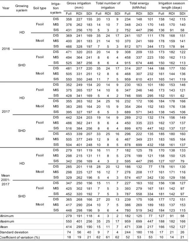
The gross irrigation applied over the irrigation season (Igross) ranged between 279 and
550 mm for full irrigation and was 191-401 and 118-256 mm for the RDI and SDI deficit strategies, respectively (Table 2). CV
between the different hypothesised conditions was approximately 20% for the full irrigation,
RDI and SDI strategies (Table 2). The total energy applied over the irrigation season
varied between 182 and 959 kWh/ha for full
irrigation (Table 2). The energy savings assured by the deficit strategies were of the
same order of magnitude described for Igross (40% for RDI, 113% for SDI, and 53% for
SDI with respect to RDI). The coefficient of
variation of approximately 50% is higher than Igross due to the influence of the
irrigation duration and the number of irrigation events in the season (IrriN) on energy consumption.
100 1 x IS DS IS IA l T l
100 2 x IS DS IS IA l S l
100 3 x IS DS IS IA l e l
100 x I Surplus I SchE gross gross Fig. 1. Meteorological characteristics of the S. Eufemia Lametia (Calabria, Italy) station (a=2016; b= 2017; c= mean 2001-2017) (P= precipitation; ETo= reference evapotranspiration;
Tmax= maximum temperature; Tmin= minimum temperature) Due to the different irrigation systems
considered, the total number of irrigation events in the irrigation season (IrriN) is the most variable parameter (CV of approximately 60%). On average, IrriN ranged from 11 to 24 irrigation events for drip systems (DIS), from 6 to 13 for microjet systems (MIS), and from 3 to 7 for sprinkler systems (SIS) (Table 2). Among the different irrigation strategies, the lowest values
corresponded to SDI, followed by RDI, and the highest corresponded to full irrigation.
The mean irrigation season length (ISl) was 166,
152 and 127 days for the full, RDI and SDI systems, respectively (Table 2). The corresponding CV values were 10, 14 and 21% (Table 2). 0 5 10 15 20 25 30 35 40 0 10 20 30 40 50 60 70 4/1 4/8 54/1 4/22 4/29 5/6 5/13 0/25 75/2 6/3 6/10 6/17 6/24 7/1 7/8 57/1 7/22 7/29 8/5 8/12 8/19 6/28 9/2 9/9 9/16 9/23 9/30 10/7 1 0/ 1 4 1 0/ 2 1 1 0/ 2 8 Tmax, Tmin (° C) P , Eto (m m) (a) P ETo Tmax Tmin 0 5 10 15 20 25 30 35 40 0 10 20 30 40 50 60 70 4/1 4/8 4/15 4/22 4/29 5/6 5/13 5/20 5/27 6/3 6/10 6/17 6/24 7/1 7/8 7/15 7/22 7/29 8/5 8/12 8/19 68/2 9/2 9/9 9/16 9/23 9/30 10/7 10 /14 10 /21 10 /28 Tm ax , T min (° C) P, Eto (m m ) (b) P ETo Tmax Tmin 0 5 10 15 20 25 30 35 40 0 10 20 30 40 50 60 70 4/1 4/8 4/15 4/22 4/29 5/6 5/13 05/2 5/27 6/3 6/10 6/17 6/24 7/1 7/8 7/15 7/22 7/29 8/5 8/12 8/19 8/26 9/2 9/9 9/16 9/23 9/30 10/7 10 /14 10 /21 10 /28 Tm ax , T min (° C) P, Eto (m m ) (c) P ETo Tmax Tmin
The date of the first irrigation event varied from April 22nd to May 2nd for both full and RDI irrigation (under RDI, the deficit was applied starting in July) and from May 14th to May 29th for SDI (data not shown). Irrigation generally ended in September or October (data not shown). Due to the different irrigation system efficiencies (PAE in Table 1), both Igross and Ener were, as
expected, highest in SIS, followed by MIS, and they were lowest in DIS (Table 2). DIS required approximately 10% (1-18%) and 19% (9-40%) less water and 37% (30-42%) and 52% (43-66%) less energy on average than MIS and SIS, respectively.
On the other hand, the total number of irrigation events (IrriN) and the irrigation season length (ISl) were greatest for DIS, followed by MIS and
SIS. Due to the low percentage of wet surfaces that distinguish DIS (see Table 1), the differences between the different types of irrigation systems were high for IrriN (DIS required approximately 2.5 and 1.9 times the number of irrigation events in SIS and MIS, respectively). In contrast, ISl was less variable
due to the influence of the less variable weather conditions. DIS required a 13-36% longer irrigation season (depending on the irrigation strategy considered) than SIS and a 4-9% longer season than MIS.
In this study, the WB-ET model was less sensitive to soil type, mainly in terms of the scheduling parameters Igross, Ener and ISl, i.e.,
for the same growing and irrigation system type, the differences between the two soil types considered were small (with a few exceptions; less than 10% for Igross, Ener and ISl, and less
than 50% for IrriN).
With regard to the growing system, SHD olive orchards required more water and energy and a greater number of irrigation events than the HD systems (Table 2); e.g., under the same conditions, in Fsoil fully irrigated by DIS, Igross,
IrriN and Ener were approximately 30% higher in the SHD orchard compared to the HD orchard. These differences were mainly due to greater ground coverage by the canopy of the trees grown in SHD (systems (Table 1).
Neither the IA indices nor the SchE index is shown (Table 2) because they were always equal to 100%, due to the rules fixed in the WB-ET model, which specify that both the irrigation interval and the quantity of water are calculated
to result in zero deep losses and zero days of plant stress.
3.3 Irrigation Management at Fixed
Intervals and Variable Quantities For this type of scheduling, SchE was always 100% (no deep percolation) due to the optimisation of quantities based on the WB-ET model, similar to OPT scheduling. Instead, IA depends on the length of the interval. For the 3 days interval, the IA indices are not shown (Table 3) because they were always 100% for all the cases simulated. In all the cases considered, the 3 days interval was therefore sufficient to supply irrigation without stress.
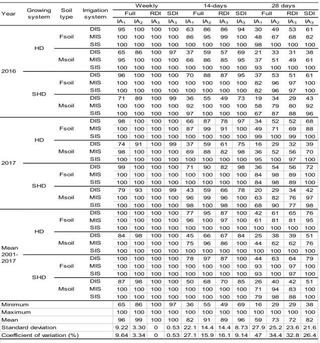
For the weekly interval, with only a few exceptions, IA1, IA2 and IA3 were 100% for
sprinkler system (SIS) and microjet system (MIS) (Table 3). For drip system (DIS), both IA1 and IA2
(referring to full irrigation) were less than 100% in most cases, mainly in Msoils and in the 2016 and 2017 datasets. Under these conditions (HD) groves in Msoils), the 2016 dataset showed the minimum values (IA1 ranging from 65 to 79%,
Table 3). For the same cases, stress was mostly of light type, with IA2 being approximately 90% or
higher (Table 3). This result indicates that the crop was under severe stress for only approximately 10% (=100-IA2) of the irrigation
season. For the deficit strategies, IA3 was always
100% for RDI (any day of extra stress) and was always higher than 97% for SDI (Table 3). For the 14 days interval, the IA indices were still 100% for the SIS cases. Under MIS, the crop experienced a certain degree of stress, mainly in HD groves with full irrigation in Msoil, whereas IA1 sometimes exhibited values below 80%
(Table 3). However, the percentage of days of severe stress generally did not exceed 10% (IA2
90%). In deficit conditions, some values of IA3
were approximately equal to or lower than 90% (Table 3), leading to a certain incidence of extra stress days, mainly for RDI. This interval was sufficient only for olives under full irrigation by DIS for 36-78% of the irrigation season. For Msoils in particular, IA1 was very low, reaching
values below 50% in both HD and SHD groves (Table 3). For the same cases, IA2 values
ranging from 59 to 70% (Table 3) showed a high incidence of severe stress. In deficit conditions, it therefore seems reasonable to apply DIS irrigation with a 14-day interval under only the SDI strategy and in Fsoils (IA3 of 94-100%,
Table 2. Parameters of irrigation for the optimised irrigation scheduling (Over the irrigation season)
Full RDI SDI Full RDI SDI Full RDI SDI Full RDI SDI
DIS 358 227 155 20 13 9 234 148 101 158 142 115 MIS 376 262 183 14 10 7 348 243 170 145 170 140 SIS 431 256 170 5 3 2 752 447 296 136 91 58 DIS 369 241 169 35 24 17 241 157 111 176 168 151 MIS 400 261 183 21 14 10 370 241 169 178 159 141 SIS 466 328 197 7 5 3 812 571 344 173 178 94 DIS 471 320 203 20 14 9 308 209 133 173 182 122 MIS 494 364 241 8 6 4 458 337 223 150 162 113 SIS 525 387 256 8 6 4 915 674 446 150 162 113 DIS 481 317 220 35 24 17 314 207 144 188 177 150 MIS 505 331 251 12 8 6 468 307 232 161 144 136 SIS 550 350 248 11 7 5 959 610 431 165 141 119 DIS 352 249 154 20 14 9 230 163 101 180 153 146 MIS 375 265 157 14 10 6 347 246 146 173 143 121 SIS 428 341 169 5 4 2 746 595 295 152 151 62 DIS 355 263 162 34 25 16 232 172 106 184 178 166 MIS 383 285 164 20 15 9 354 264 152 183 176 138 SIS 395 327 197 6 5 3 689 571 343 138 145 106 DIS 442 324 203 19 14 9 289 212 132 174 156 149 MIS 486 362 241 8 6 4 450 335 223 162 137 137 SIS 516 384 256 8 6 4 899 670 447 162 137 137 DIS 453 339 207 33 25 16 296 222 135 185 180 160 MIS 505 377 249 12 9 6 467 349 231 183 165 164 SIS 504 401 248 10 8 5 878 699 432 158 161 137 DIS 279 191 119 16 11 7 182 125 78 170 138 133 MIS 298 215 131 11 8 5 276 199 121 158 150 125 SIS 342 256 169 4 3 2 595 447 295 127 107 79 DIS 285 201 118 28 20 12 186 132 77 178 161 130 MIS 298 225 127 16 12 7 276 208 117 161 171 116 SIS 329 262 196 5 4 3 574 457 342 130 129 156 DIS 347 250 156 15 11 7 227 163 102 156 138 127 MIS 425 302 181 7 5 3 393 279 167 181 142 97 SIS 452 320 192 7 5 3 787 558 334 181 142 97 DIS 365 268 166 27 20 13 239 175 108 177 172 151 MIS 417 290 204 10 7 5 386 269 189 183 137 153 SIS 448 298 196 9 6 4 780 519 342 184 123 115 279 191 118 4 3 2 182 125 77 127 91 58 550 401 256 35 25 17 959 699 447 188 182 166 414 295 190 15 11 7 471 338 217 166 152 127 74 56 40 9 7 4 244 180 116 17 21 26 18 19 21 62 61 62 52 53 53 10 14 21 Soil type Growing s ys tem Fsoil SHD Fsoil Fsoil Ms oil Fsoil Irrigation s eason length (days) Ms oil Ms oil Total number of irrigation Total energy (kWh/ha) Gross irrigation (mm) Irriga-tion s ys tem Fsoil Ms oil Fsoil Year
Full= full irrigation; RDI= regulated def icit irrigation; SDI= sustained def icit irrigation; HD= high density grove; SHD= super high density grove; Fsoil= fine to medium texture; Msoil= moderately coarse to medium texture; DIS= drip irrigation system; MIS= microjet irrigation system; SIS= sprinkle irrigation system.
Coefficient of variation (%) SHD 2016 HD 2017 HD HD Mean 2001-2017 SHD Ms oil Minimum Maximum Mean Standard deviation Ms oil
For the 28 days interval, only irrigation by SIS in Fsoils resulted in high values (generally >90%) of the IA indices (Table 3). In Msoils, IA1 was
sometimes lower than 90%, mainly for SHD growth. In deficit conditions, IA3 was generally
approximately 100% for SDI and ranged between 88-100% for RDI; the minimum values were associated with SHD groves in Msoils under the RDI strategy (IA3 = 77-88%, Table 3). For both
the microirrigation systems (MIS and DIS), the percentage of stress days was generally higher than 50% (IA1<50% in most cases, Table 3) for
the full irrigation strategy. For DIS in particular, the percentage of severe stress days was also generally higher than 50% (IA2 lower than or
approximately equal to 50%, Table 3). For RDI, the percentage of stress days beyond those scheduled was higher than 50% (IA3<50%) for
DIS and ranged from 3-51% (IA3=97-49%, Table
3) for MIS. With a few exceptions, IA3 was
generally >80% for the SDI strategy applied with MIS; in contrast, IA3 values were always <80%
for DIS.
Overall, the data illustrated above suggest when irrigation is carried out with long intervals (more than a week), the worst conditions in terms of water stress are associated with the full irrigation strategy, Msoils and localised irrigation systems, especially DIS. As expected, this effect depends on the low soil-holding capacity of Msoils and the low percentage of surfaces wetted by the emitters in DIS.
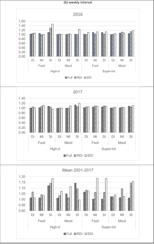
Although the IA and SchE for the 3-day and, under most conditions, weekly intervals were similar to those for OPT management, water and energy consumption should be different. Fig. 2 shows the ratios between Igross applied in 3-day
and weekly intervals and the same variable under OPT scheduling (Igross3-day/IgrossOPT or
Igrossweekly/IgrossOPT). These relationships
assume the same value for the total energy applied in the irrigation season (Ener). Compared to OPT scheduling, water and energy consumption was generally higher under the 3- and weekly interval management schemes (Fig. 2). However, the increases were less than 10% for both the microirrigation systems (DIS and MIS, Fig. 2) but were higher for sprinkling in most cases, mainly for the deficit strategies (RDI and SDI) in the year with the maximum water requirement (2016). In cases involving sprinkling with RDI or SDI in 2016, water and energy consumption could even be 30-48% higher than that under OPT scheduling (Fig. 2).
3.4 Irrigation Management with a Fixed Interval and Quantity
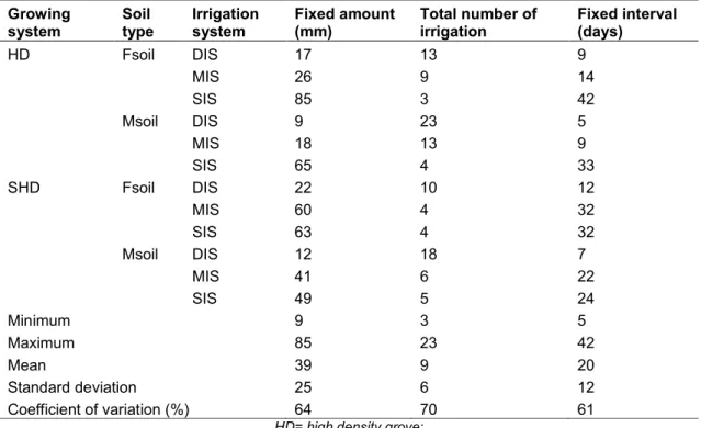
The water quantity and interval were lowest for the HD growing system in Msoil irrigated by DIS (9 mm and 5 days, respectively, Table 4), due to the lower values for RAW and the wetted surface (Table 1). For the opposite reasons, the water quantity and interval were greatest for Msoil and SIS , which showed the highest RAW and a wet surface area of 100%.
For this type of irrigation scheduling, IA was generally very poor (Table 5). Under full irrigation, the crops were stressed for almost the entire irrigation season, mainly under the 2017 meteorological conditions (IA1=2-50%), when the
percentage of severe stress days was also very high (IA2 =63-85%, Table 5). The deficit SDI
strategy and the drip irrigation system (DIS) resulted in the lowest incidence of stress days (IA3 approximately equal or higher than 80%,
Table 5). Intermediate values of IA3 occurred
under the RDI strategy (Table 5).
As expected, the fixed interval, which should be adequate during the initial and final parts of the irrigation season, generally resulted in a lower IA than the optimal value during the central part of the irrigation season, which is the period of
maximum water requirement under the
Mediterranean climate.
SchE was always 100% (any deep loss) under full irrigation and varied from 41 to 100% and 50 to 94% for RDI and SDI, respectively (Table 5). Under full irrigation, the fixed interval indeed always resulted higher than that optimised by the
WB-ET method applied to the three
meteorological datasets used in this study. Under deficit irrigation strategies, deep losses were high under drip systems (DIS) (SchE=41-92%, Table 5) due to the low percentage of wetted area, which did not permit the soil to retain the fixed quantity of irrigation.
3.5 Comparison between the Different Irrigation Scheduling Methods
The irrigation scheduling at variable quantities and intervals (OPT) resulted the most adequate and efficient (no water stress to the plants, no water losses by deep percolation over those due to distribution uniformity) because of the optimisation of both water quantities and intervals determined via the WB-ET method.
For this type of irrigation management, drip systems require less water and energy, allowing considerable savings of approximately 10% and
19%, respectively, of water and 37% and 52%, respectively, of energy compared to microjet and sprinkler systems.
Table 3. Irrigation adequacy (IA1, IA2 and IA3) for irrigation scheduling at variable quantities and weekly, 14-day and 28-day intervals. (IA1 (%) represents the days of the irrigation season without any stress -both light and severe- in fully irrigated plants; IA2 (%) represents the days of the irrigation season without severe stress in fully irrigated plants; IA3 (%) represents the days of the irrigation season without extra stress beyond that specified in the deficit irrigation
strategy RDI or SDI)
RDI SDI RDI SDI RDI SDI IA1 IA2 IA3 IA3 IA1 IA2 IA3 IA3 IA1 IA2 IA3 IA3 DIS 95 100 100 100 63 86 86 94 30 49 53 61 MIS 100 100 100 100 86 95 99 100 48 67 68 82 SIS 100 100 100 100 100 100 100 100 98 100 100 100 DIS 65 86 100 97 37 59 57 69 21 33 31 38 MIS 95 100 100 100 66 86 85 95 37 51 49 61 SIS 100 100 100 100 100 100 100 100 93 100 100 100 DIS 96 100 100 100 70 88 87 95 37 53 51 61 MIS 100 100 100 100 100 100 100 100 82 96 97 100 SIS 100 100 100 100 100 100 100 100 82 96 97 100 DIS 71 89 100 99 36 55 49 73 19 34 29 43 MIS 100 100 100 100 92 100 100 100 58 79 80 92 SIS 100 100 100 100 97 100 100 100 67 87 88 96 DIS 98 100 100 100 66 87 78 97 34 52 52 68 MIS 100 100 100 100 87 99 91 100 49 71 69 88 SIS 100 100 100 100 100 100 100 100 99 100 99 100 DIS 74 91 100 99 37 59 61 75 16 29 32 39 MIS 98 100 100 100 69 88 82 98 36 52 56 70 SIS 100 100 100 100 100 100 100 100 95 100 97 100 DIS 99 100 100 100 71 90 82 98 36 54 56 72 MIS 100 100 100 100 100 100 100 100 84 98 89 100 SIS 100 100 100 100 100 100 100 100 84 98 89 100 DIS 79 93 100 99 43 59 66 78 20 29 34 42 MIS 100 100 100 100 96 99 96 100 63 82 76 97 SIS 100 100 100 100 98 100 98 100 68 90 77 98 DIS 100 100 100 100 77 95 87 100 42 61 65 76 MIS 100 100 100 100 96 100 97 100 61 81 81 95 SIS 100 100 100 100 100 100 100 100 100 100 100 100 DIS 84 98 100 100 45 66 67 84 25 38 39 51 MIS 100 100 100 100 75 96 86 100 44 62 62 76 SIS 100 100 100 100 100 100 100 100 100 100 100 100 DIS 100 100 100 100 78 97 87 100 44 63 64 79 MIS 100 100 100 100 100 100 100 100 93 100 97 100 SIS 100 100 100 100 100 100 100 100 93 100 97 100 DIS 87 98 100 100 50 68 70 85 26 40 42 51 MIS 100 100 100 100 100 100 100 100 71 94 83 100 SIS 100 100 100 100 100 100 100 100 79 98 88 100 65 86 100 97 36 55 49 69 16 29 29 38 100 100 100 100 100 100 100 100 100 100 100 100 96 99 100 100 82 91 89 96 59 73 72 82 9.22 3.30 0 0.53 22.1 14.4 14.4 8.73 27.9 25.2 23.6 21.6 9.64 3.34 0 0.53 27.1 15.9 16.1 9.14 47 34.4 32.8 26.4 28 days Full Full 14-days Fsoil Msoil Soil type Irrigation system Weekly Full Fsoil Msoil Fsoil Msoil SHD Fsoil Msoil HD Msoil SHD Fsoil Msoil Year Growing system Mean 2001-2017 HD 2017 SHD
Full= full irrigation; RDI= regulated deficit irrigation; SDI= s us tained deficit irrigation; HD= high dens ity grove; SHD= s uper high dens ity grove; Fs oil= fine to m edium texture; Ms oil= m oderately coars e to m edium texture; DIS= drip irrigation s ys tem ; MIS= m icrojet irrigation s ys tem ; SIS= s prinkle irrigation s ys tem .Full= full irrigation; RDI= regulated deficit irrigation; SDI= s us tained deficit irrigation; Fs oil= fine to m edium texture; Ms oil=
m oderately coars e to m edium texture; DIS= drip irrigation s ys tem ; MIS= m icrojet irrigation s ys tem ; SIS= s prinkle irrigation s ys tem . 2016 HD Coefficient of variation (%) Minimum Maximum Mean Standard deviation Fsoil
SDI was found to be the lowest consumption irrigation strategy in terms of both water and energy. SDI permitted average savings of approximately 36% and 54% for water and energy compared to RDI and full irrigation, respectively. Compared to HD orchards, SHD
orchards required approximately 32% more water and energy on average. In reference to the mean meteorological conditions, HD orchards (approximately 280 plants/ha) drip irrigated under the SDI strategy showed minimum water and energy requirements of approximately 120 mm
Fig. 2. Gross irrigation used for management with variable amounts and fixed intervals relative to optimised scheduling. (a) 3 day interval; (b) 7 day interval (DI= drip irrigation system; MI= microjet irrigation system; SI= sprinkle irrigation system; Fsoil= fine to medium texture; Msoil=
moderately coarse to medium texture; High-d= high-density grove; Super-hd= super-high-density grove; Full= full irrigation; RDI= regulated deficit irrigation; SDI= sustained deficit
irrigation) (b) weekly interval 0.00 0.20 0.40 0.60 0.80 1.00 1.20 1.40 1.60 DI MI SI DI MI SI DI MI SI DI MI SI
Fsoil Msoil Fsoil Msoil
High-d Super-hd
2016
Full RDI SDI
0.00 0.20 0.40 0.60 0.80 1.00 1.20 1.40 DI MI SI DI MI SI DI MI SI DI MI SI
Fsoil Msoil Fsoil Msoil
High-d Super-hd
2017
Full RDI SDI
0.90 0.95 1.00 1.05 1.10 1.15 1.20 DI MI SI DI MI SI DI MI SI DI MI SI
Fsoil Msoil Fsoil Msoil
High-d Super-hd
Mean 2001-2017
Table 4. Irrigation parameters for irrigation scheduling at a fixed quantity and interval Growing system Soil type Irrigation system Fixed amount (mm) Total number of irrigation Fixed interval (days) HD Fsoil DIS 17 13 9 MIS 26 9 14 SIS 85 3 42 Msoil DIS 9 23 5 MIS 18 13 9 SIS 65 4 33 SHD Fsoil DIS 22 10 12 MIS 60 4 32 SIS 63 4 32 Msoil DIS 12 18 7 MIS 41 6 22 SIS 49 5 24 Minimum 9 3 5 Maximum 85 23 42 Mean 39 9 20 Standard deviation 25 6 12 Coefficient of variation (%) 64 70 61
HD= high density grove; SHD= super high-density grove;
Fsoil= fine to medium texture; Msoil= moderately coarse to medium texture;
DIS= drip irrigation system; MIS= microjet irrigation system;
SIS= sprinkle irrigation system
and 80 KWh/ha, respectively. In contrast, SHD orchards (approximately 1700 plants/ha) fully irrigated by DIS showed higher water and energy requirements (approximately 350 mm and 230 KWh/ha, respectively). A typical HD olive orchard drip irrigated under the RDI strategy required approximately 200 mm of water and 180 KWh/ha of energy. The irrigation requirements are of the same order of magnitude as those suggested in Andalucia, Spain [4].
Under irrigation scheduling with variable quantities and fixed intervals, the 3 days interval ensured performance similar to the OPT scheduling in terms of efficiency, but with a slight increase (less than 10%) in water and energy requirements. The weekly interval resulted in high scheduling efficiency (SchE), but with light water stress for HD groves in Msoils fully irrigated by drip systems. Due to the high percentage of stress days (both light and severe), drip and microjet irrigation were not feasible for 14- and 28-day intervals under most of the conditions examined. With a 14 days
interval, microjet systems were acceptable under only the SDI strategy. Sprinkler systems resulted in a low percentage of stress days and a high SchE, but water and energy requirements were up to 40% higher than those with OPT scheduling.
For all the conditions examined, irrigation scheduling with a fixed quantity and interval resulted in a high percentage of stress days. Furthermore, water losses due to deep percolation were high for both the RDI and SDI strategies.
It should be noted that early water deficit was detected in all the three meteorological periods analysed (2016, 2017 and mean 2001-2017). In fact, the date of the first irrigation event varied from April 22nd to May 2nd for both full and RDI irrigation and from May 14th to May 29th for SDI, in contrast with the traditional irrigation scheduling according to farmers, in the area examined, irrigate olive orchards from mid-June to September.
Table 5. Irrigation adequacy (IA1, IA2 and IA3) and irrigation scheduling efficiency for irrigation management at a fixed quantity and interval (IA1 (%) represents the days of the irrigation season without any stress -both light and severe- in fully irrigated plants; IA2 (%) represents
the days of the irrigation season without severe stress in fully irrigated plants; IA3 (%) represents the days of the irrigation season without extra stress beyond that specified in the
deficit irrigation strategy RDI or SDI).
RDI SDI IA1 IA2 IA3 IA3 DIs 14 27 70 85 100 89 70 MIs 15 29 79 96 100 89 75 SIs 28 64 79 96 100 89 82 DIs 12 23 60 68 100 61 70 MIs 12 26 73 79 100 61 69 SIs 12 48 75 88 100 71 78 DIs 8 23 64 75 100 78 89 MIs 13 31 70 87 100 83 93 SIs 13 31 70 87 100 83 93 DIs 5 16 47 48 100 78 90 MIs 10 23 67 77 100 85 94 SIs 12 24 68 79 100 80 90 DIs 2 20 56 85 100 72 59 MIs 3 30 48 76 100 78 64 SIs 50 83 55 77 100 92 67 DIs 1 8 41 66 100 41 57 MIs 7 34 55 78 100 55 58 SIs 7 34 66 82 100 66 68 DIs 2 9 39 76 100 92 74 MIs 7 34 58 81 100 95 80 SIs 7 34 63 81 100 100 80 DIs 1 4 23 63 100 93 74 MIs 4 13 48 76 100 98 80 SIs 5 17 55 77 100 93 77 DIs 51 85 76 97 95 61 52 MIs 53 87 77 97 100 67 57 SIs 73 88 78 97 100 77 68 DIs 31 58 60 75 95 61 50 MIs 52 81 73 87 94 61 51 SIs 68 83 75 87 100 71 62 DIs 4 19 64 86 100 78 65 MIs 27 74 70 86 100 83 72 SIs 27 74 70 86 100 83 72 DIs 2 10 47 48 100 78 90 MIs 9 36 67 77 100 85 94 SIs 15 57 68 79 100 80 90 1 4 23 48 94 41 50 73 88 79 97 100 100 94 18 40 63 80 100 78 74 20 26 13 11 1 14 13 107 66 21 14 1 17 18 Minimum Standard deviation Coefficient of variation (%) Mean 2001-2017 HD Maximum Mean Fsoil Msoil SHD Fsoil Msoil SHD Year Gro-wing system 2016 HD Fsoil Msoil SHD Fsoil Msoil
Full= full irrigation; RDI= regulated deficit irrigation; SDI= sustained def icit irrigation; HD= high density grove; SHD= super high density grove; Fsoil= fine to medium texture; Msoil= moderately coarse to medium texture; DIS= drip irrigation system; MIS= microjet irrigation system; SIS= sprinkle irrigation system.
Fsoil Msoil Soil type Fsoil Msoil
Full RDI SDI
Scheduling efficiency (%) Irrigation adequacy (%) Full Irrigation system 2017 HD
4. CONCLUSION
The main results of the research showed that the traditional irrigation strategy at fixed quantity and interval is not adequate to achieve high efficiency in the irrigation of olive orchards, from both the agronomic (reduction of crop water stress) and economic (reduction of water and energy requirements) point of view.
The optimisation of the irrigation scheduling requires the estimate of the water quantity to deliver in each irrigation in both the irrigation management at variable and fixed interval. The evapotranspiration-water balance model is an efficient and (relatively) simple tool to foresee the quantities and the dates of irrigation during the irrigation season.
The adoption of a fixed interval, which is preferred by the farmers for practical reasons, is feasible after verifying that it is adequate for the type of soil, plant density and irrigation system used. In the case of drip systems, it is not advisable to adopt intervals longer than one week. A means of lengthening the interval would be to increase the wetted area through the installation of more than two laterals per row, but this strategy is not feasible for practical and economic reasons as it can make irrigation costs prohibitive for a crop such as olive, in which large gains are not possible. When water agencies supply water at intervals longer than a week, the farmers should build storage facilities.
The irrigation season length should be longer respect the traditional one. Early water deficit (at the end of April or in the first decade of May) were detected in all the meteorological periods studied. Similarly, the results of the simulation showed that the irrigation season ends in October, mainly when localised irrigation systems were used. In contrast, with the traditional irrigation scheduling, farmers, in the area examined, irrigate olive orchards from mid-June to September.
Overall, in the area examined or in similar climatic conditions, considering also the risks to development of diseases such as Verticillium, drip irrigation systems and a weekly interval are advisable for olive groves, as highlighted by Gucci and Fereres [3].
From the methodological point of view, the
simulated cases can be considered
representative of both the real and potential
conditions experienced by olive grown in the Southern Italy environment.
ACKNOWLEDGEMENTS
This work was funded by the Italian Ministry of Education, University and Research (MIUR) through the PON Ricerca e competitività 2007– 2013 (PON03PE_00090_02).
COMPETING INTERESTS
Authors have declared that no competing interests exist.
REFERENCES
1. Carr MKV. The water relations and irrigation requirements of olive (Olea europaea L.): A review. Experimental Agriculture. 2013;49(4):597-639.
Available:https://dx.doi.org/10.1017/S0014 479713000276
2. Fernández JE. Understanding olive adaptation to abiotic stresses as a tool to increase crop performance. Environ. Exp. Bot. 2014;10:158–179.
Available:https://dx.doi.org/10.1016/j.envex pbot.2013.12.003
3. Gucci R, Fereres E. Fruit trees and vines. Olive. In crop yield response to water. FAO Irrigation and drainage paper. 2012;66: 300-313.
(Accessed 15 February 2018)
Available:http://www.fao.org/docrep/016/i2 800e/i2800e.pdf
4. Instituto de Investigatión y Formación Agraria y Pesquera Junta de Andalucia. Produción Integrada de Olivar; 2011. (Accessed 20 January 2018)
Available:http://www.juntadeandalucia.es/e xport/drupaljda/1337159656Produccixn_Int egrada_Olivar.pdf
5. Torres M, Pierantozzi P, Searles P, Rousseaux MC, García-Inza G, Miserere A, Bodoira R, Contreras C, Maestri D. Olive cultivation in the southern hemisphere: Flowering, water require-ments and oil quality responses to new crop environments. Front Plant Sci. 2017; 8:1830.
Available:http://dx.doi.org/10.3389/fpls.201 7.01830
6. Iniesta F, Testi L, Orgaz F, Villalobos FJ. The effects of regulated and continuous deficit irrigation on the water use, growth and yield of olive trees. Europ. J. Agronomy. 2009;30:258-265.
Available:http://dx.doi.org/10.1016/j.eja.20 08.12.004
7. Fereres E, Goldhamer DA, Parsons LR. Irrigation water management of horti-cultural crops. Hortscience. 2003;38(5): 1036-1042.
8. Capra A, Scicolone B. Simulation-based evaluation of the efficiency of different irrigation scheduling strategies. Proceedings of XXX CIOSTA-CIGR V Congress, Torino. 2003;1238-1246. 9. Capra A, Scicolone B. Progettazione e
gestione degli impianti di irrigazione, seconda edizione. Bologna: Edagricole; 2016. Italian.
10. Keller J, Bliesner RD. Sprinkle and trickle irrigation. New York: AVI Book; 1990. 11. Lamm FR, Ayars JE, Nakayama FS.
Microirrigation for crop production. Amsterdam: Elsevier; 2007.
12. English MJ. Deficit irrigation: An analytical framework. J. of Irr. and Drain. Eng. ASCE. 1990;116(3):399-412.
13. Capra A, Consoli S, Scicolone B. Deficit irrigation: Theory and practice. In: Alonso D, Iglesias HJ, editors. Agricultural Irrigation Research Progress. Hauppauge Ny: Nova Science Pub.; 2008.
14. Fereres E, Soriano MA. Deficit irrigation for reducing agricultural water use. J Exp Bot. 2007;58(2):147-159.
15. Agüero Alcaras LM, Rousseaux MC, Searles PS. Responses of several soil and plant indicators to post-harvest regulated deficit irrigation in olive trees and their potential for irrigation scheduling. Agri-cultural Water Management. 2016;171:10-20.
16. Girón IF, Corell M, Martín-Palomo MJ, Galindo A, Torrecillas A, Moreno F, Moriana A. Feasibility of trunk diameter fluctuations in the scheduling of regulated deficit irrigation for Table olive trees without reference trees. Agricultural Water Management. 2015;161:114-126.
17. García-Tejera O, López-Bernal Á, Orgaz F, Testi L, Villalobos FJ. Analysing the combined effect of wetted area and irrigation volume on olive tree transpiration using a SPAC model with a multi-com-partment soil solution. Irrigation Science. 2017;35:409–423.
DOI: 10.1007/s00271-017-0549-5
18. Mesa-Jurado MA, Berbel J, Orgaz F. Estimating marginal value of water for irrigated olive grove with the production function method. Spanish Journal of
Agricultural Research. 2010;8(S2):S197-S206.
(Accessed 25 January 2018) Available:www.inia.es/sjar
19. Egea G, Fernández JE, Alcon F. Financial assessment of adopting irrigation technology for plant-based regulated deficit irrigation scheduling in super HIGH-Density olive orchards. Agricultural Water Management. 2017;187:47-56.
20. Gómez-Rico A, Salvador MD, Moriana A, Pérez D, Olmedilla N, Ribas F, Fregapane G. Influence of different irrigation strategies in a traditional Cornicabra cv olive orchard on virgin olive oil composition and quality. Food Chem. 2007;100:568-578.
21. Motilva MJ, Tovar MJ, Romero MP, Alegre S, Girona J. Influence of regulated deficit irrigation strategies applied to olive trees (Arbequina cultivar) on oil yield and oil composition during the fruit ripening period. J. Sci. Food Agric. 2000;80:2037-2043.
22. Servili M, Esposto S, Lodolini E, Selvaggini R, Taticchi A, Urbani S, Montedoro G, Serravalle M, Gucci R. Irrigation effects on quality, phenolic composition, and selected volatiles of Virgin olive oils Cv. Leccino. J. Agric. Food Chem. 2007;55(16):6609-6618.
(Accessed 20 April 2018)
Available:https://pubs.acs.org/doi/pdfplus/1 0.1021/jf070599n
23. Capra A, Scicolone B. Water quality and distribution uniformity in drip/trickle irrigation systems. J. Agricultural Engine-ering Research. 1998;70:355-365.
24. Smith M, Pereira LS, Beregena J, Itier J, Goussard B, Ragab R, Tollefson L, Van Hoffwegen P. Irrigation scheduling: From theory to practice. Rome: FAO Water Report 8, ICID & FAO; 1996.
25. Howell TA, Meron M. Irrigation scheduling. In Lamm FR, Ayars JE, Nakayama FS editors. Microirrigation for crop production. Amsterdam: Elsevier; 2007.
26. Lamm FR, Rogers DH. The importance of irrigation scheduling for marginal capacity systems growing corn. Applied Engine-ering in Agriculture. 2015;31(2):261-265. Available:http://dx.doi.org/10.13031/aea.31 .10966
27. Fereres E, Evans RG. Irrigation of fruit trees and vines: An introduction. Irrigation Science. 2006;24:55-57.
28. Heerman DF. Irrigation scheduling. In Pereira LS, Fedder RA, Gilley RA, Lesaffre
B, editors. Sustainability of irrigated agri-culture. Dordrecht: Kluwer Academic Publishers; 1996.
29. Gu Z, Qi Z, Mac L, Gui D, Xu J, Fang Q, Yuan S, Feng G. Development of an irrigation scheduling software based on model predicted crop water stress. Com-puters and Electronics in Agriculture. 2017;143:208-221.
30. Pereira LS, Oweis T, Zairi A. Irrigation management under water scarcity. Agri-cultural Water Management. 2002;57:175-206.
31. Maheshwari BL, Plunkett M. Best practice irrigation management and extension in peri-urban landscapes – Experiences and insights from the Hawkesbury–Nepean catchment, Australia. Journal of Agri-cultural Education and Extension. 2015; 21(3):267-282.
32. Stirzaker RJ. When to turn the water off: Scheduling micro-irrigation with a wetting front detector. Irrigation Science. 2003;22: 177-185.
33. Pérez-Rodríguez M, Alcántara E, Amaro M. The influence of irrigation frequency on the onset and development of Verticillium wilt of olive. Plant disease. 2015;99(4):488-495.
Available:https://doi.org/10.1094/PDIS-06-14-0599-RE
34. Pérez-Rodríguez M, Orgaz I, López-Escudero FJ. Effect of the irrigation dose on Verticillium wilt of olive. Scientia Horticulturae. 2015;197:564-567.
35. Navas-Cortés JA, Landa BB, Mercado-Blanco J, Trapero-Casas JL, Rodríguez-Jurado D, Jiménez-Díaz RM. Spatiote-mporal analysis of spread of infections by Verticillium dahliae pathotypes within a high tree density olive orchard in Southern Spain. Ecology and Epidemiology. 2008; 98(2):167-180.
36. Italian National Institute of Statistics (ISTAT); 2017.
(Accessed 12 December 2017) Available:http://agri.istat.it
37. Fereres E, Villalobos FJ, Orgaz F, Testi L. Water requirements and irrigation scheduling in olive. Acta Horticulturae. 2011;888:31-39.
38. Allen RG, Pereira LS, Raes D, Smith M. Crop evapotranspiration. Guidelines for computing crop water requirements. Rome: FAO Irrigation and Drainage Paper 56; 1998.
39. Acutis M, Donatell M. SOILPAR 2.00: software to estimate soil hydrological parameters and functions. Europ J Agronomy. 2003;18(3-4): 373-377.
40. Agenzia Regionale per lo Sviluppo della Calabria (ARSSA). I suoli della Calabria. Carta dei suoli della Regione Calabria; 2003. Italian.
41. CORINE land cover. (Accessed April 2015)
Available:http://www.eea.europa.eu/data- and-maps/data/corine-land-cover-2006-clc2006-100-m-version-12-2009
42. Burt CM, Clemmens AJ, Strelkoff KH. Irrigation performance measurements: efficiency and uniformity. Journal of Irrigation and Drainage Engineering. 1997; 123(6):423–442.
43. Davis SL, Dukes MD. Irrigation scheduling performance by evapotranspiration based controllers. Agricultural Water Manage-ment. 2010;98:19–28.
Available:http://dx.doi.org/10.1016/j. agwat.2010.07.006
44. McCready MS, Dukes MD. Landscape irrigation scheduling efficiency and adequacy by various control technologies. Agricultural Water Management. 2011;98: 697–704.
Available:http://dx.doi.org/10.1016/j.agwat. 2010.11.007
45. Capra A, Consoli S, Scicolone B. Long-term climatic variability in Calabria and effects on drought and agrometeorological parameters. Water Resources Manage-ment. 2013;27(2):601-617.
DOI: 10.1007/s11269-012-0204-0
_________________________________________________________________________________ © 2018 Capra and Scicolone; This is an Open Access article distributed under the terms of the Creative Commons Attribution License (http://creativecommons.org/licenses/by/4.0), which permits unrestricted use, distribution, and reproduction in any medium, provided the original work is properly cited.
Peer-review history:
The peer review history for this paper can be accessed here: http://www.sciencedomain.org/review-history/27281