DOCTORAL SCHOOL UNIVERSITA’ MEDITERRANEA DI REGGIO CALABRIA DIPARTIMENTO DI INGEGNERIA DELL’INFORMAZIONE, DELLE INFRASTRUTTURE E DELL’ENERGIA SOSTENIBILE (DIIES) PHD IN INFORMATION ENGINEERING
S.S.D. ING-INF/02 XXXII CICLO
NUMERICAL MODELING AND REALIZATION
OF MICROWAVE DEVICES FOR
DIELECTRIC AND METALLIC ACCELERATORS
CANDIDATE
Giorgio Sebastiano MAURO
ADVISORS
Dott. Ing. Luigi CELONA
Prof. Gino SORBELLO
COORDINATOR
P
rof. Tommaso
I
SERNIA
Finito di stampare nel mese di Febbraio 2020
Edizione Quaderno N. 46
Collana Quaderni del Dottorato di Ricerca in Ingegneria dell’Informazione Curatore Prof. Claudio De Capua
ISBN 978-88-99352-39-4
Università degli Studi Mediterranea di Reggio Calabria Salita Melissari, Feo di Vito, Reggio Calabria
G
IORGIO
S
EBASTIANO
M
AURO
NUMERICAL MODELING AND REALIZATION
OF MICROWAVE DEVICES FOR
DIELECTRIC AND METALLIC ACCELERATORS
The Teaching Staff of the PhD course in
INFORMATION ENGINEERING
consists of: Claudio DE CAPUA (coordinator)
Antonio IERA Antonella MOLINARO Giuseppe RUGGERI Giuseppe ARANITI Francesco Giuseppe DELLA CORTE Riccardo CAROTENUTO Fortunato PEZZIMENTI Tommaso ISERNIA Giovanni ANGIULLI Francesco Antonio BUCCAFURRI Domenico URSINO Gianluca LAX Rosario CARBONE Sofia GIUFFRE’ Salvatore COCO Domenico ROSACI Valerio SCORDAMAGLIA Andrea Francesco MORABITO Pasquale Giuseppe Fabio FILIANOTI Aimè LAY EKUAKILLE Sandro RAO Giacomo Domenico Savio MESSINA Mariateresa RUSSO Pier Luigi ANTONUCCI Patrizia FRONTERA Mariantonia COTRONEI Giuliana FAGGIO Claudia CAMPOLO Voicu GROZA Antoine O. BERTHET Dominique DALLET Luigi Giuseppe CELONA Lorenzo CROCCO Rosario MORELLO Ivo RENDINA
Abstract
This thesis deals about analytical, numerical and experimental procedures for the design and realization of metallic and dielectric particle accelerators, along with related devices.
The first part, performed in the European Spallation Source (ESS) framework, is dedicated to the metallic accelerators and in particular to the ESS Drift Tube Linac. The numerical simulation of such structures, large cylindrical cavities com-posed of many cells, is not an easy task but results an essential step in the cavity electromagnetic design. In order to ease the simulation of large metallic structures such as the DTL, some analytical and numerical methods have been developed. These methods are able to predict, the frequency error introduced when the real structure is discretized inside the commercial electromagnetic simulators or can cre-ate computationally advantageous symmetries into the considered structure. These techniques have been employed in the electromagnetic design of a DTL tank cold model, which has been realized in order to test the field measurement setup and to obtain a field stabilization procedure to counteract random manufacturing errors that could degrade the accelerator performances.
The second part of this thesis, performed in the DiElectric and METallic Ra-diofrequency Accelerator (DEMETRA) framework, is focused on the study and nu-merical simulation of Dielectric Laser Accelerator devices. In particular, the woodpile structure has been studied through the use of numerical tools and an alumina pro-totype, operating at X-band, has been realized and experimentally characterized in terms of S-parameters and on-axis electric field, showing very good agreement with the numerical results. The knowledge acquired with the alumina prototype has led the way to the realization of a silicon prototype, operating in the W-band, which has been successfully characterized.
Contents
1 Introduction . . . 1
1.1 Linear accelerators . . . 2
1.2 Proton LINACs VS electron LINACs . . . 3
1.2.1 European Spallation Source (ESS) LINAC . . . 8
1.2.2 Dielectric Laser Accelerators (DLA) and high gradient electron sources . . . 9
1.3 Particle Acceleration in RF fields . . . 11
1.3.1 Figures of merit of a linear accelerator . . . 12
Part I Metallic accelerating structures 2 Numerical study of metallic accelerators . . . 21
2.1 Problem definition . . . 21
2.1.1 Symmetry and 2D reduced models . . . 22
2.1.2 Curved surfaces and mesh . . . 23
2.2 Proposed approach . . . 24
2.2.1 2D reference simulation . . . 25
2.2.2 3D curved boundaries and mesh error prediction . . . 26
2.3 Numerical validation . . . 28
2.3.1 Mesh error prediction formula application . . . 28
2.3.2 Equivalent volume method . . . 29
2.4 Final considerations . . . 32
3 Fabrication, assembly and experimental validation of ESS DTL tank 2 cold model . . . 33
3.1 Cold model assembly and alignment . . . 34
3.2 Bead pull measurement technique . . . 35
II Contents
3.2.2 Perturbator radius estimation . . . 39
3.2.3 Bead pull setup for tank 2 cold model . . . 41
3.3 Data analysis and post processing . . . 42
3.3.1 Phase drift correction . . . 42
3.3.2 Accelerating field evaluation: integral method vs peak field method . . . 44
3.3.3 Tilt sensitivity . . . 45
Local tilt sensitivity . . . 46
3.4 Post-coupler stabilization . . . 47
3.4.1 Resonant coupling . . . 49
3.4.2 Stabilization procedure . . . 54
3.4.3 Cavity confluence . . . 54
3.4.4 Post-coupler resonance lengths . . . 57
3.4.5 Post-coupler stabilization lengths . . . 59
4 X-Band Mode Launcher . . . 65
4.1 The Steele non-resonant perturbation theory . . . 66
4.2 Cold model prototype . . . 68
4.2.1 S-parameters measurement . . . 69
4.2.2 Electric field measurement . . . 71
Part II Towards a Dielectric Laser Accelerator 5 Introduction . . . 79
6 2D PhC coupler . . . 81
7 Electromagnetic Band Gap (EBG) structures . . . 85
8 Numerical study of an EBG device: the woodpile structure . . . 89
8.1 3D full wave simulations . . . 92
8.1.1 Optimization of the launch metallic waveguides . . . 93
8.1.2 Study of the lateral dimension of the crystal . . . 94
9 Experimental results . . . 99
9.1 Fabrication of the 18 GHz woodpile waveguide . . . 99
9.2 S-parameters measurement . . . 100
9.3 Electric field measurement along the z channel . . . 102
Contents III
10 W-band woodpile waveguide . . . 107
10.1 Realization and experimental validation . . . 109
11 Conclusions and perspectives . . . 113
12 Acknowledgments . . . 117
Bibliography . . . 119
List of Figures
1.1 Schematic of a particle bunch accelerated by an electric field. . . 3 1.2 Drift Tube Linac model. . . 3 1.3 Typical accelerating field of a metallic linear accelerator. Drift tubes
are placed in the zones where a decelerating field would be otherwise present, creating a field-free region for travelling particles. . . 5 1.4 Schematic of a DTL. The structure can be divided into cells, extending
from the center of one drift tube to the center of the next. The cell length for a structure operating in the 0-mode (i.e. the distance from two drift-tube centers) is βλ, with β increasing as the particle travels along the structure. The drift-tubes are attached to the cavity outer wall through metal cylinders called ’stems’. . . 5 1.5 Relativistic particle velocity (protons and electrons) as function of
gained kinetic energy. . . 7 1.6 Schematic of a typical travelling wave structure for particle acceleration. 7 1.7 Schematic of the ESS accelerating system. . . 9 1.8 Drift Tube Linac HFSS simulation: the meshing elements
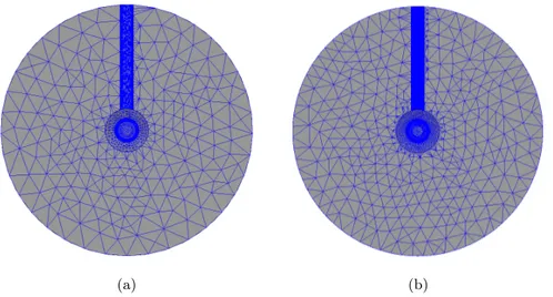
(tethraedrons) used for the cavity representation are visible. . . 10 1.9 Early (E), stable (S), late (L) and unstable (U) particle phases. . . 11 1.10 Accelerating gap of length g. The field inside the gap is also shown. . . . 12 2.1 3D representation of a Drift Tube Linac cavity cell: (a) full structure
and (b) slice. . . 23 2.2 (a) Front view of a simulated circular cavity. Highlighted in red is the
difference between real and simulated profile. (b) Circular sector of a cylindrical cavity. . . 24
VI List of Figures 2.3 Rotational symmetry and stem: (a) 3D and (b) side view of a DTL
cell model. Central element is called drift tube and is attached to the cavity outer wall through a metal cylinder called stem. The presence of stem breaks axial rotation symmetry and this makes necessary full 3D simulations. . . 25 2.4 (a) Superfish DTL cell representation. Thanks to the rotational
symmetry, only half of the structure is actually simulated by using an extremely fine mesh. (b) Electric field Ez obtained for the considered
cell. . . 26 2.5 (a) HFSS cell front face mesh using α = 10◦. (b) HFSS cell front face
mesh using α = 5◦. . . . 30
2.6 Application of the equivalent volume method to half DTL cell in HFSS. A normal deviation angle of α = 5◦ is also used to ensure
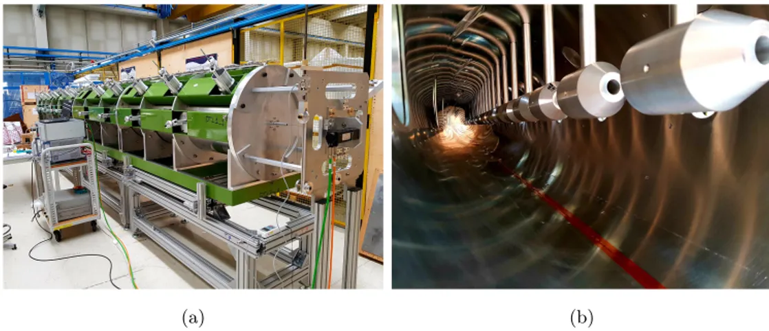
accurate results. . . 31 3.1 ESS DTL tank 2 cold model: (a) assembled model comprehensive of
post-couplers and tuners; (b) internal view of the cavity with mounted drift tubes. . . 34 3.2 DTL tank 2 assembly steps: (a) drift tubes and modules alignment;
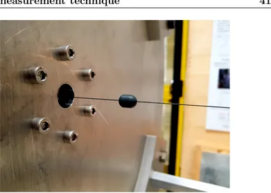
(b) the used laser tracker with its control laptop. . . 35 3.3 Typical bead-pull setup for field measurement: a small dielectric or
metallic bead, attached to a thin dielectric wire, is pulled through a cavity while the electric and/or magnetic field measure versus position is performed. . . 37 3.4 Bead pull measure ( |S21| vs bead position) of the operation mode
TM010 in a DTL cavity. . . 39
3.5 (a) Drift Tube Linac cell and (b) parameters (Superfish simulation). . . 40 3.6 Example of Teflon bead used for bead-pull measures on the ESS DTL
tank 2 cold model. . . 41 3.7 Setup used for bead pull measurements. VNA and motor are controlled
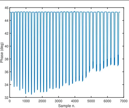
through a LabView script that acquires and saves the measures. . . 41 3.8 Phase shift correction: (a) original acquired measure, (b) measure
with phase correction applied. . . 43 3.9 Comparison of average axial field of DTL tank 2 cold model: direct
integration (red curve) VS peak field method (blue curve). . . 45 3.10 Tilt-sensitivity curve for a particular configuration. For the i-th cell,
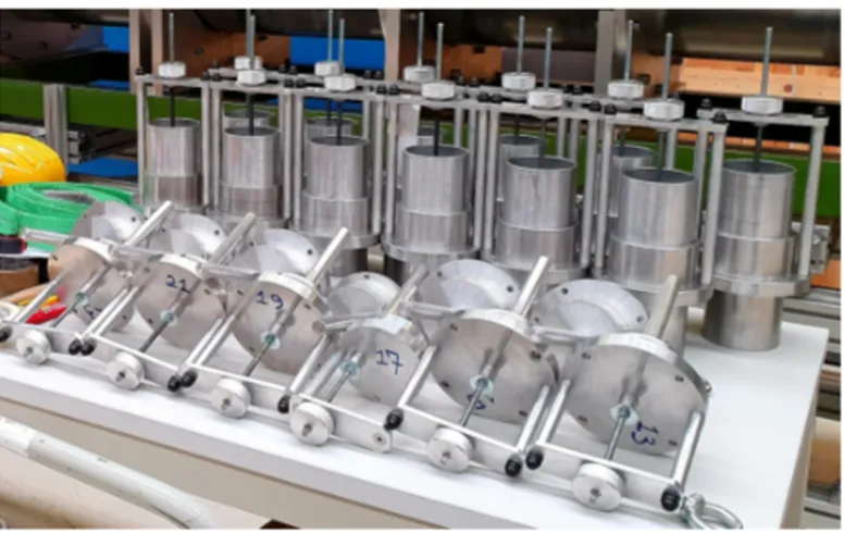
List of Figures VII 3.11 Post-couplers (lower photo side) and tuners (upper photo side) used
for the RF tuning of the ESS DTL tank 2 cold model. . . 47 3.12 Post-coupler arrangement for ESS DTL tank 2 simulated model:
in the image, the low energy side of the tank is on the left, while the high energy side is on the right. The front view is visible in the inset: vertical bars are the stems while the horizontal bars are the
post-couplers used for the field stabilization. . . 48 3.13 Post-couplers with lpc= 190 mm: perturbed fields and tilt-sensitivity. . 49
3.14 Field distribution of the (a) 0-mode, (b) π/2-mode and (c) π-mode for a seven-cell cavity. . . 50 3.15 Dispersion diagram (frequency vs. phase) of a system composed by
seven oscillators. . . 51 3.16 Dispersion curve of a system composed by two set of oscillators. If the
resonating frequencies of the two sets of oscillators do not match, a
stop band opens in the curve. . . 52 3.17 Sketch of a Coupled Cavity Linac (CCL). Accelerating and side
coupling cells are visible. . . 53 3.18 Photo of the VNA screen: cavity 0-mode (TM010) is marked with M1,
cavity 1-mode (TM011) is marked with M3 while post-coupler 1-mode
(PC1) is marked with M2. The cavity reaches the confluence point
when all the s are inserted of 175.2 mm. . . 56 3.19 Phase measures of the post-coupler 1-mode (a), cavity 1-mode (b) and
cavity 0-mode (c). The confluence can be observed from the symmetry of the first two modes. . . 56 3.20 (a) TM010 resonance frequency vs. insertion length plot for the 2-nd
post-coupler of the DTL tank 2. The resonance length is found around 147 mm. (b) T S2′ vs. insertion length plot for the 2-nd post-coupler
of the DTL tank 2. The curve has a pole around 147 mm, where it
changes sign, and reaches 0 value around a length of 164 mm. . . 57 3.21 Resonance frequency vs. length and equivalent T Sn′ vs. length curves
for post-couplers 4, 12, 16, 20, 22. . . 58 3.22 Tilt sensitivity curve relative to the post-coupler configuration with
equal penetration length of lconf luence= 175.2 mm. . . 60
3.23 Results obtained at the end of the stabilization campaign. . . 61 3.24 Results of the stabilization campaign with odd post-couplers length
VIII List of Figures 4.1 HFSS 3D model of the X-band mode launcher structure. . . 66 4.2 Schematic of a device in which the field have to be measured. It
has just one waveguide (or transmission line) port through which electromagnetic energy is permitted to pass into its interior. It can
have any size or shape. . . 67 4.3 Manufactured aluminium mode launchers for cold tests: (a) inside
of the single mode launcher, (b) two mode launchers with mounted
cover, (c) mode launcher assembled in back-to-back-configuration. . . 69 4.4 Simulated (red curves) vs. measured (blue curves) S-parameters for
the full devices in back-to-back configuration: |S11| on the left column,
|S12| on the right column. A very good agreement between the two is
visible, despite some numerical simulation spikes. . . 70 4.5 (a) Bead-pull setup used for the field (∆|S11|) measurements on
the mode launcher. (b) Circular flange used for the azimuthal field
measurements. . . 72 4.6 Measured ∆|S11| values vs. bead position (blue curves) and
comparison with HFSS electric field simulations (red curves). (a) The |S11| values have been taken along the circular waveguide axis,
on an interval of 100 mm starting from the cut-off flange, for the axial measurement. (b) The |S11| values have been taken along a
circumference of radius r = 4 mm at the axial position z ≃ 90 mm for the azimuthal measurement. . . 73 6.1 3D model of the simulated 2D directional coupler based on the
triangular lattice. The telecom waveguide, named WG2, possesses a TE10 mode that, after a beating period, transfer itself into the
accelerating waveguide, named WG1, becoming a TM-like mode that have a predominant field component along the waveguide axis and is thus suitable for particle acceleration. . . 82 6.2 3D and front view of a PhC coupler based on the woodpile crystal.
Two defects has been practiced on the dielectric structure: on the left is placed the telecom waveguide and on the right is placed the
accelerating waveguide. . . 83 7.1 One-, two- and three-dimensional photonic crystals, having periodicity
along one or more axes. Different colors in each crystal represents
List of Figures IX 7.2 The FCC lattice. . . 86 8.1 The woodpile structure: it is composed of layers of bricks (or rods)
stacked together with alternating orthogonal orientation. . . 89 8.2 Simple tetragonal lattice. The first Brillouin zone is the path
highlighted in red. . . 90 8.3 (a) Woodpile structure primitive cell with its geometrical parameters:
brick width w, height h, and lattice period d. The structure repeats itself every four layers, along y direction. (b) Calculated band structure. The complete photonic band-gap reaches a maximum value of 15.2% when w = 1.9 mm and h = 2.38 mm. . . 91 8.4 Woodpile waveguide front view: the structure has been made
symmetric in the vertical direction (xz symmetry plane) for better mode confinement. A rectangular wd× hd defect has been practiced
in the structure center in order to confine a guided mode. . . 92 8.5 Projected band diagrams for the designed structure. By imposing
d = 6.73 mm the dispersion curve (in red) of a guided mode intersects the frequency of interest (black horizontal line). The other two blue curves visible inside the band-gap are the dispersion curves of two additional modes supported by the hollow core EBG structure. However, they are not coupled in the presented setup due to the different polarization, propagation constant and symmetry with
respect to the exciting TE10 mode. . . 92 8.6 3D model of the woodpile device. In order to feed the structure, two
standard WR62 metallic waveguides (grey components) are adopted. Plexiglass lateral enclosure (light blue components) is also visible. . . 93 8.7 (a) Transverse mode profile ewg of the WR62 waveguide (standard
height bW R62 = 7.8994 mm. (b) Mode profile of the woodpile
waveguide (z = 0 mm cut): ewp vector field superimposed to the
field color-map showing that both the obtained polarization and field distribution resemble the ewg of the feeding WR62 waveguide. (c)
Mode profile of the woodpile waveguide (z = d/2 cut): ewpvector field
superimposed to color-map. . . 95 8.8 Woodpile waveguide S-parameters, standard WR62 waveguides (red
curves) vs. custom metallic waveguides with b = 6 mm (blue dashed curves). |S12| (top) and |S11| (bottom). . . 96
X List of Figures 8.9 Simulated |S12| (top) and |S11| (bottom) of the woodpile waveguide
with lz= 6d = 40.38 mm length and different EBG transversal size
(on the xy plane). WR62 standard metallic waveguides are used. . . 96 8.10 Simulated electric field inside the structure (xz plane cut). . . 97 9.1 (a) Manufactured dielectric EBG woodpile structure. (b) Final device
including metallic WR62 waveguides and flanges plus top, bottom,
right and left side plexiglass enclosure. . . 99 9.2 Photo of two alumina layers used for the realization of the woodpile
structure shown in Fig. 9.1. . . 100 9.3 Exploded view of the realized alumina woodpile. The structure has
been made symmetric along the horizontal plane, so the red, blue, yellow and green layers are mirrored with respect to the xz plane. In order to create the central hollow channel, two separate pieces of a single layer have been used, here coloured in orange: to fix these two pieces to the rest of the structure, two “half shaped” joints have been derived from two opposite bricks, with the lateral plexiglass enclosure preserving the necessary alignment. . . 101 9.4 Experimental setup used for the prototype S-Parameters measurements.101 9.5 Measured (red curves) vs. simulated (black dot-dashed curves)
S-parameters of the alumina woodpile waveguide: |S21| (top) and |S11|
(bottom). . . 102 9.6 Sketch of the bead pull setup: the woodpile structure is connected to
an open ended waveguide at the output side (left side) and to a short circuited waveguide at the input side (right side), where a coaxial probe is inserted λ/4 distant from the short circuit. A non-conductive wire drives the bead along the cavity axis and the |S11| value is taken
at every sampled position. . . 103 9.7 Photo of the realized bead pull setup. . . 103 9.8 Measured field (blue marked curve) vs HFSS simulation (red curve).
Dashed vertical black lines indicate the woodpile structure input and output interfaces. The field in the metallic waveguides is also shown for z < 8 mm and z > 48 mm. . . 104
List of Figures XI 9.9 Schematic of LNS AISHa ion source comprising the RF feeding line.
In order to insulate the high voltage plasma chamber from microwave amplifier located at ground, a DC-break device able to break the DC-path and to efficiently transfer RF power (usually up to 1 kW)
has to be inserted along the RF path. . . 105 9.10 Metallic DC-break vs. the dielectric EBG structure presented in this
thesis. . . 105 10.1 Projected band diagram of the designed structure. For d = 1.2 mm
the trapped mode (red curve) can be centered at the frequency of
interest (black horizontal line). . . 108 10.2 Transverse electric field profile (see the inset) of the standard metallic
WR10 waveguide (red curve) and of the woodpile waveguide (blue
curve) at z = 0 mm cut (input port). . . 108 10.3 (a) side and (b) top view of the silicon EBG woodpile waveguide.
Metal enclosure for alignment and input/output waveguide connection is visible. . . 109 10.4 Photo of the silicon layers alignment process inside the containment box.110 10.5 Photo of the experimental setup used to measure S-parameters of
the structure: the manufactured woodpile waveguide and rectangular waveguide to EBG waveguide transition have been connected to the mm-wave extension heads of the Agilent PNA-X Vector Network
Analyzer. . . 110 10.6 Measured (blue marked curves) vs. simulated (red curves)
S-parameters of the silicon woodpile waveguide: |S12| (top) and |S11|
List of Tables
2.1 DTL cell resonant frequency f0 obtained through analytical
calculation and HFSS simulation for different values of α. . . 29 3.1 Post-coupler even side stabilization lengths. . . 60 8.1 Central frequency f0 and percent BW (at 0.5-dB IL) for different
xy dimensions. Structure length along z is lz= 6d = 40.38 mm and
1
Introduction
Linear accelerators (LINACs) have a wide variety of utilization nowdays. From re-search to medicine, these machines are increasingly being used in small, as well as big, institutions.
The LINACs are usually large metallic standing wave structures that accelerate ions from few to some dozens of MeV or more compact travelling wave structures for electron acceleration. The RF design of such structures that will serve to accelerate and guide the electrons or ions toward its length plays a fundamental role in the overall LINAC design and on its final performances. Such design can be quite complicate, also considering that the LINAC contains several parts in order to achieve the correct electric field for proper particle acceleration. Usually the electromagnetic study can be carried out by employing commercial electromagnetic CADs such as Ansys HFSS or CST Studio Suite.
The thesis is focused on the RF design of proton and electron LINACs: numerical methods have been used to study the structure and a few prototypes of the acceler-ating structures have been realized.
The first part of the thesis is dedicated to the design methods of large proton ac-celerating structures and has been performed in the European Spallation Source (ESS) framework. Numerical and analytical methods to properly simulate such com-plex structures have been evaluated and successfully applied to the ESS structures. The numerical results have been used to realize a ’cold model’ of the ESS DTL tank 2: the measured values have been found in very good agreement with the simulations in terms of scattering parameters and accelerating electric field. The prototype has then been employed in order to develop a field stabilization procedure with the ob-jective to make the accelerating field immune from manufacturing errors, that is an essential requisite for a proper particle acceleration. The prototype tuning procedure can be quite complex and time consuming so, in order to make the process more user friendly, a post processing program has been developed in conjunction with the RF
2 CHAPTER 1. INTRODUCTION tuning operations to aid the measured data evaluation. The tuning and stabilization procedure returned acceptable results, showing the validity of the developed methods. The second part of the thesis, performed in the DiElectric and METallic Ra-diofrequency Accelerator (DEMETRA) framework, deals with the study of in-novative dielectric accelerating structures (DLA) for electrons. These periodic struc-tures, based on the photonic crystals (PhC), are obtained by the construction of periodic patterns of dielectric material whose elements (for example dielectric bricks or holes practiced into a dielectric slab) are disposed with a proper periodicity that allows or inhibits the electromagnetic waves propagation. By removing some dielec-tric material from these periodic patterns one can create a so called ’defect’ that, by breaking the periodicity, permits the selective propagation of a guided e.m. mode. The DLA permits to overcome the fundamental limitations of the standard metallic accelerators and in particular, by eliminating the problem of power dissipation on the metallic walls, permits to push the working frequencies to the optical regime while at the same time allowing the reach of high accelerating energies, to the order of the GeV. Other advantages of these structures are the compactness and the high scalability. In this thesis the attention has been focused to the woodpile structure: after the study of the PhC and the achievement of the modal structure (the so called band diagram), a woodpile waveguide operating at X-band and able to support a guided mode has been numerically studied and validated through a prototype realization. A very good agreement has been achieved in terms of S-parameters and electric field between the measured values and the ones obtained in simulation. Due to the high voltage that this allumina structure can sustain (up to 40 kV), it can also be employed as a DC-break device and mounted in the RF feed line of microwave ion sources. The good results ob-tained with the X-band prototype confirmed the expected working behaviour and the structure has been easily scaled to the W-band. Another prototype working around 90 GHz has been therefore constructed, this time made of silicon. The successful char-acterization will lead the way to the future realization of a full-dielectric PhC coupler, necessary to transform a ’launch’ telecom mode into an accelerating TM-like mode, that will be used with laser sources for electron acceleration.
1.1 Linear accelerators
The RF linear accelerator is classified as a resonance accelerator. Because both ends of the structure are grounded, a LINAC can easily be constructed as a modular array of accelerating structures. The modern linac typically consists of sections of specially designed waveguides or high-Q resonant cavities that are excited by RF
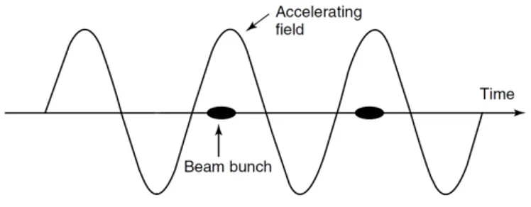
1.2 Proton LINACs VS electron LINACs 3 electromagnetic fields, usually in the VHF and UHF microwave frequency ranges. The accelerating structures are tuned to resonance and are driven by external, high-power RF tubes, such as klystrons, or various types of gridded vacuum tubes. The particles are launched inside the structure in bunchs and they are accelerated from the electric field excited inside the cavity, provided that the beam bunch is isochronous with the maximum accelerating filed along the LINAC, as shown in Fig. 1.1. The bunches may be separated longitudinally by one or more RF periods.
Fig. 1.1: Schematic of a particle bunch accelerated by an electric field.
1.2 Proton LINACs VS electron LINACs
One of the most famous linear accelerator for protons is the Drift Tube Linac (DTL), represented in Fig. 1.2: this long standing wave cavity can be divided into cell of different (increasing) lengths. The fields in all cells have the same phase so that the multicell structure can be said to operate in a 0-mode.
Fig. 1.2: Drift Tube Linac model.
Suppose we want to accelerate the beam to high energies in a long standing wave cavity. In order to work as an accelerator, the electric field must be along the direction of beam propagation. The beam must consist of bursts of particles with space in between the bursts. A burst of particles timed so as to see the accelerating portion
4 CHAPTER 1. INTRODUCTION of the field is called a "bunch". Typically, the electric field is driven by a sinusoidal voltage oscillating in time at the frequency of the cavity, see Fig. 1.3, and so the polarity of the electric field will be accelerating only half of the RF period (T /2), the rest of the time the field is oriented in such a way as to decelerate the beam. Thus, when alternating fields are used to accelerate particles, the beam cannot be a continuous stream of particles, for then half the particles would be decelerated instead of accelerated.
The solution has been proposed by Alvarez and consists to install hollow conduct-ing drift tubes along the axis, as shown in Fig. 1.3, into which the RF electric field decays to zero, as in a waveguide below the cutoff frequency. This creates field-free regions that shield the particles when the polarity of the axial electric field is opposite to the beam direction.
It is evident that, for a DTL structure, the maximum energy gain corresponds to the condition that a particle inside the bunch travels from one gap to the next in a time equal to T. In this case the particle will see an accelerating field in all the gaps. If we define the particle relativistic velocity as β = v
c with v the particle velocity and
c the speed of light, for a particle travelling at the relativistic velocity β, the time to cross one cell of length L is τ = L
βc. The condition τ = T gives the required cell
length for a 0-mode structure such as the DTL:
L = τ βc = T βc = βλ (1.1)
From this synchronism condition, it is clear that an electron LINAC, where the particles have β = 1 apart from a short initial section, will be made of a sequence of identical accelerating structures, with cells of the same length L = λ. The case of the proton LINAC is totally different, because β increases slowly by orders of magnitude, and the cell length has to follow a precise β profile: the cell length will increase as the particle travels along the structure.
As said before, the drift tubes allow us to divide the cavity into cells of length βλ extending from the center of one drift tube to the center of the next, as shown in Fig. 1.4.
For a DTL cell it is more practical to work with the average electric field E0:
it defined as the integral of the cell axial field E(z) along the cell axial length. The average voltage in every cell V0 varies with cell length βλ, and because V0 = E0βλ
in practice it is possible to tune a DTL that has constant E0 in every cell (but the
electric field in the gaps, E(z), will vary with cell geometry). The drift tubes are supported mechanically by stems attached to the outer wall, as seen in Fig. 1.4.
1.2 Proton LINACs VS electron LINACs 5
Fig. 1.3: Typical accelerating field of a metallic linear accelerator. Drift tubes are placed in the zones where a decelerating field would be otherwise present, creating a field-free region for travelling particles.
Fig. 1.4: Schematic of a DTL. The structure can be divided into cells, extending from the center of one drift tube to the center of the next. The cell length for a structure operating in the 0-mode (i.e. the distance from two drift-tube centers) is βλ, with β increasing as the particle travels along the structure. The drift-tubes are attached to the cavity outer wall through metal cylinders called ’stems’.
A body of mass m0, at rest with respect to an observer, represents a supply of
energy (called rest-mass energy or rest energy for short) given by W0, where W0 =
m0c2. Now let this mass be given some kinetic energy T , as by launching a particle
into an accelerator [1]. The total energy is
W = W0+ T ⇒ W = m0c2+ T (1.2)
By expressing the previous equation in terms of total mass, we obtain
6 CHAPTER 1. INTRODUCTION By remembering the relativistic statement for the mass as a function of velocity m = (1−v2m0/c2)1/2 it can be written T = m0c2 1 (1 − v2/c2)1/2 − 1 (1.4) if v is very small compared with c, this may be expanded in a power series in v/c
T = m0c2 1 + 1 2 v c 2 +3 8 v c 4 + · · · − 1 (1.5) and if the terms (v
c)
4, (v
c)
6, etc, are neglected, this reduces to
T = 1 2m0v
2 (1.6)
As long as the velocity is very small compared with that of light, the simple expression for kinetic energy is an adequate approximation of the truth, but it fails when the velocity is high, and the relativistic expression previously defined must be used because always correct. The relativistic expression for kinetic energy then becomes T = m0c2 1 (1 − β2)1/2 − 1 (1.7) and expressing it in terms of β yields to
β2= 1 − 1 1 + T
m0c2
2 (1.8)
The basic difference between electrons and ions [2] is their rest mass. The mass of an electron at rest is 9.1 × 10⁻³¹ kg while a proton has a mass of 1.6 × 10⁻²⁷ kg:
because of this mass difference, the two particles react differently when an RF field is applied inside the accelerating structure.
As said earlier, when accelerating particles the goal is to synchronize the acceler-ating field with the travelling particle in such a way that the particle sees the same field amplitude in each gap and thus it can be accelerated.
If we plot (1.8), β2 VS the gained kinetic energy (i.e. the distance along the
accelerator) for electrons (m0c2= 511 keV) and for protons (m0c2= 938 MeV) it can
be seen that the electrons come close to the speed of light already after few MeV of energy, and for the rest of the acceleration process their velocity will not change. The plot is shown in Fig. 1.5.
Instead, in a proton LINAC the particles have a slow increase in velocity as the energy increases. After reaching few GeV the velocity saturates towards c, well beyond
1.2 Proton LINACs VS electron LINACs 7
0 200 400 600 800 1000
Kinetic Energy (MeV) 106
0 0.2 0.4 0.6 0.8 1 1.2 2 = (v/ c) 2 electrons protons
Fig. 1.5: Relativistic particle velocity (protons and electrons) as function of gained kinetic energy.
the energy range of most proton linacs. That is the reason why, in a proton LINAC, an adaptation to the increase in particle velocity needs to be taken into account: this is usually made by increasing the cell length with the proton velocity.
Another difference between proton and electron LINACs is found in the type of structure being used for acceleration.
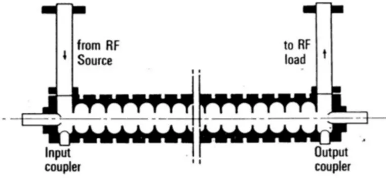
Travelling wave structures are generally used for electrons at β = 1 (see Fig. 1.6), designed to have phase velocity v = c for a given operating frequency. Input and output coupler are used to inject the RF wave and to extract at the end of the structure the remaining RF power. Electrons enters into the structure when the electric field is at its maximum and will travel along the LINAC with the same velocity as the wave, seeing the maximum accelerating electric field all along the structure and thus increasing their energy. The beam energy comes from the RF wave: part of the RF energy of the wave will be dissipated in the structure walls, usually made out of copper, part will be absorbed by the beam, and the rest will be extracted via the output coupler, to be absorbed in a matched load at the end of the structure.
8 CHAPTER 1. INTRODUCTION Travelling wave structures are designed for a fixed phase velocity, and can not be used for ions at β < 1. Even if the structure could be designed for a lower phase velocity corresponding to the initial β of the particles, when gaining energy the beam velocity would increase and the synchronism with the wave would be lost.
When dealing with protons, instead of matching the phase velocity of a travelling wave to the particle velocity, we can realize the synchronism between moving parti-cles and field by keeping constant the phase of the wave and by changing its space distribution accordingly to the synchronism condition. This is obtained in standing wave structures (RF cavities) like the DTL where the field is made 0 inside certain regions (the drift-tubes) as explained previously.
1.2.1 European Spallation Source (ESS) LINAC
The first part of this thesis deals with a proton accelerating structure and has been performed in the framework of the European Spallation Source (ESS).
The European Spallation Source (ESS) is a Research Infrastructure based in Lund (Sweden) with the vision to build and operate the world’s most powerful neutron source, enabling scientific breakthroughs in research related to materials, energy, health and the environment, and addressing some of the most important societal challenges of our time. This multi-disciplinary research centre will perform research that can potentially lead to the next great inventions within pharmaceuticals, envi-ronmental technology, energy, cultural heritage or fundamental physics.
Here, in particular the attention will be focused on the Drift Tube LINAC, which is a part of the entire ESS accelerating system as shown in Fig. 1.7. The DTL, cur-rently being assembled in the ESS Lund facility, is composed by 5 tanks working at 352.2 MHz with a constant average electric field of ∼ 3 MV/m; it can acceler-ate protons up to an energy of 90 MeV. This normal conducting accelerator creacceler-ates and accelerates the proton beam using room temperature structures. It is composed of matching sections as well as of accelerating components. The accelerating com-ponents have the particularity to adapt their geometry as the velocity of the beam increases making the acceleration very efficient (see §1.2). The DTL has a total length of ∼ 38 m and counts 175 cells: each cell possess a drift-tube, a supporting stem and a post-coupler for field stabilization if necessary (depending on the increasing length).
When simulating electrically large complex structures such as Drift Tube Linac (DTL) cavity in 3D simulators, it is important to choose a model representation that is a compromise between accuracy and time/resource cost: in the case of a DTL, the whole structure can easily reach a length of a few tens of meters, so a numerical
1.2 Proton LINACs VS electron LINACs 9
Fig. 1.7: Schematic of the ESS accelerating system.
representation problem is immediately evident. In fact, the simulation of such cavities, very complex in terms of geometry in particular due to the presence of the internal drift tubes and in general due to the presence of curved surfaces, can easily exhaust a high amount of computational resources in a very short time if the numerical problem is not smartly approached.
Usually an electromagnetic full-wave simulator makes convergence passes to reach the final solution: during a pass the model is meshed with a fixed number of tethrae-drons and, for each pass, the difference between two subsequent curves of S-parameters (the ∆S, used in driven modal problems) or two subsequent stored energy values (the ∆U , used in eigenmode problems) is calculated. The convergence is considered reached when, for two successive passes, these values are below a previously fixed value. The simulator will give results even if the convergence is not reached after a fixed number of passes, but especially for large electromagnetic structures, this will probably lead to high inaccuracies in terms of operating frequency and field results.
Possible ways to obtain accurate simulation results and at the same time to sim-plify a complex model in the way to obtain the desired convergence with the com-putational resources at disposal, is to exploit axial symmetries or to try to predict the mesh needed to have a specific frequency error. In the last case one can decide if that frequency error is good enough for the application at hand and, eventually, settle with that mesh and try to reduce the model complexity in an alternative way. The numerical techniques that allowed us to obtain quite good results in the process of simulating the tanks of the ESS DTL will be discussed in the next chapter. In Fig. 1.8 a DTL model with its mesh (HFSS simulation) is depicted.
1.2.2 Dielectric Laser Accelerators (DLA) and high gradient electron sources
The dielectric structures for electron acceleration that will be the argument of the second part of this thesis have been studied and developed in the DiElectric and METallic Radiofrequency Accelerator (DEMETRA) framework, a collaboration be-tween INFN-LNS, INFN-LNF, UniCT and UniBS. The experiment is dedicated to
10 CHAPTER 1. INTRODUCTION
Fig. 1.8: Drift Tube Linac HFSS simulation: the meshing elements (tethraedrons) used for the cavity representation are visible.
the modelling, development and test of RF structures devoted to acceleration that possesses high gradient of particles through metal and dielectric devices.
Due to electrical breakdown of metals in the presence of high electric fields, con-ventional particle accelerators, which consist of metal cavities driven by high-power microwaves, typically operate with accelerating fields from 10 to several dozens of MV/m. Because of the high power loss in metals at optical frequencies, dielectrics are the only viable candidate for confinement of the electromagnetic energy in such schemes. The DLA eliminate the issues of metallic accelerators when operating at high frequency, such as the power dissipation on the metallic walls, and allow the reaching of higher accelerating gradients (to the order of the GeV).
Dielectric laser acceleration with driving wavelengths in the optical and near-infrared region requires electron beams with normalized emittance of a few nanometers so that the beams can be fed into and kept inside the structure channel. In addition, for most applications, particularly for free-electron laser applications, high peak currents are mandatory, requiring high-brightness electron beams.
For electron beams, the source is a piece of conducting material that forms the cathode. Electrons are accelerated across the potential difference in the diode and emerge through a hole in the anode. The cathode may be either heated (thermal emission) or cold (field emission) or the electrons may be produced by photoemission. The beam brightness is defined as the number of particles, or the total beam current, with a given emittance [3].
For DLA the beam brightness is defined as [4]
Bn= B β2γ2 = 2I π2ϵ2 n (1.9)
1.3 Particle Acceleration in RF fields 11
where B is the geometric brightness, I is the electron bunch peak current, γ =
(1 − β2) and ϵ
n= βγϵ is the normalized emittance.
High gradient rf photo-injectors have been a key development to enable several applications of high quality electron beams. They allow the generation of beams with very high peak current and low transverse emittance, and in the past years photo-injectors with very good performances have been proposed [5].
1.3 Particle Acceleration in RF fields
Multicell ion LINACs are designed to produce a given velocity gain per cell. Particles that have the correct initial velocity will gain the right amount of energy to maintain synchronism with the field. Usually three phases can be defined: one for which the velocity gain is equal to the design value S, one earlier E and the last one later L than the crest of the accelerating wave inside the gap, as seen in Fig. 1.9.
Fig. 1.9: Early (E), stable (S), late (L) and unstable (U) particle phases.
The earlier phase is called the synchronous phase and is the stable operating point. It is a stable point because nearby particles that arrive earlier than the synchronous phase experience a smaller accelerating field, and particles that arrive later will ex-perience a larger field. This provides a mechanism that keeps the nearby particles oscillating about the stable phase, and therefore provides phase focusing or phase stability. The particle with the correct velocity at the stable phase is the synchronous particle, and it maintains exact synchronism with the accelerating fields. As the parti-cles approach relativistic velocities, the phase oscillations slow down, and the partiparti-cles maintain a nearly constant phase relative to the travelling wave. After beam injection into electron LINACs, the velocities approach the speed of light so rapidly that hardly any phase oscillations take place.
12 CHAPTER 1. INTRODUCTION The final energy of each electron with a fixed phase depends on the accelerating field and the value of the phase. In contrast, the final energy of an ion that undergoes phase oscillations about a synchronous particle is approximately determined not by the field, but by the geometry of the structure, which is tailored to produce a specific final synchronous energy. For an ion linac built from an array of short independent cavities, each capable of operating over a wide velocity range, the final energy depends on the field and the phasing of the cavities, and can be changed by changing the field, as in an electron linac.
1.3.1 Figures of merit of a linear accelerator
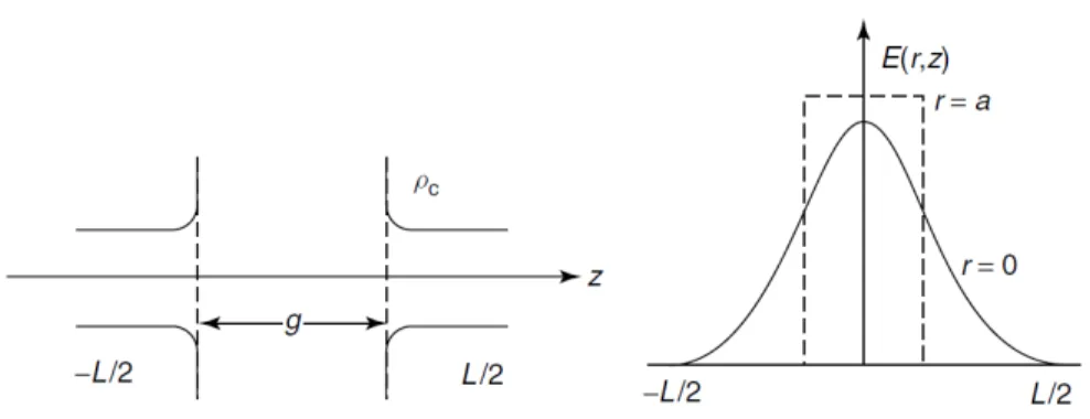
Let’s consider an accelerating gap as shown in Fig. 1.10. The electric field experienced by a particle travelling along the gap (radius r = 0) with a velocity v can be written as
Ez(r = 0, z, t) = E(0, z) cos(ωt(z) + φ) (1.10)
where t(z) =0zv(z)dz is the time at which the particle is found at the position z. Here we chose t = 0 when the particle is in the gap center and at this instant the phase of the field relative to the crest is φ.
Fig. 1.10: Accelerating gap of length g. The field inside the gap is also shown.
The energy gain of an arbitrary particle with charge q that travels through the gap is
∆W = L/2
−L/2
E(0, z) cos(ωt(z) + φ)dz (1.11) That, after the application of some trigonometry, can be written as
1.3 Particle Acceleration in RF fields 13
∆W = qV0T cos φ (1.12)
V0 =L/2
−L/2E(0, z)dz is the axial RF voltage. The quantity T is the transit time
factor, defined as T = L/2 −L/2E(0, z) cos ωt(z)dz L/2 −L/2E(0, z)dz − tan φ L/2 −L/2E(0, z) sin ωt(z)dz L/2 −L/2E(0, z)dz (1.13) Regardless of the phase φ, the energy gain of a particle in a harmonically time-varying field is always less than the energy gain in a constant dc field equal to that seen by the particle at the center of the gap. This is known as the transit-time effect, and the transit-time factor T is the ratio of the energy gained in the time-varying RF field to that in a dc field of voltage V0cosφ. Thus, T is a measure of the reduction in
the energy gain caused by the sinusoidal time variation of the field in the gap. Usually one can define an average axial accelerating field as E0 = V0L. V0 is the
voltage gain that would be experienced by a particle passing through a constant dc field equal to the field in the gap at time t = 0 and E0, which is an average field
over the length L, does depend on the choice of the latter. So, when a value of E0
is quoted for a cavity, it is important to specify the corresponding length L. For a multicell cavity, the natural choice for L is the geometric cell length.
If we call E0T the accelerating gradient, we can write the sometimes called
Panof-sky equation, that is the energy gain in terms of the average accelerating field
∆W = qE0LT cosφ (1.14)
Of course, the peak energy gain experienced by the particle occurs when it passes through the center of the gap, for φ = 0.
Usually E(z) is an even function about the geometric center of the gap. In this case the transit time factor expression simplifies as
T = L/2 −L/2E(0, z) cos ωt(z)dz L/2 −L/2E(0, z)dz (1.15) The transit-time factor increases when the field is more concentrated longitudinally near the origin, where the cosine factor is largest. Thus, the larger the gap between drift tubes and the more the field can penetrate into the drift tubes, the smaller the transit-time factor. The practice of constructing drift tubes with nose cones that extend further into the gap forces a concentration of the field near the center of the gap, and raises the transit-time factor.
By writing ωt ≃ ωz/v = 2πz
βλ, with βλ the distance that the particle travels in an
14 CHAPTER 1. INTRODUCTION T = L/2 −L/2E(0, z) cos( 2πz βλ)dz L/2 −L/2E(0, z)dz (1.16)
In order to characterize accelerating cavities, in the following some of the most important figures of merit will be defined.
For a metallic cavity with total stored energy U and average power loss on the walls P , one can define the well known cavity factor as
Q =ω0U
P (1.17)
We define the shunt impedance as an index of the effectiveness of producing an axial voltage V0 for a given power dissipated. It is usually expressed in MOhm.
rs=
V2 0
P (1.18)
Remembering that the maximum energy gain of the particle occurs when it is placed at the center of the gap (when φ = 0), the effective shunt impedance, a pa-rameter measuring the effectiveness per unit power loss in delivering energy to the particle, can be defined as
r = (∆Wφ=0 q ) 21 P = (V0T )2 P = rsT 2 (1.19)
For long cavities it is often preferable to use a figure of merit that is independent of both the field level and the cavity length L. Thus, it is also convenient to introduce shunt impedances per unit length
Z = rs L =
E2 0
P/L (1.20)
and the effective shunt impedances per unit length
ZT2= r L =
(E0T )2
P/L (1.21)
The last two usually are in the order of MOhm/m. Especially for normalconducting cavities, one of the main objectives in cavity design is to choose the geometry to maximize effective shunt impedance per unit length. This is equivalent to maximizing the energy gain in a given length for a given power loss.
In the case of a dielectric accelerator, a characteristic interaction impedance can be defined as [4], [6]
Zc=
(Eaccλ)2
1.3 Particle Acceleration in RF fields 15
and it is a measure of the effective accelerating field Eacc that acts on the
elec-trons for a given electromagnetic power flowing into the system P . As for metallic accelerators, high Zc values corresponds to a more efficient accelerator. The Zc is
distinguished from the shunt impedance rsof metallic accelerators because the latter
uses the power loss on the metallic walls instead of the power flowing into the system. A possible way to increase the interaction impedance in a dielectric accelerator is to use a material with high ϵror to properly tune the guiding channel practiced into the
dielectric.
For the dielectric accelerators an effective characteristic impedance can be defined in a similar fashion of that defined for metallic accelerators:
Z = (EaccλT )
2
P (1.23)
Part I
19
In the previous section the differences between proton and electron LINACs have been discussed. In the context of the ESS Drift Tube Linac realization, chapter 2 of this thesis deals with the analytical and numerical approaches used for the RF tuning of these large standing wave cavities, while chapter 3 presents the experimental results obtained with the realized cold model of the DTL tank 2. Finally, in chapter 4 a novel X-band structure for electron acceleration is presented and the experimental results obtained on a realized prototype are discussed.
2
Numerical study of metallic accelerators
In order to simulate the DTL cavities of the ESS LINAC, a set of representation methods have been developed. These methods, analytical and numerical, have the aim to find equivalent volumes in the way to simplify the simulation (i. e. to exploit rotational symmetry to simulate object slices) and, in conjunction or in alternative, to derive an analytic frequency error prediction formula, through structure symmetry exploitation, that ensures the required precision in real structure 3D representation, while using fair amount of computational resources. Both methods have been success-fully applied to design of the European Spallation Source (ESS) DTL cavities, now under construction.
2.1 Problem definition
3D simulators are becoming very useful nowdays, when a structure experimental tun-ing is required, to reduce the cost and time delay. When modelltun-ing complex structures in 3D FEM solvers, the real structure is discretized in a finite number of mesh ele-ments, usually tethraedrons. This results in an approximation of the real structure that in many situation introduces a systematic geometrical error as in the case of curved boundaries presence. In order to have a faithful description it is always possi-ble to have a finer and finer mesh by reducing the mesh size and increasing the mesh elements. However, computational resources impose a limit to this process.
A common choice/workaround to reduce the total number of mesh elements is to use simplified models (i.e. coarse mesh). Examples are mesh that neglect some geometric detail of the structure or mesh that follow curved or jagged boundary with low precision. A different approach is to use a2D reduced model exploiting symmetries, when present; in this case a virtually exact result is obtained with order-of-magnitude-less mesh elements. However, in general, simplified model may lead to inaccurate result if some important geometrical detail is lost or if the symmetry is only partially
22
CHAPTER 2. NUMERICAL STUDY OF METALLIC ACCELERATORS verified. Beside the possibility to work on a reduced computational domain, another approach to follow, also in combination with the above one, is to determine beforehand the appropriate geometric approximations to have both a minimum number of mesh elements and, at the same time, a numerical error below a fixed threshold. This scheme is very effective when compared to automated standard approach that refine the mesh during subsequent passes (i.e. with successive iterations until the required precision is reached). This automatic process is time consuming and, in general, may lead to mesh refinements also where not necessary.
In this section we apply a combination of the above discussed strategies: symmetry exploitation and predetermined geometric approximation. Through this section, as an example, we refer to a Drift Tube Linac (DTL) cell (see Fig. 2.3) but the methods have been successfully applied to the entire DTL tanks of the ESS project. Moreover the methodology is general; for instance, in [7] a similar approach is applied to a Radio Frequency Quadrupole accelerator (RFQ) as well.
The proposed method, presented in [8], allowed us to reach the correct simulation parameter to keep frequencies error below a prefixed threshold.
2.1.1 Symmetry and 2D reduced models
To exploit any symmetry problem to greatly reduce the total number of mesh elements while maintaining an accurate geometrical description is always a good choice.
Reflection (or mirror) symmetries [9], translational invariance [10] and rotational symmetries [11] can effectively reduce the computational domain and thus the size of the numerical problem.
For example it is well known that in a a × b rectangular waveguide the height b influences the waveguide loss but not other properties such as the cut-off frequency. This is due to the y-transnational in-variance of the fundamental mode TE10 and such property can be used in numerical simulations and also in practical realization of non standard wave-guides: examples are reduced-height waveguide to increase the mode overlap in launchers [12] and reduced-height waveguides in waveguide arrays to save physical space [13] or larger-height waveguides to accommodate higher power [14]. This y-invariance can be easily exploited also when solving numerical problems with PEC boundaries and no surface losses (with a huge reduction of the mesh size). In [10] this property has been applied to a finite conductivity rectangular waveguide by using a reduced computational domain while retaining an accurate prediction of the losses thanks to an appropriate correction factor.
2.1 Problem definition 23
(a) (b)
Fig. 2.1: 3D representation of a Drift Tube Linac cavity cell: (a) full structure and (b) slice.
Circular waveguides and rotational symmetric cavities such as the DTL cavity shown in Fig. 2.1(a) can also exploit a reduced 2D simulation domain with virtually exact simulation results. Moreover, differently than in the rectangular waveguide case, also the conductor losses are correctly predicted even if a small angular sector of the cavity is simulated without the need any correction factor (see Fig. 2.1(b)).
We will refer to the 3D simulation of a small angular sector as a quasi-2D simula-tion.
For a DTL cavity without stem it is actually possible to exploit the rotational symmetry of the geometry and to use a quasi-2D simulation in a small angular sec-tor of the full 3D-structure or even a 2D code cell representation. The resulting 2D (rotationally symmetric) problems can be solved with standard numerical approaches such as Finite Difference Time Domain (FDTD) and Finite Element Method (FEM). We used a code for 2D simulations, already available to the accelerator community, called Superfish [15], [16].
When, thanks to an exact symmetry, a 3D problem can be reduced to a 2D one without any approximation, the significant reduction of the problem dimension in term of mesh elements, makes possible to refine the mesh with standard brute force approach and to obtain rapidly converging results toward the “ideal” resonant fre-quency with small computational time. This frefre-quency value is virtually exact and can be considered as a reference for benchmarking the 3D simulations.
2.1.2 Curved surfaces and mesh
Fig. 2.2(a) shows the front view of a circular “pillbox” DTL cavity. When representing the structure using a 3D simulator such Ansys HFSS [17] the mesh engine creates a
24
CHAPTER 2. NUMERICAL STUDY OF METALLIC ACCELERATORS regular polygon mesh inscribed inside the cylindrical real structure. Whatever the mesh size/precision chosen, the simulated volume will be lower than the real cylin-drical volume. The more the mesh is coarse, the greater the geometrical error will be and thus the frequency and field errors will results, since the inscribed polygon fails to represent the real structure in a satisfactory and coherent way.
(a) (b)
Fig. 2.2: (a) Front view of a simulated circular cavity. Highlighted in red is the difference between real and simulated profile. (b) Circular sector of a cylindrical cavity.
Obviously, if the mesh density is increased, the real structure can be represented in a more accurate way and thus the simulated results will be more accurate. 3D simulators allow users to set the beginning mesh density, but for complex structures it is not straightforward to choose between a coarse mesh that could lead to inaccurate results, and an overly accurate mesh that could cost in resources and simulation time. When is possible to exploit the rotational symmetry and to perform 2D simula-tions, the above described error is not introduced because 2D rotations are analytically considered in the 2D formulation. However, as already discussed, when stems (in the case of a DTL cavity) or other geometrical details break the rotational symmetry, the cavity cannot be simulated with 2D codes (see Fig. 2.3).
2.2 Proposed approach
In a cavity at the resonance frequency f0, the stored electric and magnetic energies
are equal.
When the cavity is perturbed (in our case a perturbation will be either the stem or the coarse mesh on the outer wall) this will produce an unbalance of the latters and the frequency will shift to restore the balance [18], [19]. If this frequency shift is in relation with a coarse or incomplete description of the simulated geometry, it can
2.2 Proposed approach 25
(a) (b)
Fig. 2.3: Rotational symmetry and stem: (a) 3D and (b) side view of a DTL cell model. Central element is called drift tube and is attached to the cavity outer wall through a metal cylinder called stem. The presence of stem breaks axial rotation symmetry and this makes necessary full 3D simulations.
be considered as a frequency error on the simulated structure. From the theory we have [20], [18, Eq. (5.88), pag. 165], [19, Eq. (6.19), pag. 252]:
∆f0 f0 =∆ω0 ω0 = ∆V(µH 2− ϵE2)dV V(µH2+ ϵE2)dV = ∆Um− ∆Ue U (2.1) where ∆Um= 1 4 ∆V µH2dV (2.2) and ∆Ue=1 4 ∆V ϵE2dV (2.3)
are, respectively, the time average of the stored magnetic and electric energy re-moved by the perturbing object and
U =1 4
V
(µH2+ ϵE2)dV (2.4)
is the total stored energy inside the cavity.
We will use (2.1) to derive an analytical formula that can be employed to correct or predict the frequency error introduced by the structure discretization in the 3D simulator.
2.2.1 2D reference simulation
The first step was to simulate the 2D version of the DTL cell using Superfish simulator. Stem presence and its frequency effect are not directly considered in Superfish, but
26
CHAPTER 2. NUMERICAL STUDY OF METALLIC ACCELERATORS can be added later, directly within the code, through an automatic calculation based on Slater theorem (2.1).
Without the physical stem presence, we obtain an object that possesses a rotational symmetry and so we can use a very accurate mesh, located on the sheet of Fig 2.4(a), to obtain a virtually error free reference simulation.
In Fig 2.4(b) the accelerating electric field Ez on the cavity axis is also shown for
half cell. (a) 0 50 100 150 Length (mm) 0 2 4 6 8 10 12 Ez (MV/m) (b)
Fig. 2.4: (a) Superfish DTL cell representation. Thanks to the rotational symmetry, only half of the structure is actually simulated by using an extremely fine mesh. (b) Electric field Ez obtained for the considered cell.
2.2.2 3D curved boundaries and mesh error prediction
Fig. 2.2(b) shows how a generic tetrahedron edge approximate an actual curved boundary in 3D simulators.
The frequency error ∆f0 = f0− fmesh, where f0 is the correct cavity resonant
frequency while fmesh is the perturbed frequency of the 3D model, can be related to
the difference in volume ∆V between real profile and simulated one by using (2.1). It is clear that if a coarse mesh is used a large volume error is introduced. This “subtracted” volume, ∆V , is “large” at the outer DTL wall where the stored magnetic energy predominate, i.e. in the “subtracted” volume ∆Um≫ ∆Ueand then, by using
(2.2) on equation (2.1), one can write
∆f0 f0 = 1 4U ∆V µH2dV (2.5)
In order to calculate ∆V , we consider the cross section area difference between the real cavity profile and the simulated one, highlighted in red in Fig. 2.2(b), where the
2.2 Proposed approach 27
edge AB approximates the real circumference arc; the quantity α, known as normal deviation angle[1], is a specific curved mesh quality parameter that can be enforced
in Ansys HFSS to be lower than a fixed value in order to give a good geometrical approximation of the curved surfaces [17]. The objective of this section is to find an appropriate value of α that corresponds to a minimum but computationally reasonable frequency shift ∆f0. Then, by setting α, accurate electromagnetic results are obtained
in virtue of (2.5).
We call V the real cavity volume. After the numerical discretization the new vol-ume becomes Vmeshand we can define the quantity V −Vmesh= ∆V . The permittivity
ϵ and permeability µ of the medium are not varied and can be assumed constant. Also, we assume that the magnetic field, H, is constant inside ∆V . A case of particular in-terest occurs when the volume exhibits a cylindrical symmetry and the operational frequency f0corresponds to a mode with a little field variation along the axis. This is
the case of TM010 mode, which is typically used in RF cavities employed as elements
composing linear particle accelerators. In this case, if L is the cavity length and U the e.m. energy stored inside the cavity, by imposing ∆V = ∆AL equation (2.5) reads
∆f0
f0 ≃
1 4UµH
2∆AL (2.6)
where ∆A is the difference, referred to the circular cavity base, between the real profile and the discretized one. With reference to Fig. 2.2(b), let N = 2πα be the number of segments of the regular polygon inscribed inside the circle. So the precedent equation becomes ∆f0 f0 ≃ 1 4UµH 2∆A sN L (2.7)
where ∆As is the difference, referred to a circular sector, between real curved DTL
cross section area and the discretized cross section.
From Fig. 2.2(b), it can be seen that ∆As = As1− As2. As1 is the area of the
circular sector and As2is the area of triangle AOB.
• For the calculation of As1, we know that
Asector: Acircle= angsect: 2π (2.8)
so
As1=
R2α
2 (2.9)
where R is the cavity (circle) radius.
[1] The normal deviation angle is defined as the maximum angular deviation between the
28
CHAPTER 2. NUMERICAL STUDY OF METALLIC ACCELERATORS • For the calculation of As2we can consider it the sum of two small triangles. Let’s
take the AOC one:
OA = R (2.10) AC = R sinα 2 (2.11) OC = R cosα 2 (2.12) Then As22 is As2 2 = R2 2 sin α 2 cos α 2 = R2 4 sin α −→ As2= R2 2 sin α (2.13) Therefore we obtain ∆As=R 2 2 (α − sin α) (2.14)
Substituting (2.14) into (2.7) we obtain ∆f0 f0 ≃ 1 4UµH 2αR2 2 (1 − sin α α )N L = = 1 4UµH 2πR2(1 −sin α α )L (2.15)
and so, by imposing α inside the previous equation, the frequency error ∆f0due to 3D
circular structure representation can be controlled and minimized, of course keeping also in mind the computational resources available.
It is clear that (2.15) requires the knowledge of the field H at the point where the volume is subtracted. In our case this value can be determined through a 2D simulation, as a reference.
2.3 Numerical validation
2.3.1 Mesh error prediction formula application
In the following section we test equation (2.15) on the DTL cell (see Fig. 2.3). The cell has the following specifications, obtained by using a 2D Superfish simulation taken as reference (as described in §2.2.1) and by considering a mean accelerating field E0 = 3.04 MV/m inside it: U = 0.81 J, total stored energy inside the cell,
R = 0.2605 m, cell radius, H = 3745 A/m, average magnetic field on the cavity outer wall, L = 0.289 m, cell length, f0= 351.266 MHz, cell operating frequency taken as
ground truth.
The frequency error calculation procedure can be summarized as follows: 1. obtain all the needed global specifications with an accurate 2D simulation;
2.3 Numerical validation 29
2. insert these reference values, obtained with the 2D simulation, inside equation (2.15) and derive some α values in the way to obtain the estimated frequency error ∆f0;
3. when a satisfactory ∆f0 is chosen (depending on structure tolerances and
appli-cation) impose the corresponding α value in the 3D simulation in order to obtain electromagnetic results with a controlled frequency error;
4. if the selected α value leads to unreasonable heavy 3D simulation, repeat the previous step with relaxed precision requirements (higher α value, worse 3D rep-resentation).
In Table 2.1, for different values of αi, we report the value of fmesh= f0+ (∆f0)i
estimated through the semi-analytical formula (2.15) and the correspondent results from full wave HFSS simulations. The agreement is very good.
Table 2.1: DTL cell resonant frequency f0obtained through analytical calculation and HFSS
simulation for different values of α.
αi fi (analytical) (MHz) fi(HFSS) (MHz)
10◦ 351.88 351.72
5◦ 351.42 351.272
In Fig. 2.5 the difference in mesh between the use of α = 10◦ and α = 5◦ can be
observed. The bad representation of the cavity outer wall obtained by using a coarse mesh lead to an unacceptable frequency error and will have an impact on the overall DTL tank simulation both in terms of frequency and field precision.
2.3.2 Equivalent volume method
As stated before, the cavity stem breaks the rotational symmetry and causes a fre-quency error with respect to the real one. This error can be predicted as detailed in §2.3.1 and a countermeasure can be applied in terms of mesh utilization to represent the model.
A possible alternative approach could be the use of an equivalent stem volume that introduces the same frequency shift without breaking the rotational symmetry [21].
The method adopts a model representing the DTL cell with a “modified stem volume” that correctly accounts for the frequency shift but, not breaking the rotational symmetry, also allows the use of periodic boundary condition to simulate only a cell slice instead of the entire structure. This equivalent volume can be found by relating
30
CHAPTER 2. NUMERICAL STUDY OF METALLIC ACCELERATORS
(a) (b)
Fig. 2.5: (a) HFSS cell front face mesh using α = 10◦. (b) HFSS cell front face mesh using
α = 5◦
the magnetic field at the point where it is subtracted with the average field along the real stem.
Both the real and virtual stem lay in a region with low electric field, E, so the following reasoning is made considering only the unbalance in magnetic field, H, and in particular to correct the frequency shift we require:
∆Vreal stem µH2dV = ∆Vvirtual stem µH2dV that can be approximated as
∆S ∆Lreal stem µH2dL =Hline−avg∆L = ∆Vvirtual stem µH2dV =HV −avg∆V
(∆S∆L)real stemHline−avg ≈ (∆V )virtual stemHV −avg
Let’s consider Fig. 2.3: here a real stem of radius r = 14 mm and height ∆L = 215.5 mm is inserted. If we calculate the average magnetic field along its height, we have a value of Hline−avg ≃ 1194 A/m. The rotational symmetric volume that will represent the real stem could be of any form: for simplicity, let’s take a simple triangular area and consider a volume obtained by rotating this area around the cell axis. As second step, by knowing that in a DTL cell the magnetic field has its maximum concentrated practically only in the center of the drift tube outer wall at coordinates r = rDT, z = L/2 (or z = −L/2, see reference system of Fig. 2.3), a
simulation has been performed and it has been found that a proper magnetic field value at these coordinates is HV −avg= 9417 A/m. The objective of this method is to
2.3 Numerical validation 31
find the exact dimensions of the “equivalent volume” in the way that, when weighted with HV −avg, it has the same frequency effect of the real stem volume weighted with
Hline−avg, that is:
(∆V )virtual stemHV −avg
πr2H line−avg
= 1 (2.16)
Solving (2.16), we obtain (∆V )virtual stem≃ 78000 mm3. Now, by arbitrarily fixing
the triangle height h = 25 mm, by simple mathematical steps the triangle base can be determined in the way to obtain the proper triangle volume. In our case, the determined triangle base is b = 9.3 mm and, by making a full 3D simulation with these volumes as shown in Fig. 2.6, we found an operating frequency f0= 351.276 MHz
that is in excellent agreement with that found with the mesh error prediction formula and reported in Table 2.1 for α = 5◦.
The application of the equivalent volume method has been applied on the DTL cell in a HFSS simulation, but the method can also be applied in 2D simulations.
Fig. 2.6: Application of the equivalent volume method to half DTL cell in HFSS. A normal deviation angle of α = 5◦ is also used to ensure accurate results.
NOTE: in the application of this method one has to be careful when inserting the equivalent volume. In the case of the DLT cell we are interested only in the accelerating on axis electric field, that is mainly located between the two drift tube halves. So, the electric field is not affected from the insertion of a triangular solid equivalent volume instead of the real stem. But this could not be the case if one considers different geometries.