ISSN 2282-6483
Measuring Global
Macroeconomic Uncertainty
Graziano Moramarco
Quaderni - Working Paper DSE N°1148
Measuring Global Macroeconomic Uncertainty
Graziano Moramarco∗University of Bologna
June 11, 2020
Abstract
This paper provides new indices of global macroeconomic uncertainty and investigates the cross-country transmission of uncertainty using a global vector autoregressive (GVAR) model. The indices measure the dispersion of forecasts that results from parameter un-certainty in the GVAR. Relying on the error correction representation of the model, we distinguish between measures of short-run and long-run uncertainty. Over the period 2000Q1-2016Q4, global short-run macroeconomic uncertainty strongly co-moves with fi-nancial market volatility, while long-run uncertainty is more highly correlated with eco-nomic policy uncertainty. We quantify global spillover effects by decomposing uncertainty into the contributions from individual countries. On average, over 40% of country-specific uncertainty is of foreign origin.
Keywords: global uncertainty, uncertainty index, GVAR, spillovers, bootstrap JEL classification: C15, C32, E17, D80, F44, G15
∗Email: [email protected]; [email protected]. I would like to thank Piergiorgio
Alessandri, Giuseppe Cavaliere, Flavio Cocco, Luca Fanelli, Carlo Favero, Mario Forni, Roberto Golinelli, Paolo Manasse, Antonio Ribba, Barbara Rossi and participants at the 8th Italian Congress of Econometrics and Empirical Economics (Lecce, 2019), the 68th Annual Meeting of the French Economic Association (Or-léans, 2019), the BOMOPAV Economics Meeting (Modena, 2019) and the 6th SIdE-IEA Workshop for PhD students in Econometrics and Empirical Economics (Perugia, 2018) for useful comments and suggestions. The usual disclaimer applies.
Non-Technical Summary
The world economy has been burdened by substantial uncertainty in recent years. Following
the global financial crisis of 2007-2009, economists have increasingly studied uncertainty and
its effects. For this purpose, they have relied on a variety of uncertainty measures, ranging
from stock market volatility to disagreement among professional forecasters, from keywords
in newspaper articles to the probability distributions of shocks in econometric models. Still,
the global dimension and the cross-country transmission of uncertainty remain largely
un-explored. Also, the disconnect between different measures of uncertainty (in particular, between economic policy uncertainty and financial market volatility) has puzzled economists
and market participants.
In this paper, we deal with such issues. We develop quarterly indices of global
macroe-conomic uncertainty and study the transmission of uncertainty using a global vector
au-toregressive (GVAR) model (Pesaran et al. 2004), which is a high-dimensional econometric model commonly used to investigate economic and financial interconnections between
coun-tries. More specifically, we estimate the time-varying uncertainty about the parameters of
the GVAR model and measure its effects in terms of forecast uncertainty. The resulting
indices of uncertainty are comprehensive, as they cover 20 advanced and emerging economies
(33 countries), accounting for about 80% of world GDP, and use information from a set
of key macroeconomic variables, both real and financial (real GDP levels, inflation rates,
short-term interest rates, exchange rates and stock market indices), from 1979Q1 to 2016Q4.
From a methodological point of view, the proposed approach allows to capture both global
uncertainty shocks (common to all countries) and the global propagation of country-specific
shocks (i.e., contagion effects).
At the same time, the paper distinguishes uncertainty on short-run economic dynamics,
on the one hand, and uncertainty on the long-run economic equilibrium, on the other. The results suggest that such distinction helps reconcile measures of financial market uncertainty
and economic policy uncertainty over the period 2000Q1-2016Q4. In particular, the proposed global short-run macroeconomic uncertainty (GSRMU) index shows a strong co-movement
with the VIX index of stock market volatility, while the global long-run macroeconomic
uncertainty (GLRMU) index is more highly correlated with the economic policy uncertainty
(EPU) index by Baker, Bloom and Davis(2016).
Importantly, the paper estimates the global spillovers of uncertainty by disentangling
the domestic and international sources of uncertainty in each country. On average, foreign
uncertainty is found to account for more than 40% of individual countries’ uncertainty. The
Euro Area and the United States generate the highest global spillovers in terms of short-run
uncertainty, while China is the largest source of long-run uncertainty. The countries that
receive the highest spillovers from the rest of the world are Canada, Sweden and
Switzer-land, while uncertainty in China and South-East Asia has a comparatively large domestic
1 Introduction
Economic uncertainty has been a major concern at a global level for more than a decade. It is
often mentioned among the factors that slow down economic activity (e.g.,ECB 2009;Stock and Watson 2012; Bloom et al. 2012) and its international transmission plays a key role in shaping macroeconomic outlooks (e.g., IMF 2012). Following the global financial crisis of 2007-2009, economists have relied on a variety of methodologies to measure uncertainty and
study its effects (see, e.g.,Bloom 2014;ECB 2016). Still, the global dimension and the cross-country transmission of uncertainty remain largely unexplored. On the one hand, several indicators of uncertainty have been constructed for a large number of countries separately,
without investigating the interconnections between countries (e.g., Baker, Bloom and Davis 2016; Scotti 2016; Ozturk and Sheng 2018; Ahir, Bloom and Furceri 2018). On the other hand, existing approaches based on multi-country models (Berger et al. 2017; Mumtaz and Theodoridis 2017;Mumtaz and Musso 2019;Carriero et al. 2020; Crespo Cuaresma, Huber and Onorante 2019) focus on identifying common components of uncertainty across countries and are not designed to study the global propagation of country-specific uncertainty shocks
(i.e., contagion effects). Also, they are typically limited to advanced economies.
A second problem with existing proxies of uncertainty is that they show remarkable
differ-ences between each other. In particular, the disconnect between measures of economic policy
uncertainty (such as the EPU index byBaker et al. 2016) and stock market volatility (such as the VIX) has puzzled market participants and policymakers in recent years (ECB 2017; Pas-tor and Veronesi 2017). More generally, economic uncertainty is known to be a multifaceted concept (Bloom 2014;Forbes 2016) and its different proxies need to be reconciled.
This paper deals with such issues. It provides new quarterly measures of global
macroe-conomic uncertainty and investigates the cross-country transmission of uncertainty by means
of a global vector autoregressive (GVAR) model (Pesaran et al. 2004). The global uncertainty indices are comprehensive, as they take into account the economic interconnections between
20 advanced and emerging economies (33 countries), representing about 80% of world GDP, and use information from both real and financial variables (real GDP levels, inflation rates,
short-term interest rates, exchange rates and stock market indices), from 1979Q1 to 2016Q4.
The approach captures both global uncertainty shocks and the international propagation of
country-specific shocks. Importantly, the paper quantifies global uncertainty spillovers by
disentangling the domestic and international sources of uncertainty in each country. On
average, foreign uncertainty is found to explain more than 40% of individual countries’
un-certainty.
At the same time, the paper distinguishes uncertainty on short-run economic dynamics, on
the one hand, and uncertainty on the long-run economic equilibrium, on the other, using the
error correction representation of the GVAR model. The results suggest that such distinction
helps reconcile financial market uncertainty and economic policy uncertainty in recent years,
in line with the findings of Barrero et al. (2016). In particular, over the period 2000Q1-2016Q4 the global short-run uncertainty (GSRMU) index has a correlation of 0.8 with the
VIX index of stock market volatility (and 0.66 with the macro uncertainty index by Jurado, Ludvigson and Ng 2015), while the long-run uncertainty index (GLRMU) is more highly correlated with the economic policy uncertainty (EPU) index by Baker, Bloom and Davis
(2016): in this case, the correlation between global indices is 0.35 and the correlation between U.S.-specific indices is 0.59.
Uncertainty is measured as the dispersion of forecasts that results from parameter
uncer-tainty in the GVAR model. FollowingDées et al.(2007a,b), we estimate the distributions of GVAR parameters by bootstrapping. We track parameter uncertainty over time by iterating
a bootstrap procedure across recursive sample windows. In each window, (i) the distribution
of parameters is estimated by a non-parametric bootstrap, (ii) parameter uncertainty results
into distributions of (pseudo-)out-of-sample forecasts and (iii) the standard deviation of
forecasts become less reliable estimates of the expected future values of variables.1 Since cross-country economic linkages are explicitly modeled in the GVAR, all variable-specific
measures of uncertainty across the world economy are interdependent and consistent with
each other.
Variable-specific uncertainties are aggregated into country-level indices to provide
com-prehensive measures of macroeconomic uncertainty. The indices turn out to be highly
cor-related with each other, indicating that macroeconomic uncertainty is largely shared across
countries in the global economy. Such commonality is the result of two factors: global shocks,
reflected in the correlations of parameters across countries, and the transmission of
country-specific shocks (contagion effects), ensured by the dynamic relationships between countries in
the GVAR. Finally, global indices are computed as weighted averages of the country-specific
indices, using GDP levels at purchasing power parity (PPP) as weights.
Global spillovers of uncertainty are measured by calculating the contribution of each
country to other countries’ macroeconomic uncertainty. To estimate the spillovers, we use
bootstrap simulations in which parameter uncertainty is either selectively “switched off” or
“switched on” for one country-specific model at a time. On average, uncertainty of foreign
(non-domestic) origin accounts for 41% of domestic short-run uncertainty and 56% of
long-run uncertainty. The economies that generate the highest global spillovers are the Euro Area, the United States, China and South-East Asia. The countries that receive the highest
spillovers from the rest of world are Canada, Sweden and Switzerland, while uncertainty in
China and South-East Asia shows a comparatively large domestic component.
A thriving literature has investigated fluctuations in uncertainty and developed methods
to measure it. Some of the proposed proxies are based on observables, such as indices of
option-implied stock market volatility (Bloom 2009), distributions of survey forecasts and forecast errors (Lahiri and Sheng 2010; Bachmann, Elstner and Sims 2013; Rossi and
Sekh-1In this respect, using a high-dimensional model with a limited amount of restrictions, such as the GVAR,
posyan 2015, 2017; Scotti 2016; Ozturk and Sheng 2018) or the frequency of newspaper articles containing specific sets of words (Baker et al. 2016). To address the limitations of observable measures (see, e.g., Lahiri and Sheng 2010; Coibion and Gorodnichenko 2012), model-based measures of uncertainty have also been proposed, typically using factor models
with stochastic volatility. In a seminal paper, Jurado, Ludvigson and Ng (2015) measure uncertainty in the United States through a factor-augmented vector autoregression, using a
large dataset of monthly macro and financial indicators. Berger, Grabert and Kempa(2016,
2017), Mumtaz and Theodoridis (2017) and Mumtaz and Musso (2019) use multi-country factor models with stochastic volatility to decompose uncertainty in OECD countries into
common and country-specific components. Using U.S. data, Carriero, Clark and Marcellino
(2017) jointly estimate uncertainty and its impact on the economy through a large VAR in which stochastic volatility is driven by common factors. Carriero, Clark and Marcellino
(2020) andCrespo Cuaresma, Huber and Onorante(2019) use large Bayesian VARs to mea-sure uncertainty and its effects in 19 industrialized economies and G7 countries, respectively.
We highlight the contributions of this paper compared to related studies. First, to our
knowledge this is the first paper that provides measures of global macroeconomic uncertainty
and global spillovers of uncertainty using a GVAR model. Among the existing approaches for
measuring international uncertainty, Mumtaz and Theodoridis(2017), Berger et al.(2017),
Mumtaz and Musso (2019), Carriero et al. (2020) and Crespo Cuaresma et al. (2019) use different models, do not consider emerging economies and do not deal with the propagation
of uncertainty from one country to the others. Ozturk and Sheng (2018) develop a com-prehensive index of global uncertainty using survey forecast data, but do not model global
economic interrelations nor analyze the international transmission of uncertainty. Ahir, Bloom and Furceri (2018) construct an index of uncertainty for 143 individual countries using the frequency of the word “uncertainty” in the quarterly Economist Intelligence Unit
country reports. Rossi and Sekhposyan (2017) investigate spillovers of output growth- and inflation-based uncertainty using survey data for the Euro Area, while Klößner and Sekkel
(2014) estimate spillovers of policy uncertainty among six developed countries using the EPU index by Baker et al. (2016).
Second, the paper develops distinct measures of short-run and long-run uncertainty.2
More specifically, short-run uncertainty is measured as the standard deviation of forecasts
conditional on the long-run parameters of the model. Accordingly, it is quantified by
com-puting bootstrap distributions of the short-run parameters of the GVAR while fixing the
long-run parameters at their maximum likelihood estimates. Instead, long-run uncertainty is
measured as the dispersion of forecasts when all parameters in the global model are treated as
uncertain.3 The results suggest that financial market volatility over the last two decades can
be associated with uncertainty on the short-run dynamics of the economy, while the observed
increases in policy uncertainty have been mostly related to the long-run consequences of the
global financial crisis and the Euro area crisis.
Third, unlike other model-based approaches for measuring uncertainty (Jurado et al. 2015;
Berger et al. 2017; Mumtaz and Theodoridis 2017), this approach estimates uncertainty in
2The economic literature suggests at least three reasons why the distinction between short-run and long-run
uncertainty may be relevant. First, the relative importance of short-run as opposed to long-run unpredictabil-ity arguably varies across economic agents. For instance, “financial risk management has generally focused on short-term risks rather than long-term risks” (Engle 2011). On the other hand, long-run uncertainty is central to a number of policy issues. For instance, uncertainty about potential (long-run) output affects the reliability of the output gap estimates, which are key inputs for both fiscal policy and monetary policy (Orphanides and van Norden 2002). Also, reducing uncertainty about long-run inflation and interest rates is often seen as criti-cal for the effectiveness of monetary policy (Bernanke 2007;Gürkaynak et al. 2005;Orphanides and Williams 2005). Second, forecasters may be not equally exposed to these two types of uncertainty, depending on the specification of their forecasting models. As documented by the literature on cointegration, modeling long-run economic relationships is not always beneficial for forecast performance (see, for example, Hoffman and Rasche 1996;Lin and Tsay 1996), which means that it may be reasonably omitted in many contexts. Third, the effects of short-run and long-run uncertainty on economic activity may differ. For instance, investment may be more responsive to long-run than to short-run uncertainty (Barrero et al. 2016).
3Cf. Barrero et al. (2016), where the distinction between short run and long run relates to the forecast
a given period without using data on subsequent periods (except for mere standardization). Accordingly, it is fully suitable for use in real time.
Fourth, the paper focuses on parameter uncertainty as a source of forecast uncertainty.
The aim is to provide measures that are conceptually closer to Knightian (or radical)
un-certainty than to risk, as parameter unun-certainty undermines individuals’ confidence in the
estimated probability distributions of economic outcomes. Conversely, measuring uncertainty
with the estimated volatility of shocks, as is often done in the literature4, implicitly relies on
the assumption that the probability distributions can be treated as known, which pertains
more to the concept of risk.5
Finally, the paper contributes of course to the GVAR literature. Cesa-Bianchi, Pesaran and Rebucci (2014) use a GVAR model to study the relationship between uncertainty and economic activity. Unlike in this paper, however, they do not compute GVAR-based measures
of uncertainty, but use observed proxies (asset price volatility) as an input to the model. Dées et al.(2007a,b) apply bootstrap methods to the GVAR in order to obtain confidence intervals of impulse response functions and log-likelihood ratio tests for over-identifying restrictions,
not to construct indices of time-varying uncertainty. Also, unlike these authors, we obtain
key results by implementing different versions of the bootstrap algorithm and extend the
bootstrap to account for uncertainty about cointegration ranks.
4An exception isOrlik and Veldkamp(2014), who focus on parameter uncertainty in a univariate model
for U.S. GDP.
5Moreover, the literature has emphasized the importance of parameter uncertainty in several contexts. In
a seminal paper,Brainard(1967) showed that parameter uncertainty affects policymakers’ optimal choices, whereas uncertainty about error terms can be ignored when setting policy variables, under standard quadratic objective functions. A subsequent literature has expanded on the implications of parameter uncertainty for monetary policy (e.g., Wieland 2000; Söderström 2002). Theoretical models with parameter uncertainty and learning have been proposed to improve on rational expectations models by accounting for key macro puzzles, such as the equity premium puzzle (Hansen 2007; Collin-Dufresne et al. 2016; Weitzman 2007). In finance, parameter uncertainty affects the relationship between the investment horizon and the optimal portfolio allocation (Xia 2001).
The remainder of the paper is organized as follows. Section 2 presents the methodology used to measure uncertainty and its spillovers. Section3presents the empirical implementa-tion and the results. Secimplementa-tion4 concludes.
2 The Econometric Framework
This section illustrates the methodology used to measure global macroeconomic uncertainty,
distinguish short- and long-run uncertainty and capture cross-country uncertainty spillovers.
2.1 The GVAR model
The GVAR model (Pesaran et al. 2004) results from the aggregation of country-specific VARX* models, in which domestic macroeconomic variables are related to their foreign
counterparts. To reduce the dimensionality of the parameter space, the foreign variables are
built as cross-country weighted averages, using weights based on international trade flows.
These foreign aggregates are treated as weakly exogenous in each VARX*, which implies that
the estimation is performed at the country level. The GVAR model is estimated on quarterly
data.
Let xitdenote the ki× 1 vector of domestic macroeconomic variables of a generic country
i at time t, with i = 1, ..., N , where N is the total number of countries. Let x∗it denote the
ki∗× 1 vector of foreign variables. The VARX* model for country i can be written as:
xit = a0i+ a1it + pi ∑ j=1 Φjixi,t−j+ qi ∑ l=0 Λlix∗i,t−l+ νit (1)
where a0i and a1i are ki × 1 vectors of constants and trend coefficients, respectively, Φji, for j = 1, . . . , pi, and Λli, for l = 0, 1, . . . , qi, are ki× ki and ki× ki∗ matrices of parameters, respectively, and νit∼ iid(0, Σi) is the vector of errors. In the GVAR literature, quarterly VARX* models typically include one or two lags of the domestic and foreign variables (e.g.,
Pesaran et al. 2004; Dées et al. 2007a). In this paper, two lags are included for all variables and all countries, i.e., pi= qi = 2 for every i.
Let k be the total number of endogenous variables in the global economy, i.e., k =∑N i ki. Domestic and foreign variables can be expressed in terms of the k×1 stacked vector of global endogenous variables xt: xit x∗it = Wi x1t x2t .. . xN t = Wixt (2)
where Wi is the (ki+ ki∗)× k matrix of country-specific trade-based weights.
The error correction representation of the country-specific model, or VECX*,
distin-guishes long-run (cointegrating) relationships between variables and short-run dynamics.
Defining zit= (x′it, x∗it′)′, it can be written as:
∆xit = ¯a0i− Πi[zi,t−1− γi(t− 1)] − Φ2i∆xi,t−1+ Λ0i∆x∗it− Λ2i∆x∗i,t−1+ νit (3)
where Πi is a ki× (ki+ k∗i) matrix of parameters, ¯a0i is a ki× 1 vector of constants and γiis a (ki+ k∗i)× 1 vector of trend coefficients. Given (1), a0i= ¯a0i− Πiγi and a1i = Πiγi. The rank ri of matrix Πi represents the number of long-run relationships between the variables
in zit. In particular, Πi = αiβ′i, where αi is the ki × ri matrix of loadings and βi is the (ki+ ki∗)×ri matrix of cointegrating vectors (seeJohansen 1995). Also, given (1) it is readily seen that Πi= ( Iki− ∑2 j=1Φji,− ∑2 l=0Λli )
, where Iki is the ki× ki identity matrix.
Stacking all country-specific VARX* models provides a vector autoregressive representa-tion of the global economy:
where a0 = (a0′1, a02′,· · · , a0′N)′ and a1 = (a1′1, a1′2,· · · , a1′N)′ are the k × 1 vectors of stacked global constants and trends, respectively, νt= (ν′1t, ν′2t,· · · , ν′N t)′ is the k× 1 vector of stacked errors and:
G = (Ik1,−Λ01) W1 (Ik2,−Λ02) W2 .. . (IkN,−Λ0N) WN , H1= (Φ11, Λ11) W1 (Φ12, Λ12) W2 .. . (Φ1N, Λ1N) WN , H2 = (Φ21, Λ21) W1 (Φ22, Λ22) W2 .. . (Φ2N, Λ2N) WN (5)
The reduced form of the global model can be written as:
xt= c0+ c1t + F1xt−1+ F2xt−2+ εt (6)
where:
c0 = G−1a0, c1 = G−1a1,
F1 = G−1H1, F2 = G−1H2
(7)
and εt= G−1νt is the vector of reduced-form global errors.
Finally, it is useful to express the model in companion form: xt xt−1 = c0 0 + c1 0 t + F1 F2 Ik 0 xt−1 xt−2 + εt 0 (8)
In what follows, the companion form will be denoted as:
˜
2.2 Time-varying uncertainty
To derive time profiles of short- and long-run uncertainty using the GVAR model, we employ
a non-parametric bootstrap procedure (cf. Dées et al. 2007a,b).6 The procedure consists of
the following steps:
1. The GVAR is estimated across recursive sample windows. The shortest window goes
from time 1 to, say, time T0, then the sample is extended by one-quarter increments up
to [1, Tmax], where Tmax identifies the last observation in the dataset. To estimate the
country-specific VECX* models on each window, window-specific foreign variables are constructed using trade data that were available in the final quarter of the window under
consideration (Section 3 provides more details on this). Let us consider the maximum-likelihood estimate of the GVAR obtained using actual data up to a given quarter. In the
generic window w ending in period Tw, the maximum-likelihood GVAR is expressed as:
xt=bc (w) 0 +bc (w) 1 t + bF (w) 1 xt−1+ bF (w) 2 xt−2+bε (w) t (10)
where the b symbol denotes estimates and t = 1, 2, . . . , Tw.
2. In each sample window, a non-parametric bootstrap of the estimates is performed. First,
we simulate alternative historical paths for all the variables in the global model within the
sample window, using the maximum-likelihood GVAR (10) and the empirical distribution of the errors. Then, we re-estimate all the VECX* models and, consequently, the global
6Dées et al.(2007a,b) compute bootstrap distributions of the GVAR parameters, but not of the
cointe-gration ranks. As shown below, we extend the bootstrap to account for uncertainty about the number of long-run relationships. In the context of VAR models,Cavaliere et al.(2012) have established that bootstrap inference on cointegration ranks is asymptotically valid when the bootstrap samples are constructed using the restricted parameter estimates of the VAR obtained under the reduced rank null hypothesis, which is what we do in this paper. Proofs of the validity of bootstrap tests of hypotheses on cointegrating vectors and adjustment coefficients are provided inBoswijk et al.(2016).
model on the simulated time series.
More specifically, in window w:
(a) The window-specific maximum-likelihood GVAR estimate (10) produces a k× Tw matrix of global residuals bE(w) =
( bε(w) 1 ,bε (w) 2 , . . . ,bε (w) Tw−1,bε (w) Tw ) .
(b) In the generic b-th bootstrap iteration, with b = 1, . . . , B, the Tw columns of
ma-trix bE(w) are resampled. Then, artificial time series are generated for all the vari-ables through an in-sample simulation of model (10) using the resampled residuals as shocks. Denoting iteration b in window w with the superscript (w, b), let ε(w,b)t be
the bootstrap shocks, generated by randomly drawing columns from bE(w) (thereby preserving the cross-sectional covariances) with replacement. The simulated time
series are given by:
x(w,b)t =bc(w)0 +bc(w)1 t + bF(w)1 x(w,b)t−1 + bF(w)2 x(w,b)t−2 + ε(w,b)t (11)
with x(w,b)0 = x0 and x(w,b)−1 = x−1.
Iteration-specific foreign variables x∗(w,b)it are then constructed using the
window-specific trade weight matrix W(w)i for every i.
(c) In each bootstrap iteration, all the VECX* models are re-estimated on the simulated
data. Two cases are considered:
i. Uncertainty is measured on short-run parameters only. In this case, short-run
parameters are re-estimated in each iteration while the long-run vectors βi and
γi are fixed at their maximum likelihood estimates bβ(w)i and bγ(w)i across all iterations (and the cointegration rank is fixed at br(w)i ), i.e.:
∆x(w,b)it = b¯a(w,b)0i − bα(w,b)i βb(w)i ′ [ z(w,b)i,t−1− bγ(w)i (t− 1) ] + − bΦ(w,b)2i ∆x(w,b)i,t−1+ bΛ(w,b)0i ∆x∗(w,b)it − bΛ(w,b)2i ∆x∗(w,b)i,t−1 +bν(w,b)it (12)
ii. Both short-run and long-run parameters are treated as uncertain. Accordingly, all parameters are re-estimated in each iteration, also allowing for
iteration-specific cointegration ranks r(w,b)i (details on rank selection are provided below):
∆x(w,b)it = b¯a(w,b)0i − bα(w,b)i βb(w,b)i ′ [ z(w,b)i,t−1− bγ(w,b)i (t− 1) ] + − bΦ(w,b)2i ∆x(w,b)i,t−1+ bΛ(w,b)0i ∆x∗(w,b)it − bΛ(w,b)2i ∆x∗(w,b)i,t−1 +bν(w,b)it (13)
As a result, in either case we obtain B estimates of the GVAR model for each quarter
from T0 to Tmax, denoted as:
x(w,b)t =bc(w,b)0 +bc(w,b)1 t + bF(w,b)1 x(w,b)t−1 + bF(w,b)2 x(w,b)t−2 +bε(w,b)t (14)
3. Each of the B window-specific GVAR estimates produces pseudo-out-of-sample iterative
forecasts for all the variables in the global economy (taking as starting values for each
variable the last two actual values within the sample window). Using the companion
form (9) of the GVAR and denoting forecasts with the superscript (f ), the h-step-ahead forecasts of the model estimated on window w in iteration b can be expressed as:
x(f )(b)T w+h = S (bF˜(w ,b))h˜x Tw+ S h−1 ∑ τ =0 (bF˜(w ,b))τ[b˜c 0(w,b)+ b˜c1(w,b)(Tw+ h− τ) ] (15)
where S = (Ik, 0k×k) is a selection matrix.
The outcome of the procedure consists in a sequence of multivariate distributions of global
forecasts from T0 to Tmax. In each quarter, variable-specific uncertainty is measured as the
standard deviation of 4-quarter-ahead forecasts. Denoting with xv,t the generic v-th variable
in the global vector xt and with uv,t the corresponding uncertainty measure, we have:
uv,t= v u u t 1 B− 1 B ∑ b=1 ( x(f )(b)v,t+4 − 1 B B ∑ b=1 x(f )(b)v,t+4 )2 (16)
Thus, the procedure delivers time series of uncertainty for all variables in the global model. Each time series is then standardized by subtracting the mean and dividing by the standard
deviation. Aggregate indices of uncertainty are computed for each country by averaging
the standardized uv,t across the respective domestic variables. Like in Jurado et al.(2015), the variables are assigned equal weights. Importantly, however, using the first principal
component yields very similar results, confirming that the driving factor of variable-specific
uncertainties is their average across variables. Finally, an index of global uncertainty is
calculated as a weighted average of country-specific uncertainties. The weights are given by
annual GDP levels in PPP terms (in each quarter, we consider the previous year’s GDP to
ensure that the approach does not use data that were not available in that quarter).
This approach provides country-level uncertainty indicators that reflect both global
un-certainty shocks and the international transmission of country-specific unun-certainty. Global
shocks are captured by cross-country correlations of parameters (resulting from the
corre-lations of global residuals used in the bootstrap procedure), while the transmission of
un-certainty is ensured by the dynamic relationships between countries in the GVAR, as all
countries are jointly simulated in sample and all variables in the world economy are jointly
forecast out of sample.
The distinction between short-run and long-run uncertainty is summarized by equations (12) and (13). Short-run uncertainty is measured as the standard deviation of forecasts con-ditional on the long-run parameters of the GVAR, i.e., it is obtained by fixing the long-run
parameters at their maximum likelihood estimates in the bootstrap procedure, as shown
in equation (12). For each country, the resulting index of domestic uncertainty (the av-erage value of standardized uv,t across domestic variables) is referred to as the short-run
macroeconomic uncertainty (SRMU) index. Long-run uncertainty is measured as the
stan-dard deviation of forecasts that is obtained when all parameters, including the cointegrating
vectors, are re-estimated in each bootstrap iteration. Accordingly, it is constructed by
the long-run macroeconomic uncertainty (LRMU) index. When measuring long-run uncer-tainty, the number of long-run relationships in the GVAR is also treated as unknown. Each
iteration-specific rankbr(w,b)i (as well as each window-specific rank br(w)i based on actual data) is determined by the Johansen trace test7, provided that this ensures stability, as explained
below. In the case of short-run uncertainty, the cointegration ranks are allowed to vary across
windows but not across iterations.8,9
The estimates of uncertainty may be inflated by explosive roots in (14). For this reason, in each iteration we check whether the estimated models are dynamically stable, i.e., whether
all the eigenvalues of the companion matrices are less than or equal to 1 in modulus. The
stability check is performed both on the country-specific models and on the resulting global
model. Unstable models are discarded, so that uncertainty is measured using stable models
only. At the country level, the cointegration rank ri(w,b)is allowed to deviate from the results
of the Johansen test whenever the estimated rank results in an unstable VARX* model. In
this case, we select the highest rank that makes the model stable. Since this does not ensure
the stability of the global model, we also check the eigenvalues of the global companion matrix b˜
Fw,b. If the global model is unstable, the bootstrap iteration is repeated until stability is achieved.
To further mitigate the impact of extreme forecasts on the uncertainty measures, we also remove iteration-specific forecasts that are outliers with respect to U.S. GDP, chosen as a
representative variable. In particular, global forecasts are discarded whenever the forecasts
of U.S. GDP lie more than 3 standard deviations away from their average across iterations.
7We consider the critical values at the 5% significance level.
8Our long-run uncertainty measure can effectively be regarded as a measure of “total” uncertainty,
con-cerning all parameters and not just the long-run ones. Our definition of long-run uncertainty is motivated by the fact that in a cointegrated VAR it would not be reasonable to estimate long-run parameters conditional on the short-run adjustment (whereas short-run parameters are estimated conditional on long-run parameters).
9For robustness, we also considered the case in which cointegrating vectors are bootstrapped but
cointe-gration ranks are fixed across iterations. The resulting global uncertainty index maintains the main qualitative features of our long-run index, presented in Section3(the correlation between the two is 0.75).
Finally, very similar measures of uncertainty (in standardized terms) are obtained by considering a different forecast horizon. In absolute terms (i.e., before standardization), as
the forecast horizon increases short-run uncertainty becomes a smaller fraction of long-run
uncertainty. This is shown in the Appendix, which reports the uncertainty indices computed
using 1-quarter-ahead forecasts.
2.3 Spillovers of uncertainty
Next, the GVAR-based approach is used to quantify global spillovers of uncertainty. The spillover from country i to country j is measured as the contribution of country i to
uncer-tainty in country j, i.e., the component of forecast variance in country j that depends on
parameter uncertainty in the country-specific model for i. This contribution can be
decom-posed into two terms.
The first term is the effect of the variance-covariance matrix of parameters in the VARX*
model for country i. Such effect can be estimated by running a bootstrap simulation in which
only the parameters of the VARX* for country i (i.e., the uncertainty-exporting country) are
bootstrapped, while the other country-specific models are fixed at their point estimates. In
particular, in step (2c) of the procedure in Section2.2 only the i-th VARX* is re-estimated on simulated data.10 All the other steps remain the same. As a result, in each iteration
the GVAR model is built by combining the bootstrapped estimates for country i with the
maximum-likelihood estimates for the other countries, and forecasts are produced accordingly.
We use ¯u2v
j,t,(i) to denote the forecast variance of variable vj in country j that results from
this simulation at time t.
The second term is the effect of the covariances between the parameters of the VARX*
model for country i and the parameters of the VARX* models for the other countries. This
can be derived by running a bootstrap simulation in which all country-specific models are
10The data are jointly simulated for all countries in step (2b), so that the foreign variables in country i’s
bootstrapped except the one for country i. More specifically, using ¯u2v
j,t,(−i) to denote the
forecast variance of variable vj that results from this simulation (i.e., the forecast variance
conditional on country i’s parameters) and u2
vj,tto denote the total forecast variance based on
(16) (i.e., the forecast variance obtained when all country-specific models are bootstrapped at the same time), the difference u2
vj,t − ¯u
2
vj,t,(−i) captures the combined effect of country
i’s variance-covariance matrix (i.e., ¯u2v
j,t,(i)) and 2 times its covariances with all the other
countries. Hence, the effect of the covariances can be derived as1 2 ( u2vj,t− ¯u2v j,t,(−i)− ¯u 2 vj,t,(i) ) .
The total contribution of country i to uncertainty in variable vj is given by the sum of the
two terms: ¯u2v j,t,(i)+ 1 2 ( u2vj,t− ¯u2v j,t,(−i)− ¯u 2 vj,t,(i) ) = 12 ( ¯ u2v j,t,(i)+ u 2 vj,t− ¯u 2 vj,t,(−i) ) .11 Finally,
this contribution is expressed as a fraction of the total forecast variance u2
vj,t. The ratios thus
derived are averaged across domestic variables for country j and the average is taken as a
measure of the spillover from i to j (transmitted both directly from the uncertainty-exporting
country to the destination country and indirectly, through other countries).
Thus, the spillover from country i to country j at time t can be written as:
spilloverj,i,t = 1 kj kj ∑ vj=1 1 2 ( ¯ u2v j,t,(i)+ u 2 vj,t− ¯u 2 vj,t,(−i) ) u2vj,t (18)
where kj, as before, is the number of domestic variables in country j.
11The GVAR forecasts are nonlinear functions of the VARX* parameters (due, in particular, to the inversion
of the G matrix in (6)). The forecast variance decomposition used to quantify spillovers is derived from a first-order Taylor series approximation (so-called delta method). In general, the variance of a nonlinear function
g(X, Y ) of two random variables X and Y is approximated as:
V ar (g(X, Y ))≈ ( ∂g(µX, µY) ∂µX )2 V ar(X) + ( ∂g(µX, µY) ∂µY )2 V ar(Y ) + 2 ( ∂g(µX, µY) ∂µX ) ( ∂g(µX, µY) ∂µY ) Cov(X, Y ) (17)
where µX is the mean of X and µY is the mean of Y . So, the contribution of variable X is
3 The Empirical Implementation
3.1 Data
The approach described in Section2is implemented for the 33 countries considered in Cesa-Bianchi, Pesaran and Rebucci (2014) using quarterly data for the period 1979Q1-2016Q4. Sixteen countries are aggregated into three areas, hence 20 economies are included in the
GVAR: Australia (AUS), Brazil (BRA), Canada (CAN), China (CHN), the Euro area (EUR),
India (IND), Japan (JAP), an aggregation of smaller Latin American economies (LAM),
Mexico (MEX), New Zealand (NZL), Norway (NOR), Saudi Arabia (SAU), South Africa
(ZAF), South-East Asia (SEA), South Korea (KOR), Sweden (SWE), Switzerland (CHE),
Turkey (TUR), the United Kingdom (GBR) and the United States (USA). The composition
of the three areas is the following: the Euro area includes Austria, Belgium, Finland, France,
Germany, Italy, the Netherlands and Spain; the Latin American area includes Argentina,
Chile and Peru; South-East Asia is composed by Indonesia, Malaysia, Philippines, Thailand
and Singapore.
The variables included in the GVAR are real GDP levels, CPI quarterly inflation rates, short-term interest rates, exchange rates with respect to the U.S. dollar and equity price
indices. Exchange rates and equity indices are deflated using the consumer price index.12
Domestic and foreign GDP, inflation and exchange rates are included in all the VARX*
models (except for the domestic exchange rate in the U.S. model, since the U.S. dollar is
the numeraire currency). Domestic short-term interest rates are included as endogenous in
all VARX* models except for Saudi Arabia (due to unavailable data) and for countries that
experienced skyrocketing interest rates (higher than 100% on an annual basis) during major
crises in the 80s and 90s (Brazil, Mexico, the other Latin American countries and Turkey).
12As inCesa-Bianchi, Pesaran and Rebucci(2014), real GDP, exchange rates and equity indices are
trans-formed to logs, while each interest rate is transtrans-formed to 0.25 [1 + ln(Rt/100)], where Rtis the rate expressed
Stock market indices are included for the major financial economies, i.e., the United States, the Euro area, the United Kingdom and Japan. As is common in the GVAR literature, the
U.S. model has fewer weakly exogenous variables than the others, given the special status of
the United States in the global economy: in particular, the foreign interest rate and equity
index are excluded, as they are more likely to be affected by the U.S. domestic counterparts,
while foreign GDP, inflation and exchange rate are included. Foreign interest rates are
included in all other country models, while foreign equity indices are included for the other
major financial economies.
For any pair of countries i and j, the weight assigned to j in the construction of i’s foreign
variables is based on the average of i’s exports to j and i’s imports from j. In particular, to
calculate window-specific foreign variables we use the average trade weights observed in the
3 years prior to the final year of the window. The weights used to aggregate countries into
areas are based on annual GDP levels in PPP. In each quarter, the aggregation weights are
computed as the GDP shares in the previous year.
Unlike financial data, GDP and inflation data are typically revised, which raises the
question of whether the accuracy of uncertainty measures can be improved by using
real-time vintage data (see e.g., Clements 2017). On the other hand, Jurado et al. (2015) argue that the use of real-time data may actually lead to biased estimates of uncertainty, since a substantial amount of information on macro variables becomes available to economic agents
and forecasters well before official data releases. This paper does not use an exhaustive set
of real-time GVAR vintages, which has not been prepared by previous research and may be
considered for future extensions. However, the uncertainty measures are constructed using
two available vintages of the GVAR dataset: the 2013 vintage byCesa-Bianchi et al.(2014), which is used to estimate uncertainty up to 2013Q1, and the 2016 vintage prepared by
Mohaddes and Raissi(2018), which is used to estimate uncertainty from 2013Q2 to 2016Q4. In any case, the approach proposed in the paper allows for full-fledged real-time measurement
3.2 Results
3.2.1 Macroeconomic uncertainty indices
This paragraph presents the global and country-specific uncertainty indices constructed using
the approach described in Section2.13 The shortest sample window spans the period 1979Q4-2000Q1, then the sample is extended by one-quarter increments up to 1979Q4-2016Q4.
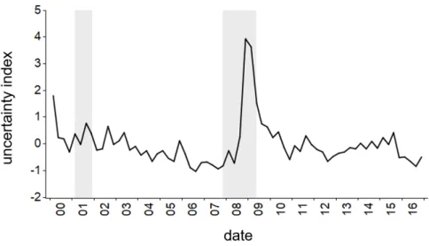
Ac-cordingly, uncertainty is measured from 2000Q1 to 2016Q4. Figure 1 shows the index of global short-run macroeconomic uncertainty (GSRMU). The index peaks around the Lehman Brothers collapse in 2008Q4, when the average uncertainty on world macro variables rises
to 4 standard deviations above its mean. It then drops during 2009 and 2010, and exhibits
only minor peaks afterwards. Figure 2 plots the index of global long-run macroeconomic uncertainty (GLRMU). The index surges during the Great Recession of 2008-2009, decreases
in 2010, then rises again in 2011 and gradually subsides afterwards.
The two figures show some similarities, stemming from the fact that the indices are
af-fected by the same shocks (the residuals used to generate the bootstrap samples for equations
12and13are the same). In particular, at the height of the global financial crisis, large shocks lead to increases in both short-run and long-run uncertainty. On the other hand, the indices
also exhibit remarkable differences, reflecting their different nature. The GSRMU index
con-cerns short-run fluctuations and the dynamic adjustment towards the long-run equilibrium.
Since it is conditional on the long-run parameters, it is a constrained measure of uncertainty
and is estimated using stationary time series (the first differences of I(1) variables and the
error correction terms). In late 2009 and 2010, when these variables typically return to
nor-mal after experiencing large deviations from their historical averages, short-run uncertainty
quickly reverts to lower values. Conversely, the GLRMU index is an unconstrained measure
of uncertainty and is effectively measured on non-stationary time series. As the shocks real-ized during and after the global crisis had permanent effects on the levels of the variables,
increases in long-run uncertainty persist after short-run uncertainty abates. As the figures show, short-run uncertainty rises more sharply than long-run uncertainty, in standardized
terms, during the global crisis.
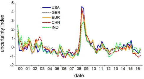
Figures 5 and 6 plot the country-level indices of short-run macroeconomic uncertainty (SRMU) and long-run uncertainty (LRMU), respectively, for a selection of advanced and
emerging economies: the U.S., the Euro area, the U.K., China and India. As is evident from
the graphs, country-specific measures are highly correlated. The average correlation across
all countries in the GVAR is 0.84 for SRMU and 0.82 for LRMU.14Such co-movement results
both from global uncertainty shocks, as captured by common factors in the GVAR residuals,
and from the dynamic propagation of uncertainty from one country to the others. The results
indicate that the estimated macroeconomic uncertainty is largely shared across countries.
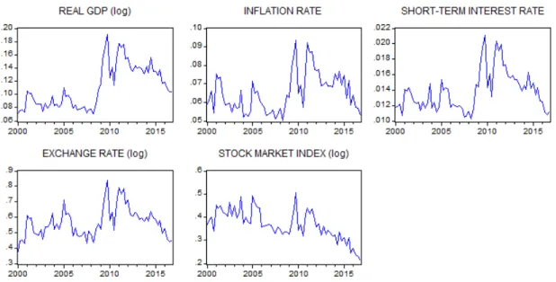
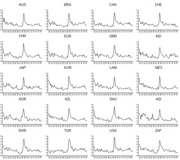
Figures 3 and 4 plot the global uncertainty measures (short-run and long-run, respec-tively) for each variable, i.e., the cross-country GDP-weighted averages of variable-specific
uncertainty. In this case the measures are not standardized, since uncertainty is not
aggre-gated across different types of variables. As the figures show, the time profiles of uncertainty
have strong commonalities, the main exception being a downward trend in stock market
uncertainty. Moreover, in absolute terms long-run uncertainty is systematically higher than
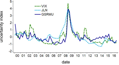
short-run uncertainty, due to the additional variability of cointegrating relationships. Next, the short- and long-run uncertainty indices are related to popular measures of
uncertainty. Figure 7 compares the GSRMU index with the VIX, i.e., the index of option-implied volatility in the S&P500, and with the U.S. macro uncertainty index developed by
Jurado et al. (2015) (JLN henceforth). All three measures peak in 2008Q4 and the size of their increase during the financial crisis is highly comparable, as well as the subsequent
de-cline in the period 2009-2010. Hence, short-run macroeconomic uncertainty appears broadly
consistent with expectations on financial market volatility over short horizons (the VIX
mea-sures 30-day-ahead risk-neutral expected volatility) and with uncertainty measured using
factor models with stochastic volatility, such as the JLN index (interestingly, the latter is constructed using stationary time series, which is in line with a short-run perspective focusing
on cyclical fluctuations rather than trends).
Barrero et al.(2016) find that economic policy uncertainty is more tightly linked to long-run than to short-long-run components of uncertainty. Figure 8 contrasts the GLRMU index with the news-based global EPU (GEPU) index developed by Baker, Bloom and Davis (see
Baker et al. 2016;Davis 2016). Unlike the indicators in Figure7, both GLRMU and GEPU exhibit relatively high values in the period 2010-2013, compared to their respective pre-crisis
averages. Only in 2016 they diverge substantially. Interestingly, however, this is not the
case when U.S.-specific measures are considered: figure 9 shows that the U.S. LRMU and EPU indices are very close in 2016 as well.15 While the results do not imply a systematic
relationship between the GLRMU and GEPU indices, uncertainty about the long run has
been arguably relevant for a variety of key policy issues debated in the aftermath of the
global financial crisis, such as financial regulation and Euro area reforms.
Table 1 shows the correlations between the different uncertainty measures considered, over the period 2000Q1-2016Q4. The GSRMU index is especially correlated with the VIX
(0.8) and JLN (0.66), while it has a lower correlation (0.21) with the GEPU index. On the
contrary, GLRMU is uncorrelated with the VIX and is negatively correlated with JLN (-0.15), while its correlation with the GEPU index is 0.35. Table2 reports the correlations between uncertainty measures for the United States only. In this case, the correlation between LRMU
and overall EPU rises to 0.59. Interestingly, the correlation between LRMU and the
news-based component of EPU (EPUn) is 0.31, suggesting that the divergence between the GEPU
index and GLRMU in 2016 (as shown in Figure8) may be in part explained by the exclusive reliance of GEPU on newspaper articles.
15The index considered here is the overall U.S. EPU index, which combines the news-based EPU index with
three additional measures of policy uncertainty: an index of tax expirations, a measure of forecast disagreement over consumer prices and a measure of forecast disagreement over federal/state/local government purchases. Both the U.S. EPU and the GEPU indices are available at www.policyuncertainty.com.
To conclude, the VIX and EPU indices are primary benchmarks for the two global un-certainty measures developed in this paper. While many events that trigger increases in
economic policy uncertainty also have repercussions on stock market volatility,16 the
differ-ent behavior of the two indices is well established and has already been ascribed by previous
research to a number of factors, including their different scope and horizon (Baker et al. 2016),17the existence of positive demand shocks offsetting the negative impact of policy
un-certainty on financial markets (ECB 2017), and the increased imprecision of political signals in recent years (Pastor and Veronesi 2017). The results presented in this paper are consistent with the idea that the VIX reflects a stronger focus on short-run economic issues, while policy
uncertainty is more related to the long-run consequences of economic shocks, at least in the
period under consideration (cf. Barrero et al. 2016).
3.2.2 Global spillovers of uncertainty
In this paragraph we study the cross-country spillovers of macroeconomic uncertainty using
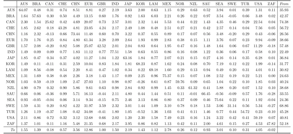
the methodology described in Section 2.3. Tables 3and 4 report all cross-country spillovers estimated on the full sample 1979Q1-2016Q4.18 Each number in the tables represents the
16This has been the case, for instance, with the Lehman Brothers default and the Troubled Asset Relief
Program (TARP) in 2008, or the Euro sovereign debt crisis in 2011.
17In particular, as argued byBaker et al.(2016): (i) the VIX has a short horizon, while the news-based
component of EPU has no specific horizon; (ii) policy issues do not necessarily relate to equity returns; (iii) the VIX covers publicly traded firms only. In addition, it has been pointed out that stock market-listed firms may focus excessively on short-term outcomes (a phenomenon known as short-termism, seeDavies et al. 2014;
Asker et al. 2015), which contrasts with the long-term focus of many policy issues (Barrero et al. 2016).
18The estimated spillovers from all countries to a given country do not exactly sum to 1, both because
they are obtained by bootstrap approximations and because the forecast variance decomposition is based on a linear approximation of a nonlinear function, as described in footnote11. However, the discrepancy is in general small. The sum of spillovers of short-run uncertainty is 0.97 on average and ranges between 0.91 and 1.01 across countries. The sum of spillovers of long-run uncertainty is 1.05 on average and ranges between 0.95 and 1.09. In the results reported in the paper, all spillovers are rescaled so that they exactly sum to 1 for each uncertainty-importing country.
contribution of the country in the column to the domestic uncertainty of the country in the row, in percentage. On average, uncertainty of foreign (non-domestic) origin accounts for
41% of domestic short-run uncertainty and 56% of long-run uncertainty.
The economies that generate the highest global spillovers are the Euro Area, the U.S.,
China and South-East Asia. Spillovers from the Euro Area are especially high in Turkey
(34% of short-run uncertainty and 24% of long-run uncertainty), Sweden (32% and 25%),
Norway (27% and 23%) and the U.K. (25% and 21%). The highest spillovers from the U.S.
are observed in Canada (23% and 14%), the Euro Area (10% and 6%), the U.K. (11% and
6%) and Mexico (5% and 8%). The Euro Area is a greater source of uncertainty for the U.S.
than the U.S. is for the Euro Area, especially in the long run: the spillovers from the Euro
Area to the U.S. are 13% of SRMU and 16% of LRMU, while the spillovers from the U.S.
to the Euro Area are 10% and 6%, respectively. As for spillovers from China, the rankings
differ between short-run and long-run uncertainty. More importantly, unlike the spillovers
from the Euro Area and the U.S., which tend to be higher for SRMU than LRMU, spillovers
of Chinese uncertainty are much stronger in the case of long-run uncertainty: the average
spillover from China, weighted by the PPP GDP of the destination countries in 2016, is about
4% of short-run uncertainty and 20% of long-run uncertainty (25% in the U.S. and 20% in
the Euro Area), indicating the pivotal role of China in the long-run outlook for the global economy. The Euro Area generates an average (PPP GDP-weighted) spillover of almost 13%
for SRMU and 12% for LRMU. The average U.S. spillover is about 4% for both SRMU and
LRMU. Finally, spillovers from South-East Asia are comparatively high in countries of the
Pacific region, such as New Zealand, Korea, Japan, Australia and Canada. The average
spillover accounts for 3% of other countries’ SRMU and 6% of LRMU.
The countries that receive the highest spillovers from the rest of world are Canada (where
the total foreign contribution is 74% of short-run uncertainty and 88% of long-run
uncer-tainty), Sweden (69% and 84%) and Switzerland (57% and 74%). Conversely, the countries
the total foreign contribution is 22%), South-East Asia (24%) and Mexico (25%), while for LRMU the countries with the lowest percent foreign contributions are China (25%), the
Latin American area (35%) and South-East Asia (36%).
Interestingly, our estimates of the average spillover effects are approximately halfway
be-tween those found byKlößner and Sekkel(2014), on the one hand, andRossi and Sekhposyan
(2017), on the other, both using a network approach. Klößner and Sekkel (2014) investigate spillovers of the EPU index between Canada, France, Germany, Italy, the U.K. and the U.S.
between 1997 and 2013. According to their estimates, the overall spillovers among these
counties account for approximately one quarter of total uncertainty. Rossi and Sekhposyan
(2017) study spillovers effects of output growth and inflation uncertainty within the Euro Area. They find that overall spillovers amount to about 74% of output growth uncertainty
and 78% of inflation uncertainty.
4 Conclusions
In an interconnected world economy, economic uncertainty is a global phenomenon. On the one hand, global uncertainty shocks hit different economies at the same time. On the other,
country-specific shocks spread across borders and increase uncertainty on a global scale.
This paper measures global macroeconomic uncertainty and investigates the cross-country
transmission of uncertainty using a GVAR model.
We construct two quarterly global indices: a global short-run macroeconomic uncertainty
(GSRMU) index, which measures the uncertainty on the short-run dynamics of the world
economy, and a global long-run macroeconomic uncertainty (GLRMU) index, which captures
the uncertainty on the long-run equilibrium. The indices are comprehensive, as uncertainty
is measured using both real and financial variables in a large network of countries. Moreover,
they can be constructed in real time and make minimal use of theoretical assumptions.
of Lehman Brothers, at the height of the 2007-2009 global financial crisis, and remains at relatively low levels from 2010 onwards, while the increase in GLRMU, first triggered by the
crisis, persists in its aftermath. The results may help explain the puzzle of the decoupling
between market volatility and policy uncertainty. A comparison of the two global indices with
the popular VIX and EPU indices suggests that over the last two decades financial market
volatility may have been closely associated with uncertainty on the short-run dynamics of
the economy, while policy uncertainty appears to have been more related to the long-run
consequences of the global financial crisis and the subsequent Euro area crisis.
Lastly, the paper quantifies global spillovers of macroeconomic uncertainty, which is a
novel contribution to the literature. The results highlight the importance of foreign sources
of domestic uncertainty, which explain 41% of country-specific SRMU and 56% of LRMU, on
average (with peaks of more than 70% in Canada, Switzerland and Sweden). The Euro Area
and the United States generate the highest global spillovers in terms of short-run uncertainty,
while China is the largest source of long-run uncertainty.
References
Ahir, H., N. Bloom, and D. Furceri, “World Uncertainty Index,” 2018. Unpublished. Asker, J., J. Farre-Mensa, and A. Ljungqvist, “Corporate Investment and Stock
Mar-ket Listing: A Puzzle?,” The Review of Financial Studies, 2015, 28 (2), 342–390.
Bachmann, R., S. Elstner, and E. Sims, “Uncertainty and Economic Activity: Evidence
from Business Survey Data,” American Economic Journal: Macroeconomics, 2013, 5 (2),
217–249.
Baker, S. R., N. Bloom, and S. Davis, “Measuring Economic Policy Uncertainty,” The Quarterly Journal of Economics, 2016, 131 (4), 1593–1636.
Barrero, J. M., N. Bloom, and I. Wright, “Short and Long Run Uncertainty,” 2016.
SIEPR Discussion Paper 16-030.
Berger, T., S. Grabert, and B. Kempa, “Global and Country-Specific Output Growth
Uncertainty and Macroeconomic Performance,” Oxford Bulletin of Economics and
Statis-tics, 2016, 78 (5), 694–716.
, , and , “Global macroeconomic uncertainty,” Journal of Macroeconomics, 2017, 53,
42–56.
Bernanke, B., “Federal Reserve Communications,” 2007. Speech at the Cato Institute 25th
Annual Monetary Conference, Washington, November 14.
Bloom, N., “The Impact of Uncertainty Shocks,” Econometrica, 2009, 77 (3), 623–685.
, “Fluctuations in Uncertainty,” The Journal of Economic Perspectives, 2014, 28 (2), 153–
175.
, M. Floetotto, N. Jaimovich, I. Saporta-Eksten, and S. Terry, “Really Uncertain
Business Cycles,” 2012. NBER Working Paper no. 18245.
Boswijk, H. P., G. Cavaliere, A. Rahbek, and A. M. R. Taylor, “Inference on
co-integration parameters in heteroskedastic vector autoregressions,” Journal of
Econo-metrics, 2016, 192 (1), 64–85.
Brainard, W., “Uncertainty and the Effectiveness of Policy,” American Economic Review,
1967, 57 (2), 411–425.
Carriero, A., T. E. Clark, and M. Marcellino, “Measuring Uncertainty and Its Impact
on the Economy,” 2017. Federal Reserve Bank of Cleveland Working Paper no. 16-22R.
, , and , “Assessing international commonality in macroeconomicuncertainty and its
Cavaliere, G., A. Rahbek, and A. M. R. Taylor, “Bootstrap Determination of the
Co‐Integration Rank in Vector Autoregressive Models,” Econometrics, 2012, 80 (4), 1721–
1740.
Cesa-Bianchi, A., M. H. Pesaran, and A. Rebucci, “Uncertainty and Economic
Ac-tivity: A Global Perspective,” 2014. CESifo Working Paper no. 4736.
Clements, M. P., “Assessing Macro Uncertainty In Real-Time When Data Are Subject To
Revision,” Journal of Business & Economic Statistics, 2017, 35 (3), 420–433.
Coibion, O. and Y. Gorodnichenko, “What Can Survey Forecasts Tell Us About
Infor-mational Rigidities?,” Journal of Political Economy, 2012, 120 (1), 116–159.
Collin-Dufresne, P., M. Johannes, and L. A. Lochstoer, “Parameter Learning in
General Equilibrium: The Asset Pricing Implications,” American Economic Review, 2016,
106 (3), 664–698.
Cuaresma, J. Crespo, F. Huber, and L. Onorante, “The macroeconomic effects of
international uncertainty,” 2019. ECB Working Paper No. 2302.
Davies, R., A. G. Haldane, M. Nielsen, and S. Pezzini, “Measuring the Costs of
Short-Termism,” Journal of Financial Stability, 2014, 12, 16–25.
Davis, S. J., “An Index of Global Economic Policy Uncertainty,” 2016. NBER Working
Paper No. 22740.
Dées, S., F. di Mauro, M. H. Pesaran, and L. V. Smith, “Exploring the International
Linkages of the Euro Area: a Global VAR Analysis,” Journal of Applied Econometrics,
2007, 22 (1), 1–38.
, S. Holly, M. H. Pesaran, and L. V. Smith, “Long Run Macroeconomic Relations in
the Global Economy,” Economics - The Open-Access, Open-Assessment E-Journal, 2007,
ECB, “Uncertainty and the Economic Prospects for the Euro Area,” Monthly Bulletin,
August 2009, pp. 58–61.
, “The Impact of Uncertainty on Activity in the Euro Area,” Economic Bulletin, 2016, 8,
55–74.
, “Assessing the Decoupling of Economic Policy Uncertainty and Financial Conditions,”
Financial Stability Review, May 2017, pp. 135–143.
Engle, R. F., “Long-Term Skewness and Systemic Risk,” Journal of Financial Econometrics,
2011, 9 (3), 437–468.
Forbes, K., “Uncertainty about uncertainty,” 2016. Speech at J.P. Morgan Cazenove “Best
of British” Conference, London, 23 November.
Gürkaynak, R., B. Sack, and E. Swanson, “The Sensitivity of Long-term Interest Rates
to Economic News: Evidence and Implications for Macroeconomic Models,” American
Economic Review, 2005, 95 (1), 425–36.
Hansen, L. P., “Beliefs, Doubts and Learning: Valuing Economic Risk,” American Eco-nomic Review: Papers & Proceedings, 2007, 97 (2), 1––30.
Hoffman, D. L. and R. H. Rasche, “Assessing Forecast Performance in a Cointegrated
System,” Journal of Applied Econometrics, 1996, 11 (5), 495––517.
IMF, “World Economic Outlook: Coping with High Debt and Sluggish Growth,” October
2012.
Johansen, S., Likelihood-Based Inference in Cointegrated Vector Autoregressive Models,
Oxford University Press, Oxford, 1995.
Jurado, K., S. C. Ludvigson, and S. Ng, “Measuring Uncertainty,” The American Economic Review, 2015, 105 (3), 1177–1216.
Klößner, S. and R. Sekkel, “International Spillovers of Policy Uncertainty,” Economic Letters, 2014, 124 (3), 508––512.
Lahiri, K. and X. S. Sheng, “Measuring Forecast Uncertainty by Disagreement: The
Missing Link,” Journal of Applied Econometrics, 2010, 25 (4), 514–38.
Lin, J. L. and R. S. Tsay, “Co-integration Constraint and Forecasting: an Empirical
Examination,” Journal of Applied Econometrics, 1996, 11 (5), 519–538.
Mohaddes, K. and M. Raissi, “Compilation, Revision and Updating of the Global VAR
(GVAR) Database, 1979Q2-2016Q4,” 2018. University of Cambridge, Faculty of Economics
(mimeo).
Mumtaz, H. and A. Musso, “The Evolving Impact of Global, Region-Specific, and
Country-Specific Uncertainty,” Journal of Business & Economic Statistics, 2019.
and K. Theodoridis, “Common and Country Specific Economic Uncertainty,” Journal of International Economics, 2017, 105, 205–216.
Orlik, A. and L. Veldkamp, “Understanding Uncertainty Shocks and the Role of Black
Swans,” 2014. NBER Working Paper no. 20445.
Orphanides, A. and J. C. Williams, “Inflation Scares and Forecast-Based Monetary
Policy,” Review of Economic Dynamics, 2005, 8 (2), 498–527.
and S. van Norden, “The Unreliability of Output-Gap Estimates in Real Time,” Review of Economics and Statistics, 2002, 84 (4), 569–583.
Ozturk, E. O. and X. S. Sheng, “Measuring Global and Country-Specific Uncertainty,” Journal of International Money and Finance, 2018, 88, 276–295.
Pastor, L. and P. Veronesi, “Explaining the puzzle of high policy uncertainty and low