ICT “bottlenecks” and the wealth of nations: a contribution to the empirics of economic growth
by
Leonardo Becchetti and Fabrizio Adriani 1. Introduction
The empirical literature on the determinants of economic growth has progressively tested the significance of factors which were expected to contribute to growth in addition to the traditional labour and capital inputs. In this framework valuable contributions have assessed, among others, 1 the role of: human capital (Mankiw-Romer-Weil, 1992) (from now on MRW), the government sector (Hall-Jones, 1997), social and political stability (Alesina-Perotti, 1994), corruption (Mauro, 1995), social capital (Knack-Keefer, 1997), financial institutions (Pagano, 1992; King-Levine, 1993) and income inequality (Persson-Tabellini, 1994; Perotti, 1996).
The paradox of this literature, though, is that it has left the labour augmenting factor of the aggregate production function unspecified. The impact of technological progress on the differences between rich and poor countries has therefore been neglected by implictly assuming that knowledge and its incorporation into productive technology is a public good, freely available to individuals in all countries (Temple, 1999).
This approach does not consider properly the nature of ICT and its role on growth. It neglects the fact that the core of ICT is made by weightless, expansible and infinitely reproducible knowledge products (software, databases) which create value in themselves, by increasing productivity of labour or by adding
1
Durlauf and Quah (1988) survey the empirical literature on growth and list something like 87 different proxies adopted to test the significance of additional factors in standard growth models. None of them is even akin to proxies adopted in this paper to measure factors crucially affecting ICT diffusion.
value to traditional physical products or traditional services. Knowledge products are almost public goods. Expansibility and infinite reproducibility make then nonrivalrous, and copyright (instead of patent) protection make them much less excludable than other type of innovation such as new drugs (Quah, 1999). If ICT would consist only of knowledge products, it should therefore be almost immediately available everywhere no matter the country in which it has been created. This does not occur though as the immediate diffusion and availability of knowledge products is prevented by some “bottlenecks”. In our opinion these “bottlenecks” are: i) the capacity of the network to carry the largest amount of knowledge products in the shortest time, ii) the access of individuals to the network in which knowledge products are immaterially transported and iii) the power and availability of terminals which process, implement and exchange knowledge products which flow through the network.
In this framework, economic freedom and the development of financial markets may affect both ICT diffusion and its impact on growth. Insufficient access provision and excess taxation limit the diffusion of personal computers and internet accesses (Quah, 1999). Liberalisation in the telecommunication sector reduces the costs of accessing the network and well developed financial markets make it easier to finance projects which aim to implement the capacity of the network and the quality of “terminals”.2
2
The relationship between information and communication technology and productivity has long been debated over the past three decades. In the 1980s and in the early 1990s, empirical research generally did not find relevant productivity improvements associated with ICT investments (Bender, 1986; Lovemann, 1988; Roach, 1989; Strassmann, 1990). This research showed that there was no statistically significant, or even measurable, association between ICT investments and productivity at any level of analysis chosen.
More recently, as new data were made available and new methodologies were applied, empirical investigations have found evidence that ICT is associated with improvements in productivity, in intermediate measures and in economic growth (Oliner and Sichel, 1994; Brynjolfsson and Hitt, 1996; Sichel, 1997; Lehr-Licthemberg, 1999).
The omitted consideration of “bottlenecks” reducing Information and Communication Technology (from now on BR-ICT), is partially justified so far by the scarcity of data,3 but has relevant consequences on the accuracy of growth estimates if this variable proves to be significant. First (omitted variable critique), if BR-ICT variables proxy for the level of technology are significant and omitted, parameters of the other MRW regressors (labour and investment in physical and human capital) are biased as far as they are correlated with it. Second (cross-sectional constant critique), the omitted specification of the labour augmenting technological progress biases regressions on the determinants of levels of per capita income as the difference in technological progress across countries cannot be treated as a cross-sectional constant, implicitly attributing the same level of technology to every observation (Islam, 1995; Temple, 1999).4 The solution of fixed effect panel data (Islam, 1995) is a partial remedy to it as it takes into account unobservable individual country effects.
In addition to reducing most of these problems, the inclusion of BR-ICT variables in the estimate may also avoid that uncontrolled heterogeneity in levels of per capita income lead to a significant correlation between the lagged level of per capita income and the error term in the convergence regressions thereby violating one of the required assumptions for consistency of OLS estimates (cross-country heterogeneity critique).5
In this paper we show that the introduction of BR-ICT variables, by allowing us to model the unknown country differences in the diffusion of technology, generates a sharp increase in the explanatory power of cross-sectional estimates of
3
Quah writes in 1999 that “the latest technologies have not been around for very long. Thus, convincing empirical time-series evidence on their impact will be difficult to obtain"”
4
The only relevant exception may be when regressions are run on regions with a certain degree of technological homogeneity such as the US states in the Barro-Sala-i-Martin (1992) paper on convergence.
5
According to Evans (1997) this problem can be neglected only when at least 90-95 percent of heterogeneity is accounted for.
the determinants of levels of income per worker and significantly reduces the effects of the cross-sectional constant and omitted variable critiques. The increased significance in the GDP per worker level regression reduces in turn the effects of the cross-country heterogeneity critique making it possible a cross-sectional estimate of convergence in growth rates.
The robustness of the main result of the paper (significance of the initial level and the rate of growth of BR-ICT technology in the cross-section and growth regressions) is accurately tested. With boostrap estimates we find that it is not affected by departures from the normality assumption for the distribution of the dependent variable. A sensitivity analysis which follows the Levine-Renelt (1992) approach shows that the introduction of measures of macroeconomic policy performance and of economic, civil and political freedom does not substantially weaken the significance of BR-ICT variables. Generalised 2-Stage Least Squares (G2SLS) panel estimates evidence that the ICT-growth relationship is not affected by endogeneity and exogenous subsample splits demonstrate that our evidence is robust to the issue of parameters heterogeneity.
The paper documents all these findings and is divided into four sections (including introduction and conclusions). In the second section we outline our theoretical hypotheses on the role of BR-ICT variables on aggregate growth. In the third section we present and comment empirical tests on our hypotheses.
2.1 The determinants of differences in levels of per capita growth The considerations developed in the introduction on the role of ICT on growth lead us to formulate the following hypothesis: Hypothesis 1: factors affecting ICT “bottlenecks” are a good proxy for measuring the amount technological progress which effectively augments labour productivity in a MRW human capital growth model
Consider the standard MRW (1992) production function taking into account the role of human capital:
Yt =F(K, H, AL) = α β
(
)
−α−β 1 t t t H AL K with α +β < 1 (1) where H is the stock of human capital, while L and K are the two traditional labour and physical capital inputs.Physical capital and human capital follow standard laws of motion.
(
K
AL
)
K
F
s
K
Y
s
K
K Kδ
δ
−
=
−
=
,
&
(2)(
K
AL
)
H
F
s
H
Y
s
H
H Hδ
δ
−
=
−
=
,
&
(3)where sk and sh are the fractions of income respectively invested
in physical and human capital.
The growth of the labour input is expressed as:
Lt = L0 e nt
. (4)
While in the standard MRW (1992) approach labour augmenting technological progress is exogenous, we make it explicit by assuming that most of it is proxied by weightless, infinitely reproducible, knowledge products (software,databases) which are conveyed to labour through crucial “bottlenecks” represented by the access to the network, the capacity of the network and the availability of “terminals” which process and exchange knowledge products.
We accordingly specify its dynamics as:
A(t) = AKP(t)ABR-ICT(t) (5)
with ABR-ICT(t) = ABR-ICT(0) e gBR-ICT(t)
and AKP(t) = AKP(0) e gKP(t)
ABR-ICT is a measure of the stock of ICT factors reducing the above
mentioned “bottlenecks” and gBR-ICT its rate of growth, while
weightless infinitely reproducible knowledge products and gKP is
its rate of growth.
We may therefore rewrite the production function in terms of output per efficiency units as y=k?h?.
From the model we can obtain the two standard growth equations:
(
)
t t k ts
y
n
g
k
k
&
=
−
+
+
δ
(6)(
)
t t h ts
y
n
g
h
h
&
=
−
+
+
δ
(7) where g=gBR-ICT+gKP .If we set the growth of physical and human capital equal to zero in the steady state we get:
β α β β
δ
− − −
+
+
⋅
=
1 1 1*
g
n
s
s
k
k h (8) β α α αδ
− − −
+
+
⋅
=
1 1 1*
g
n
s
s
h
k h . (9)Substituting h* and k* into the production function and taking logs we obtain:
(
)
= = ⋅ = − − α β β α * * * * * *,h Ak h A (0)e A (0)e k h k Af L Y g t ICT BR t g KP K P BR ICT (10) and:(
)
( )
( )
(
δ)
β α β α β α β β α α + + − − + − + − − + − − + + + = − − g n s s t g A c L Y h k ICT BR ICT BR t t ln 1 ln 1 ln 1 ln ln (0) (10’) or(
)
[
( ) (
)
]
( ) (
)
[
δ]
β α β δ β α α + + − − − + + + + − − − + + + = − − g n s g n s t g A c L Y h k ICT BR ICT BR t t ln ln 1 ln ln 1 ln ln (0) (10’’)where c=ln(AKP(0))+gKPtis the quasi-public good component of
countries.The difference with the traditional MRW (1992) specification is that we reinterpret the intercept and we add to it two additional terms measuring respectively the log of the stock of BR-ICT at the initial period and its rate of growth per time units. Therefore, the possibility that all countries have the same steady state level of per capita income depends not only on the levelling of their rate of population growth and of their physical and human capital investment rates, but also on their initial stocks and on their rates of growth of BR-ICT. The model therefore introduces an additional factor of conditionality for convergence in levels. A second important difference in this equation is that the country specific rate of growth of technology plus depreciation (g+δ in all previous models) is no more treated as fixed and equal to 0.05 for all countries6 (an heroic assumption) but it varies and is crucially influenced by the measured country specific growth rates of BR-ICT technology.
2.2 The determinants of differences in convergence of per capita growth
Under hypothesis 1 it is possible to show that, in the proximity of the balanced growth path, y converges to y* at the rate
(1-α-β (n+g)≡λ since the solution of the differential equation 7
dln(y)/dt=-λ[ln(y)-ln(y*)] (11)
is :
ln(yt)-ln(y*)=e-λt[ln(y0)-ln(y*)]. (12)
If we add ln(y*)- ln(y0) to both sides we get an equation
explaining the rate of growth:
6
This is the approach followed by Solow (1956), Mankiw-Romer-Weil (1992) and Islam (1995) among many others.
7
This obviously implies that the speed of convergence differs across countries and is crucially influenced by the pace of BR-ICT growth.
ln(yt)- ln(y0)=-(1-e -λt
)[ln(y0)-ln(y*)].
Replacing ln(y*) with our solution we get:
( )
( )
(
)
( )
0 0 ln ) 1 ( ln 1 ) 1 ( ln 1 ) 1 ( ln 1 ) 1 ( ) ln( ) ln( y e g n e s e s e y y t t h t k t t λ λ λ λ δ β α β α β α β β α α − − − − − − + + − − + − − + − − − + − − − = − (13) or: ( ) ( ) ( ) (1 )ln(( / )(0)) (1 )ln( ) ln 1 ) 1 ( ln 1 ) 1 ( ln 1 ) 1 ( ' )) 0 )( / ln(( ) )( / ln(( ) 0 ( ICT BR t t t h t k t ICT BR A e L Y e g n e s e s e t g c L Y t L Y − − − − − − − − + − − + + − − + − − + − − − + − − − + + = − λ λ λ λ λ δ β α β α β α β β α α (13’) where ' (1 t)ln( KP(0)) KPt e A g c = + − −λ .The difference with respect to the traditional MRW approach is in the interpretation of the common intercept (which incorporate to us the worldwide diffusion of quasi-public knowledge products) and in the fact that convergence may be prevented by differences in the stock of initial BR-ICT factors or in their rates of growth.
3.1 Empirical analysis: the database and descriptive statistics
Variables for our empirical analysis are taken from the World Bank database.8 The dependent variable Y/L is the gross domestic product per working-age person converted to international dollars using purchasing power parity rates,9 L is
8
We cannot use the Penn World Tables as the time period for which we dispose of BR-ICT data does not significantly overlap with that of the Summers-Heston database.
9
An international dollar has the same purchasing power over GDP as the U.S. dollar in the United States.
number of people who could potentially be economically active (population aged between 15-64). sk is gross domestic investment
over GDP, sh is the (secondary education) ratio of total
enrollment, regardless of age, to the population of the age group that officially corresponds to the level of education shown (generally the 14-18 age cohort).10 To measure factors reducing ICT bottlenecks we consider four different proxies: i) the number of main telephone lines per 1,000 inhabitants;11 ii) internet hosts (per 10,000 people) or the number of computers with active Internet Protocol (IP) addresses connected to the Internet, per 10,000 people; iii) mobile phones (per 1,000 people); iv) personal computers (per 1,000 people).12
Tab. 1 provides some descriptive statistics on the above mentioned variables and shows that the dependent variable is not normally distributed when we both consider individual year and overall sample datasets. This fact, neglected by the existing literature, should be taken into account when running regressions in levels and rates of growth. Furthermore, simple statistics of sigma convergence clearly confirm that BR-ICT indicators are far from being a freely available public goods as the variability in the diffusion of BR-ICT across countries is extremely high and persistent (Fig. 1). On average for the entire observation period, it is higher when we consider the latest ICT innovation (the standard deviation of the diffusion of internet hosts across
10 It is also defined as gross enrollment ratio to compare it with the ratio (net
enrollment ratio) in which the denominator is the enrollment ratio only of the age cohort officially corresponding to the given level of education.
11
Telephone mainlines are telephone lines connecting a customer's equipment to the public switched telephone network. Data are presented per 1,000 people for the entire country.
12
Since all these factors are expected to ease the diffusion and processing of knowledge products in the internet a qualitative measure of their “power” (i.e. the processing capacity of PCs) would improve the accuracy of our proxies. Such information though is not available for long time periods and across the countries observed in oru sample.
countries is two and a half its mean while it is almost equal to its mean in the case of the diffusion of main telephone lines).
Tab A.1 in the Appendix gives the list of countries with sufficient observations which have been selected in the estimates with each of the four BR-ICT proxies. For each country we display the level of the BR-ICT variable in the first and in the last available year. This table documents that we have data for 115 countries from 1983 if we just consider the diffusion of telephone lines, while for much less countries and more limited time, if we consider the other three BR-ICT indicators.
For this reason we define a composed indicator which is an unweighted average of each of the four normalised BR-ICT indicators (when available). We then perform our estimates with the composed and with each of the individua l BR-ICT indicators.
3.2 Econometric estimates of the determinants of levels of income per worker
As a first step we regress equation (1) in levels.13 Our time span is quite limited when we consider a common starting year for individual BR-ICT indicators (1991-97), while it becomes much wider when we use the composite indicator. Tables 2 compares results from the standard MRW model with the model specified in (1) with the different BR-ICT indicators.14
13
We perform the estimate with four different specifications which alternatively consider the ILO labour force and population in working age as labour inputs and observed income or trend income as a dependent variable. The ILO labor force includes the armed forces, the unemployed, and first-time job-seekers, but excludes homemakers and other unpaid caregivers and workers in the informal sector. We use trend income alternatively to observed income to avoid that our results be influenced by cyclical effects on output (Temple, 1999). Estimates with the alternative proxies for the labour input and the dependent variable do not differ substantially and are available from the authors upon request.
14
By estimating (10’’) we implicitly impose the restriction of equality between the coefficient of log(n+g+δ) and the sum of coefficients of logs of sk and sh
A first think to be noted is that elasticities of investment in physical and human capital are, as expected, much smaller on such a limited time span (1991-97) also in the traditional MRW estimate, even though both factors significantly affect levels of income per worker. The introduction of starting year le vels (A
BR-ICT(0)) and rates of growth of BR-ICT variables (gBR-ICT)
significantly improves the overall goodness of fit and explains almost 94 percent of the cross-sectional heterogeneity in the specification in which BR-ICT is proxied by the diffusion of personal computers. ABR-ICT(0) and gBR-ICT variables are always
strongly significant and with the expected sign. On the other hand, the fact that their slopes are smaller than one, the value implicitly assumed by the econometric specification, supports the intuition that ICT is bottleneck reducing. In fact, roughly speaking, one can think of the coefficients of these two variables15 as the returns of BR-ICT in spreading knowledge. It is, therefore, rather intuitive that widening a bottleneck has decreasing returns as it progressively reduces pressure. The strong significance of the constant term also confirms the hypothesis that BR-ICT factors do not exhaust the contribution of technology to growth and that a common (quasi) public technological factor exists to which (in our opinion) knowledge products contribute. While for the second variable an instrumental variable test is needed to check whether our results are affected by endogeneity (see the generalised 2-stage least square specification explained further), this is certainly not the case for the lagged BR-ICT level (A BR-ICT(0)).
Furthermore, the four regressors included in (10’’) are all significant only when we use the composite index, while in almost all other cases the introduction of the BR-ICT variables seems to cast doubts on the significance of the short term
15
Test on the equalituy of ABR-ICT and gBR-ICT coefficients in Tab 2 show that
consistently with our hypothesis these coefficients are not significantly different from each other and almost identical in the 1983-1997 sample (respectively 0.302 and 0.299).
elasticity of the investment in physical capital and also on that of human capital when we specify the BR-ICT variable with mobile phones or personal computers.16 The reestimation of the model with bootstrap standard errors shows that the significance of the BR-ICT variables remains strong for all considered indicators.
A final estimate done by using the composite index on the 1983-1997 time range gives us the idea of what happens when we extend the estimation period and when regression coefficients measure medium and not short term elasticities. Magnitudes of physical and human capital investment coefficients are now higher and closer to those found in MRW. A striking result is that sk is no more significant when BR-ICT is included in the
estimate, while sh is significant and the implied β is .23.
17 This number is below the range calculated by MRW for the US.18 The first result seems to suggest that, a part from the difference in estimation periods , the physical capital contribution falls when we properly consider the role of BR-ICT technological factors (which, in a late sense, are part of physical capital). In the same originary MRW (1992) estimate the physical capital factor share
and the coefficient of the log of (n+g+δ). Estimates in which the assumption is removed do not provide substantially different results and are available from the authors upon request.
16
The weakness of the human capital variable when we introduce personal comp uters is consistent with the hypothesis that the productive contribution of skilled workers passes through (or is enhanced by) the technological factor. For evidence on this point see Roach (1991), Berndt et al. (1992) and Stiroh (1998).
17
The lack of significance of sk can be anticipated even by the simple
inspection of descriptive statistics. If we divide our sample into three equal subgroups of countries according to levels of income per worker (high, medium and low income) we find that values of sh are
respectively 83.60, 58.92 and 50.46, while values of sk are much more
equal across subgroups (23.57, 23.18 and 23.00) 18
According to MRW which compare minimum wage to average manufacturing wage in the US, the human capital factor share should be between 1/2 and 1/3.
drops to 0.14 in the OECD sample from 0.41 in the overall sample and this change may be consistent with our results given the higher contribution of BR-ICT technology to output in the first group of countries.
Further support for this hypothesis comes from the Jorgenson-Stiroh (1999) empirical paper showing the dramatical decrease in the selling and rental price of computers in the USA, paralleled by an increase in the same prices for physical capital between 1990 and 1996. Since the decline in computer prices depends on liberalisation and competition on domestic ICT markets it is reasonable to assume that there has been much more substitution between BR-ICT and physical capital in the most advanced OECD countries and therefore that, cross country higher levels and growth rates of income per worker are associated with higher level and growth rates of BR-ICT diffusion, but not necessarily with higher rates of investment in physical capital.19
Output elasticities of the two BR-ICT variables, when included in our estimate seem therefore to reduce the output elasticity of human capital and to obscure the cross-sectional contribution of physical capital, but significantly contribute to explain large differences in income per capita which would remain partially unexplained would the role of BR-ICT technology be neglected. The reasonable interpretation for this finding is that part of the contribution of human capital to output
19
The same shift in technological patterns induced by the ICT revolution seems to be an autonomous cause of substitution between ICT and physical capital since ICT investment modifies the trade-off between scale and scope economies. The ICT literature finds that, while software investment increases the scale of firm operations, telecommunications investment creates a “flexibility option” easing the switch from a Fordist to a flexible network productive model (Milgrom-Roberts, 1988) in which products and processes are more frequently adapted to satisfy consumers' taste for variety (Brooke, 1991; Barua-Kriebel-Mukhopadhyay, 1991; Paganetto-Becchetti-Londono, 2000).
depends on BR-ICT technology.20 The former is overstated if the latter is not accounted for.
The use of a cross-sectional regression for estimating the determinants of levels of per capita income has been strongly criticised by Islam (1995). His argument is that, since the labour augmenting A-factor in the aggregate production function represents country specific preferences and technological factors, it is not possible to assume that it is absorbed in the intercept and is therefore constant across countries (cross-sectional constant critique). Our estimate overcomes the problem by specifying the technological variable but what if some additional country specific variables (deep fundamentals such as ethos or governance parameters such as economic freedom) are omitted ? We have two solutions here: i) a reestimation of (1) as a cross-section with the introduction of variables which may proxy for those omitted; ii) a panel estimate of the same equation in which fixed effects capture all additional country specific variables. 21
With respect to the first approach we propose a sensitivity analysis in which we subsequently introduce three by three combinations of the following additional explanatory variables: i) average government consumption to GDP; ii) export to GDP; iii) inflation; iv) standard deviation of inflation; v) average rate of government consumption expenditures; vi) average growth rate of domestic credit; vii) standard deviation of domestic credit and, finally, three indexes of economic, civil and legal freedom.22 All
20
It is reasonable to figure out, for instance that higher world processing capacity or the possibility of exchanging information in internet increases the productivity of high skilled more than that of low skilled workers.
21
The fixed effect is preferred to the random effect approach as the second retains the strong assumption of independence between regressors and the disturbance term.
22
The role of inflation on growth is examined, among others by Easterly and Rebelo (1998). For a survey on the role of financial variables on growth see Pagano (1993). The impact of political variables including political freedom
has been analysed by Brunetti (1997). The relationship between
economic freedom and growth has been investigated, among others, by Dawson (1998) and by Easton-Walker (1997)
these variables, with the exception of indexes of economic, civil and legal freedom are also used by Levine-Renelt (1992) in their sensitivity analysis on the determinants of growth.
Results of sensitivity analysis run on the 1985-1997 period with the BR-ICT composite index show that all regressors of specification (1) are substantially robust (no change in significance and limited change in magnitude) to the inclusion of any combination of the above mentioned additional explanatory variables (Table 3). 23
Since the sensitivity analysis emphasizes the strong significance of economic freedom we reestimate the model by adding this variable and by decomposing it into its seven attributes (Table 4). In this way we find that five of the seven attributes are significant (legal structure and property rights, structure of the economy and use of markets, freedom in financial markets, in foreign trade and in exchange markets) while only government size and macroeconomic stability do not directly affect growth in the cross-sectional estimate in levels.
With respect to the second approach suggested to overcome the cross-sectional constant critique, fixed effect panel results confirm the robustness of the significance of the technological variable (Table 5). The ICT significance in fixed effect panel estimates is also robust to the inclusion of any combination of additional regressors (Tab. 6a). Our results are a direct answer to Islam (1995) interpretation of country specific fixed effects in its MRW panel estimate which he finds significantly and positively correlated with growth rates and human capital and interpret as country specific technology effects. Since our BR-ICT variables are positive and significant and their inclusion reduces the impact of human capital they are formally (in definition) and substantially (in data) a relevant part of the fixed effects measured by Islam (1995).
23
The different estimation period with respect to Table 2 is necessary for the reduced availablity of data on civil, legal and economic freedom.
This type of estimate, though, generates an endogeneity problem since the contribution of BR-ICT is no more split into the two components of initial levels and rates of growth and is therefore not completely lagged with respect to the dependent variable.
To rule out endogeneity problems of estimates in levels we use the G2SLS methodology which combines fixed effect panel estimates with instrumental variables. We use as instruments two period to four period lagged values of BR-ICT indicators and find that BR-ICT variables are still significant (Tables 5-7b).
Results from Table 4 seemed to show that the governance of financial and trade markets was a fundamental factor for growth. The development of financial markets though may even have an impact on the relationship between BR-ICT and growth.24 Technological innovation and investment in technologies which may reduce ICT bottlenecks (optic fibers, power enhanced mobile phones) is in fact easier to implement in well developed capital markets where it can be equity financed since equity financiers are residual claimants of the expected increase in value generated by the innovation and find it instantaneously incorporated into their share prices. Furthermore, in well developed financial markets, the unobserved quality or power of BR-ICT innovation rate and ICT diffusion is therefore expected to be higher and our BR-ICT proxies (not corrected for quality) to have an increased significance on levels and growth of income per capita.
Exogenous subsample splits help us to investigate whether the BR-ICT - growth relationship is stronger, as we postulated, in countries with more developed financial markets. Consistently with our assumption we find that the significance of
24
Saint Paul (1992) finds a trade-off between technological diversification (which implies despecialisation and no choice of the more specialised
technology) and financial diversification. The development of financial markets allows entrepreneur to achieve diversification on financial market and therefore to reduce technological diversification by choosing the riskier and more profitable technology.
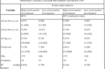
BR-ICT variables is much more pronounced in the OECD and in the higher economic freedom subsample than in their complementary samples (Tab. 7a). Since our index of economic freedom measures at most the development of the banking system (which may proxy but does not coincide with the development of equity markets), we propose an additional indicator based on the stock market capitalisation to GDP. Results from this indicator are consistent with those on the development of the banking system with the BR-ICT factor being more significantly related to income per worker in the high development subgroup in panel fixed effect estimates (Table 7c).
To check whether our results are affected by endogeneity we perform G2SLS panel estimates on these samples. Unfortunately the limited number of degrees of freedom available when we use lagged instruments allows us to estimate the model with sufficient confidence only for the financial freedom split and for the ICT1 and composed index indicators. In these specific cases G2SLS estimates show that, once endogeneity is taken into account, differences between countries with high and low economic freedom persists (tab. 7b).
3.3 Econometric estimates of convergence in rates of growth of income per worker
The reduced interval for which we dispose of ICT data limits our analysis to short-medium term convergence and prevents us to estimate convergence with panel data. Nonetheless, since the best specification of (10’’) explains almost 95 percent of the observed cross-sectional heterogeneity our attempt at estimating convergence with a cross-sectional estimate is not severely affected by the cross-country heterogeneity critique (Evans, 1997). The results we obtain are roughly in line with the existing literature and with our theoretical predictions formulated in section 2. Tab. 8 shows that our ICT-growth model performs better than the MRW model in the 90es. The level of income per
working-age person in the starting period (Y/L1985) becomes
significant only once we proxy the labour augmenting technological progress with our BR-ICT variables. This suggests that evidence of convergence in the short run can be found only when we consider its conditionality to investment not only in physical capital,25 but also in BR-ICT. If we arbitrary set (n+δ + g) equal to 0.05 for all countries our implied λ is larger than that in MRW and lower than in Solow (1956) and in Islam (1995). It is also slightly larger when we introduce BR-ICT variables. In interpreting our result of faster convergence we must consider that we are working on a reduced and almost non overlapped sample period with respect to MRW (1983-1997 against 1960-1985). In this period convergence looks faster when it is conditioned to variables relevant in our model.
Sensitivity analysis on this result finds that it is confirmed even when we use bootstrap standard errors (and we consider the composite BR-ICT index or the PC diffusion variable) and that it is robust to the inclusion of three by three combinations of all additional variables used in Levine-Renelt (1995) sensitivity analysis plus all different attributes of economic freedom (Tab. 9 and 10).
Conclusions
The technological revolution originated by the progressive convergence of software and telecommunications and fostered by the advancements in digital technology is dramatically changing the world. This revolution has sharply reduced transportation costs, deeply modified geographical patterns of
25 The lack of significance of the coefficient of human capital is a well known
result in the literature. Islam (1995) explains it arguing that the positive cross-sectional effect of human capital is likely to be outweighted by the negative temporal effect (higher levels of investment in human capital did not produce positive changes in growth). This is not the case for BR-ICT investment which are shown to have also positive temporal effects in our estimate.
productive factors across the world and significantly increased the productivity of human capital.
ICT mainly consists of a core of reproducible and implementable knowledge incorporated in quasi-public “knowledge products” such as software and database libraries which can be accessed by everyone at some conditions. These conditions are represented by capacity and access to the network and by the availability of efficient terminal nodes which allow to process, exchange and reproduce these knowledge products. The wealth of nations therefore crucially depends on the quality of telephone lines, on the number of personal computers, mobile phones and internet hosts as these factors reduce bottlenecks which may limit the diffusion of technological knowledge.
The empirical literature of growth has so far neglected this phenomenon for limits in the available information or under the theoretical assumption that technology is a public good which can be easily and costlessly incorporated into domestic aggregate production functions. Our empirical evidence demonstrates that this is not the case and finds - even though for a limited time span with respect to the traditional empirical analyses on growth - some interesting results which support the theoretical prediction of a significant role of BR-ICT in explaining levels and rates of growth of income per worker. Our results clearly show that the BR-ICT factor is an additional crucial factor of conditionality for convergence in levels and rates of growth and our finding is robust to changes in specification and in the estimation approach.
Table 11 resumes rationale s, critical issues and main results of our empirical approaches showing how we rationally moved from the simplest to more sophisticated approaches in order to provide answers to the most important critical issues raised in the empirical literature. Results obtained from the methodological path followed are satisfactory when we look at both level and convergence estimates whose robustness has been tested under several alternative methods.
We may therefore conclude that BR-ICT is another crucial variable which bridges the gap between pessimist views arguing that differences in personal income across countries are a structural element of the economic system which is going to persist and even widen, and optimist views believing that those who lag behind will be able to catch up.
By collecting additional information on ICT diffusion in the next years we will be able to know whether BR-ICT contribution to growth is likely to persist also in the future so that our conclusions may be extended to a longer time period.
References
Alesina, A., Perotti, R., 1994, The political economy of growth: a critical survey of the recent literature, World Bank Economic Review, 8:3, pp.351-71.
Barrol R., Sala -i-Martin, X., 1992, Convergence, Journal of Political Economy, 100, pp.223-251.
Barua, A., Kriebel, C. and Mukhopadhyay, T. [1991], "Information Technology and Business Value: An Analytic and Empirical Investigation," University of Texas at Austin Working
Paper, (May).
Berndt, Ernst R., Morrison, Catherine J. and Rosenblum, Larry S.,
[1992], "High-tech Capital Formation and Labor
Composition in U.S. Manufacturing Industries: an Exploratory Analysis," National Bureau of Economic Research Working Paper No. 4010, (March).
Becchetti, L., Londono Bedoya, D.A., Paganetto, L., 2000, ICT investment, productivity and efficiency: evidence at firm level using a stochastic frontier approach, CEIS Working paper n.126. Bender, D. H. [1986], Financial Impact of Information Processing. Vol. 3(2): 22-32.
Brunetti, A., 1997, Political varia bles in cross-country growth analysis, Journal of Economic Surveys, vol. 11. N.2, pp.162-190. Brynjolfsson. Erik and Hitt, Lorin. [1996], "Paradox Lost?
Firm-Level Evidence on the Returns to Information Systems
Spending", Management Science, (April)
Caselli, F., Esquivel, G., Lefort, F., 1996, Reopening the convergence debate; a new look at cross-country growth empirics, Journal of Economic Growth, 1:3, pp. 363-90
Dawson, J. W., Institutions, Investment, and Growth: New Cross-Country and Panel Data Evidence, Economic Inquiry; 36(4), October 1998, pages 603-19.
Durlauf, S.N., Quah D.T., 1998, The new empirics of economic growth, Center for Economic Performance Discussion Paper N. 384.
Easterly, W., Rebelo, S., 1993, Fiscal Policy and Economic growth, Journal of Monetary Economics, 32:3, pp.417-58.
Easton, S. T.; Walker, M. A., 1997, Income, Growth, and Economic Freedom, American Economic Review; 87(2), May 1997, pages 328-32.Knack, Stephen and Phillip Keefer (1997) "Does Social Capital Have an Economic Payoff? A Cross-Country Investigation" Quarterly Journal of Economics 112: 1251-88
Evans, P., 1997, How fast do economies converge ?, The Review of Economics and Statistics, pp.219-225
Gwartney, J.; R. Lawson and D. Samida (2000), “Economic Freedom of the World: 2000”, Vancouver, B.C., The Fraser Institute.
Islam, N., 1995, Growth empirics: a panel data approach, Quarterly Journal of Economics, pp.1127-1169.
Jorgenson, D., K.J. Stiroh , 1999, Information technology and growth, American Economic Review, Vol. 89, No. 2, pp. 109-115. King, R.G. Levine, R. (1992 ) "Finance and growth: Schumpeter
might be right", The Quarterly Journal of Economics, August. Lehr, B., Lichtenberg, F., 1999, Information Technology and Its
Impact on Productivity: Firm-Level Evidence from Government and Private Data Sources, 1977-1993, Canadian Journal of Economics; 32(2), pp. 335-62. Levine, R., Renelt, D., 1992, A sensitivity analysis of cross-country growth regressions, American Economic Review, 82(4), 942-63.
Loveman, Gary W. "An Assessment of the Productivity Impact of
Information Technologies," MIT Management in the
1990s, Working Paper # 88 – 05, July 1988.
Mankiw, N.G., Romer, D., Weil, D., 1992, A contribution to the empirics of economic growth, Quarterly Journal of economics, May, pp. 407-437.
Mauro, P., 1995, Corruption and growth, Quarterly Journal of Economics, 110:3, pp.681-712.
Milgrom P., Roberts R., (1988), The Economics of Modern Manufacturing: Products, Technology and Organization, Stanford Center for Economic Polic y Research Discussion Paper 136
Pagano, M. (1993) "Financial markets and growth: an overview", European Economic Review 37, pp. 613-622.
Persson, T., Tabellini, G., 1994, Is inequality harmful for growth?, American Economic Review, 84:3, pp. 600-21.
Perotti, R., 1996, Growth, income distribution and democracy: what the data say, Journal of Economic Growth , 1, pp.149-87. Roach, Stephen S. [1991], "Services under Siege: the Restructuring Imperative," Harvard Business Review 39(2): 82-92, (September-October).
Mankiw, N.G., Romer D., Weil, D.N., 1992, A contribution to the empirics of economic growth, Quarterly Journal of Economics, 107: 2, 407-37.
Oliner, Stephen D. and Sichel, Daniel E. [1994], "Computers and Output Growth Revisited: How Big is the Puzzle?" Brookings Papers on Economic Activity, 1994(2): 273-334.
Roach, Stephen S. [1989], "America's White-Collar Productivity Dilemma," Manufacturing Engineering , August , pp. 104. Sichel, Andrew. 1997. The Computer Revolution: An Economic Perspective. Brookings Institution Press, Washington, DC. Solow, R.M., 1956, A contribution to the theory of economic growth, Quarterly Journal of Economics, LXX, pp.65-94.
Stiroh, K.J., 1998, Computers productivity and input substitution, Economic Inquiry, 36,2, April, 175-91.
Strassmann, P. A. [1990], The Business Value of Computers: An
Executive's Guide. New Canaan, CT, Information
Economics Press.
Temple, J., 1999, The new growth evidence, Journal of Economic Literature, Vol. XXXVII, pp.112-156.
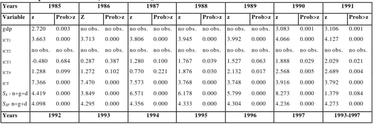
Tab. 1 Shapiro-Wilks normality tests on selected regressors
Years 1985 1986 1987 1988 1989 1990 1991
Variable z Prob>z Z Prob>z z Prob>z z Prob>z z Prob>z z Prob>z z Prob>z
gdp 2.720 0.003 no obs. no obs. no obs. no obs. no obs. no obs. no obs. no obs. 3.083 0.001 3.106 0.001 ICT1 3.663 0.000 3.713 0.000 3.806 0.000 3.945 0.000 3.992 0.000 4.066 0.000 4.127 0.000 ICT2 no obs. no obs. no obs. no obs. no obs. no obs. no obs. no obs. no obs. no obs. no obs. no obs. no obs. no obs. ICT3 -0.480 0.684 0.287 0.387 1.280 0.100 1.767 0.039 1.527 0.063 1.888 0.029 2.029 0.021 ICT4 1.288 0.099 1.272 0.102 0.770 0.221 1.876 0.030 2.132 0.017 2.568 0.005 2.689 0.004 ICT 7.366 0.000 7.470 0.000 7.573 0.000 3.768 0.000 3.748 0.000 3.916 0.000 3.792 0.000 Sk - n+g+d 4.419 0.000 3.849 0.000 6.571 0.000 6.178 0.000 5.799 0.000 8.273 0.000 1.379 0.084 SH- n+g+d 4.098 0.000 4.295 0.000 4.356 0.000 4.333 0.000 4.304 0.000 4.236 0.000 4.273 0.000 Years 1992 1993 1994 1995 1996 1997 1993-1997
Variable z Prob>z z Prob>z z Prob>z z Prob>z z Prob>z z Prob>z z Prob>z
gdp 2.988 0.001 3.119 0.001 2.957 0.002 2.974 0.001 3.064 0.001 2.864 0.002 11597 0.000
ICT1 4.163 0.000 4.151 0.000 4.228 0.000 4.337 0.000 4.450 0.000 4.485 0.000 7052.0 0.000 ICT2 no obs. no obs. no obs. no obs. 2.119 0.017 1.503 0.066 1.810 0.035 1.756 0.040 2119.0 0.017 ICT3 1.954 0.025 2.172 0.015 2.467 0.007 3.021 0.001 3.471 0.000 3.446 0.000 5063.0 0.000 ICT4 2.761 0.003 2.748 0.003 2.675 0.004 2.818 0.002 2.835 0.002 2.857 0.002 7426.0 0.000 ICT 3.632 0.000 3.524 0.000 3.346 0.000 3.418 0.000 3.466 0.000 3.469 0.000 6474.0 0.000
Sk - n+g+d 4.519 0.000 3.136 0.001 4.277 0.000 3.046 0.001 3.458 0.000 1.063 0.144 5243.0 0.000
SH- n+g+d 4.294 0.000 3.801 0.000 3.942 0.000 4.240 0.000 2.711 0.003 5.362 0.000 10233. 0.000
Note: ICT1: main telephone lines per 1.000 people; ICT2: internet hosts (or the number of computers with active Internet Protocol (IP) addresses connected to the Internet) per 10,000 people; ICT3: Mobile phones (per 1,000 people). ICT4: Personal computers (per 1,000 people); ICT (COMPOSITE INDEX): unweighted average of ICT1, ICT2, ICT3 and ICT4.
Fig. 1: Sigma convergence of BR-ICT indicators (standard deviation to mean ratios)
Note: sdICT1: standard deviation of main telephone lines per 1.000 people; sdICT2: standard deviation of internet hosts (or the number of computers with active Internet Protocol (IP) addresses connected to the internet) per 10,000 people; sdICT3: standard deviation of mobile phones (per 1,000 people). sdICT4: standard deviation of personal computers (per 1,000 people). The last symbol represents sdICT (COMPOSITE INDEX): unweighted average of ICT1, ICT2, ICT3 and ICT4.
Year sdICT1 sdICT2 sdICT3 sdICT4 1985 1986 1987 1988 1989 1990 1991 1992 1993 1994 1995 1996 1997 0 1 2 3
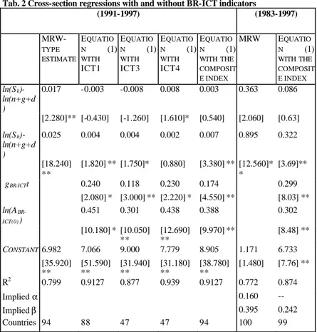
Tab. 2 Cross-section regressions with and without BR-ICT indicators (1991-1997) (1983-1997) MRW-TYPE ESTIMATE EQUATIO N (1) WITH ICT1 EQUATIO N (1) WITH ICT3 EQUATIO N (1) WITH ICT4 EQUATIO N (1) WITH THE COMPOSIT E INDEX MRW EQUATIO N (1) WITH THE COMPOSIT E INDEX ln(Sk )-ln(n+g+d ) 0.017 -0.003 -0.008 0.008 0.003 0.363 0.086 [2.280]** [-0.430] [-1.260] [1.610]* [0.540] [2.060] [0.63] ln(Sh )-ln(n+g+d ) 0.025 0.004 0.004 0.002 0.007 0.895 0.322 [18.240] ** [1.820] ** [1.750]* [0.880] [3.380] ** [12.560]* * [3.69]** gBR-ICTt 0.240 0.118 0.230 0.174 0.299 [2.080] * [3.000] ** [2.220] * [4.550] ** [8.03] ** ln(A BR-ICT(0) ) 0.451 0.301 0.438 0.388 0.302 [10.180] * [10.050] ** [12.690] ** [9.970] ** [8.48] ** CONSTANT 6.982 7.066 9.000 7.779 8.905 1.171 6.733 [35.920] ** [51.590] ** [31.940] ** [31.180] ** [38.780] ** [1.480] [7.76] ** R2 0.799 0.9127 0.877 0.939 0.9127 0.772 0.874 Implied α 0.160 -- Implied β 0.395 0.242 Countries 94 88 47 47 94 100 99
Note: the Table reports results on the estimation of equation (1). In the second to fourth column the traditional MRW approach is augmented with ICT variables. ICT1: main telephone lines per 1.000 people. ICT3: Mobile phones (per 1,000 people). ICT4: Personal computers (per 1,000 people); ICT COMPOSITE INDEX: unweighted average of ICT1, ICT2, ICT3 and ICT4 where ICT2 is the number of computers with active Internet Protocol (IP) addresses connected to the internet) per 10,000 people. g is gBR-ICT+gKP, where gBR-ICT is the
growth rate of the selected ICT variable, and gKP is assumed constant across countries. Sh ,
Sk and gBR-ICTt are calculated as estimation period averages, while the dependent variable
has the end of period value.T -stats are reported in square brackets. ** 95 percent significance with boostrap standard errors, * 90 percent significance with boostrap standard errors. We use the percentile and bias corrected approach with 2000 replications.
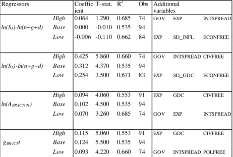
Tab. 3 Sensitivity analysis on cross-section regressions (1985-1997 estimates with the composite BR-ICT index)
Regressors Coeffic
ient
T-stat. R2 Obs Additional variables
High 0.064 1.290 0.685 74 GOV EXP INTSPREAD
ln(Sk)-ln(n+g+d) Base 0.000 -0.010 0.535 94
Low -0.006 -0.110 0.662 84 EXP SD_INFL ECONFREE
High 0.425 5.860 0.660 74 GOV INTSPREADCIVFREE
ln(Sh)-ln(n+g+d) Base 0.312 4.370 0.535 94
Low 0.254 3.500 0.671 83 EXP SD_GDC ECONFREE
High 0.094 4.060 0.553 91 EXP GDC CIVFREE
ln(ABR-ICT(0) ) Base 0.102 4.500 0.535 94
Low 0.070 3.260 0.685 74 GOV EXP INTSPREAD
High 0.115 5.060 0.553 91 EXP GDC CIVFREE
gBR-ICTt Base 0.124 5.500 0.535 94
Low 0.093 4.220 0.660 74 GOV INTSPREADPOLFREE
The sensitivity analysis is run by adding to the benchmark model all three by three combinations of the following variables; GOV: average government consumption to GDP; EXP : export to GDP; INFL:inflation, standard deviation of inflation; GDC: average growth rate of domestic credit; SD_GDC: standard deviation of domestic credit; ECONFREE: economic freedom; CIVFREE: civil freedom; LEGFREE: legal freedom; INTSPREAD: average difference between lending and borrowing rate in the domestic banking system.
In the table we select for each regressor of the base model only the benchmark estimate and the two replications in which the coefficient has the highest and the lowest significance.
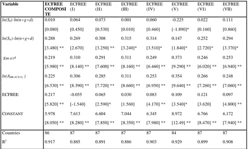
Tab. 4 The determinants of levels of income per working age person when indexes of economic freedom are included
Variable ECFREE COMPOSI TE ECFREE (I) ECFREE (II) ECFREE (III) ECFREE (IV) ECFREE (V) ECFREE (VI) ECFREE (VII) ln(Sk)-ln(n+g+d) 0.010 0.064 0.073 0.001 0.060 -0.225 0.022 0.111 [0.080] [0.450] [0.530] [0.010] [0.460] [-1.890]* [0.160] [0.860] ln(Sh)-ln(n+g+d) 0.288 0.269 0.308 0.315 0.314 0.147 0.252 0.294 [3.480] ** [2.670] [3.250] ** [3.240]* [3.510]* [1.840]* [2.720]* [3.370]* gBR-ICTt 0.219 0.310 0.291 0.311 0.249 0.373 0.246 0.253 [5.980] ** [8.140] ** [7.600] ** [8.160] ** [6.460] ** [9.290] ** [6.020] ** [6.940] ** ln(ABR-ICT(0) ) 0.225 0.306 0.285 0.311 0.253 0.354 0.266 0.248 [6.530] ** [8.390] ** [7.720] ** [8.660] ** [6.950] ** [9.640] ** [7.260] ** [7.060] ** ECFREE 0.217 -0.055 0.065 0.030 0.083 0.109 0.121 0.097 [5.820] ** [-1.540] [2.590]* [1.560] [4.170] ** [3.540]* [3.620] [4.800] ** CONSTANT 5.978 7.613 6.604 7.044 6.345 8.972 6.766 6.172 [8.050] ** [8.280] ** [7.850] ** [8.350] ** [7.980] ** [12.49] ** [8.470] ** [7.940] ** Countries 86 87 87 87 87 84 87 87 R2 0.917 0.885 0.891 0.886 0.903 0.929 0.899 0.908
The index of economic freedom published in the Economic Freedom of the World: 2000 Annual
Report is a weigthed average of the seven following composed indicators designed to identify the
consistency of institutional arrangements and policies with economic freedom in seven major areas: ECFREE(I) Size of Government: Consumption, Transfers, and Subsidies [11.0%], i) General Government Consumption Expenditures as a Percent of Total Consumption (50%), ii) Transfers and Subsidies as a Percent of GDP (50%). ECFREE(II) Structure of the Economy and Use of Markets (Production and allocation via governmental [14.2%] and political mandates rather than
private enterprises and markets) i) Government Enterprises and Investment as a Share of the
Economy (32.7%); ii) Price Controls: Extent to which Businesses Are Free to Set Their Own Prices (33.5%); iii) Top Marginal Tax Rate (and income threshold at which it applies) (25.0%); iv) The Use of Conscripts to Obtain Military Personnel (8.8%). ECFREE(III) Monetary Policy and Price Stability (Protection of money as a store of value and medium of exchange)[9.2%], i) Average Annual Growth Rate of the Money Supply during the Last Five Years (34.9%) minus the Growth Rate of Real GDP during the Last Ten Years; ii) Standard Deviation of the Annual Inflation Rate during the Last Five Years (32.6%); iii) Annual Inflation Rate during the Most Recent Year (32.5%). ECFREE(IV) Freedom to Use Alternative Currencies (Freedom of access to alternative
currencies) [14.6%] i) Freedom of Citizens to Own Foreign Currency Bank Accounts Domestically
and Abroad (50%); ii) Difference between the Official Exchange Rate and the Black Market Rate (50%). ECFREE(V): Legal Structure and Property Rights (Security of property rights and viability
of contracts) [16.6%] i) Legal Security of Private Ownership Rights (Risk of confiscation) (34.5%);
ii) Viability of Contracts (Risk of contract repudiation by the government) (33.9%); iii) Rule of Law: Legal Institutions Supportive of the Principles of Rule of Law (31.7%) and Access to a Nondiscriminatory Judiciary. ECFREE(VI) International Exchange: Freedom to Trade with Foreigners [17.1%] i) Taxes on International Trade, ia Revenue from Taxes on International Trade as a Percent of Exports plus Imports (23.3%), ib Mean Tariff Rate (24.6%), ic Standard Deviation
of Tariff Rates (23.6%), ii) Non-tariff Regulatory Trade Barriers, iib Percent of International Trade Covered by Non-tariff Trade Restraints (19.4%), iic Actual Size of Trade Sector Compared to the Expected Size (9.1%). ECFREE(VII) Freedom of Exchange in Capital and Financial Markets [17.2%], i) Ownership of Banks: Percent of Deposits Held in Privately Owned Banks (27.1%); ii) Extension of Credit: Percent of Credit Extended to Private Sector (21.2%); iii) Interest Rate Controls and Regulations that Lead to Negative Interest Rates (24.7%); iv) Restrictions on the Freedom of Citizens to Engage in Capital Transactions with Foreigners (27.1%).. Any of the
considered freedom indicators has a 0-10 value range. A higher value means a higher level in the item considered by the indicator .
T-stats are reported in square brackets.
** 95 percent significance with boostrap standard errors, * 90 percent significance with boostrap standard errors. We use the percentile and bias corrected approach with 2000 replications.
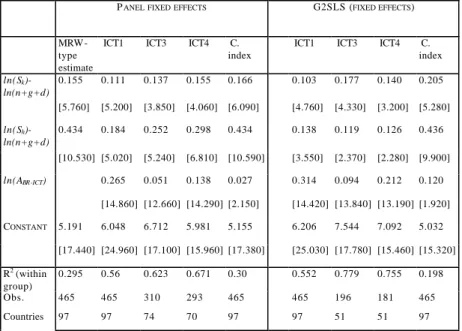
Tab. 5 The determinants of levels of income per worker estimated with panel data fixed effects and G2SLS fixed effects
PANEL FIXED EFFECTS G2SLS (FIXED EFFECTS)
MRW -type estimate
ICT1 ICT3 ICT4 C. index
ICT1 ICT3 ICT4 C. index ln(Sk)-ln(n+g+d) 0.155 0.111 0.137 0.155 0.166 0.103 0.177 0.140 0.205 [5.760] [5.200] [3.850] [4.060] [6.090] [4.760] [4.330] [3.200] [5.280] ln(Sh)-ln(n+g+d) 0.434 0.184 0.252 0.298 0.434 0.138 0.119 0.126 0.436 [10.530] [5.020] [5.240] [6.810] [10.590] [3.550] [2.370] [2.280] [9.900] ln(ABR-ICT) 0.265 0.051 0.138 0.027 0.314 0.094 0.212 0.120 [14.860] [12.660] [14.290] [2.150] [14.420] [13.840] [13.190] [1.920] CONSTANT 5.191 6.048 6.712 5.981 5.155 6.206 7.544 7.092 5.032 [17.440] [24.960] [17.100] [15.960] [17.380] [25.030] [17.780] [15.460] [15.320] R2 (within group) 0.295 0.56 0.623 0.671 0.30 0.552 0.779 0.755 0.198 Obs. 465 465 310 293 465 465 196 181 465 Countries 97 97 74 70 97 97 51 51 97
In the G2SLS panel estimate l n ( ABR-ICT )t is instrumented with ln(ABR-ICT )t -2, ln(ABR-ICT )t -3, and ln(ABR-ICT )t-4
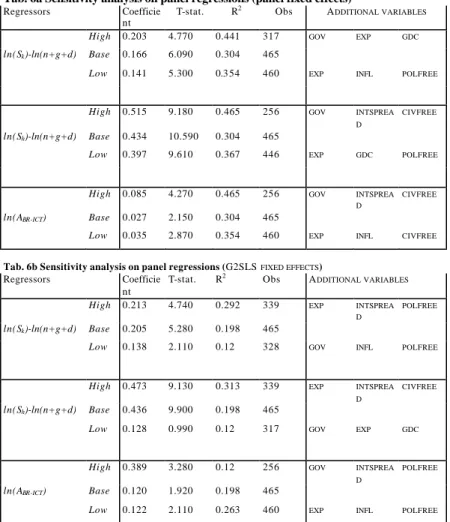
Tab. 6a Sensitivity analysis on panel regressions (panel fixed effects) Regressors Coefficie
nt
T-stat. R2 Obs A
DDITIONAL VARIABLES
High 0.203 4.770 0.441 317 GOV EXP GDC
ln(Sk)-ln(n+g+d) Base 0.166 6.090 0.304 465
Low 0.141 5.300 0.3 54 460 EXP INFL POLFREE
High 0.515 9.180 0.465 256 GOV INTSPREA
D
CIVFREE
ln(Sh)-ln(n+g+d) Base 0.434 10.590 0.304 465
Low 0.397 9.610 0.367 446 EXP GDC POLFREE
High 0.085 4.270 0.465 256 GOV INTSPREA
D
CIVFREE
ln(ABR-ICT) Base 0.027 2.150 0.304 465
Low 0.035 2.870 0.354 460 EXP INFL CIVFREE
Tab. 6b Sensitivity analysis on panel regressions (G2SLS FIXED EFFECTS)
Regressors Coefficie nt
T-stat. R2 Obs A
DDITIONAL VARIABLES
High 0.213 4.740 0.292 339 EXP INTSPREA
D
POLFREE
ln(Sk)-ln(n+g+d) Base 0.205 5.280 0.198 465
Low 0.138 2.110 0.12 328 GOV INFL POLFREE
High 0.473 9.130 0.313 339 EXP INTSPREA
D
CIVFREE
ln(Sh)-ln(n+g+d) Base 0.436 9.900 0.198 465
Low 0.128 0.990 0.12 317 GOV EXP GDC
High 0.389 3.280 0.12 256 GOV INTSPREA
D
POLFREE
ln(ABR-ICT) Base 0.120 1.920 0.198 465
Low 0.122 2.110 0.263 460 EXP INFL POLFREE
The sensitivity analysis is run by adding to the benchmark model all three by three combinations of the following variables: GOV: average government consumption to GDP, EXP : export to GDP, INFL:inflation, standard deviation of inflation, GDC: average growth rate of domestic credit;SD_GDC: standard deviation of domestic credit, ECONFREE: economic freedom, CIVFREE: civil freedom, LEGFREE: legal freedom, INTSPREAD: average difference between lending and borrowing rate in the domestic banking system.
In the table we select for each regressor of the base model only the benchmark estimate and the two replications in which the coefficient has the highest and the lowest significance.
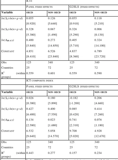
Tab. 7.a Subsample split results on panel regressions ICT1
PANEL FIXED EFFECTS G2SLS (FIXED EFFECTS)
Variable OECD NON OECD OECD NON OECD
ln(Sk)-ln(n+g+d) 0.055 0.126 0.055 0.118 [0.920] [5.6 60] [0.910] [5.210] ln(Sh)-ln(n+g+d) 0.328 0.067 0.326 0.006 [5.380] [1.490] [5.290] [0.130] ln(ABR-ICT) 0.400 0.273 0.405 0.324 [5.840] [14.850] [5.710] [14.100] CONSTANT 4.851 6.526 4.837 6.789 [8.410] [23.840] [8.360] [23.720] Obs 125 340 125 340 Countries 25 72 25 72 R2 (within groups) 0.559 0.601 0.559 0.590
ICT COMPOSITE INDEX
PANEL FIXED EFFECTS G2SLS (FIXED EFFECTS)
Variable OECD NON OECD OECD NON OECD
ln(Sk)-ln(n+g+d) 0.026 0.180 -0.182 0.206 [0.380] [5.890] [-1.200] [4.660] ln(Sh)-ln(n+g+d) 0.427 0.400 0.085 0.414 [6.400] [7.550] [0.420] [7.260] ln(ABR-ICT) 0.134 0.023 0.741 0.076 [2.580] [1.680] [2.310] [1.180] CONSTANT 6.532 5.058 9.708 4.928 [9.640] [14.570] [5.020] [12.670] Obs 125 340 125 340 Countries 25 72 25 72 R2 (within groups) 0.443 0.277 0.157 0.234
In the G2SLS panel estimate ln(ABRCT )t is instrumented with ln(ABRICT )t -2, ln(ABR-ICT )t -3, and ln(ABR-ICT )t-4
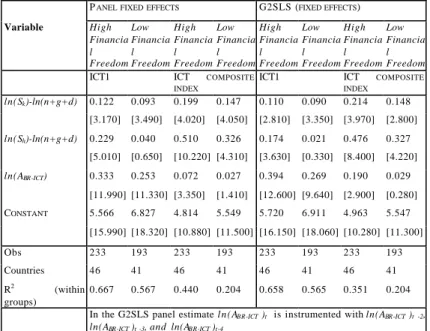
Tab. 7.b Financial market freedom, BR-ICT and growth on fixed effect and G2SLS panel regressions
PANEL FIXED EFFECTS G2SLS (FIXED EFFECTS)
Variable High Financia l Freedom Low Financia l Freedom High Financia l Freedom Low Financia l Freedom High Financia l Freedom Low Financia l Freedom High Financia l Freedom Low Financia l Freedom
ICT1 ICT COMPOSITE
INDEX
ICT1 ICT COMPOSITE
INDEX ln(Sk)-ln(n+g+d) 0.122 0.093 0.199 0.147 0.110 0.090 0.214 0.148 [3.170] [3.490] [4.020] [4.050] [2.810] [3.350] [3.970] [2.800] ln(Sh)-ln(n+g+d) 0.229 0.040 0.510 0.326 0.174 0.021 0.476 0.327 [5.010] [0.650] [10.220] [4.310] [3.630] [0.330] [8.400] [4.220] ln(ABR-ICT) 0.333 0.253 0.072 0.027 0.394 0.269 0.190 0.029 [11.990] [11.330] [3.350] [1.410] [12.600] [9.640] [2.900] [0.280] CONSTANT 5.566 6.827 4.814 5.549 5.720 6.911 4.963 5.547 [15.990] [18.320] [10.880] [11.500] [16.150] [18.060] [10.280] [11.300] Obs 233 193 233 193 233 193 233 193 Countries 46 41 46 41 46 41 46 41 R2 (within groups) 0.667 0.567 0.440 0.204 0.658 0.565 0.351 0.204
In the G2SLS panel estimate l n ( ABR-ICT )t is instrumented with ln(ABR-ICT )t -2, ln(ABR-ICT )t -3, and ln(ABR-ICT )t-4
Note: high financial freedom : countries ranked in the highest half according to the ECFREE (VII) indicator described in Table 4. Low financial freedom: countries ranked in the lowest half according to the ECFREE (VII) indicator described in Table 4.
Tab. 7.c Equity market development, BR-ICT and income per working-age person DEPENDENT VARIABLE: LOG GDP PER WORKING AGE PER SON 1997
PANEL FIXED EFFECTS
Variable High stock market development
Low stock market development
High stock market development
Low stock market development
ICT1 ICT COMPOSITE INDEX
ln(Sk)-ln(n+g+d) 0.071 0.060 0.209 0.087 [1.440] [2.120] [3.810] [1.930] ln(Sh)-ln(n+g+d) 0.249 -0.011 0.334 0.633 [4.950] [-0.170] [5.990] [8.410] ln(ABR-ICT) 0.336 0.325 0.219 0.031 [10.860] [14.030] [7.540] [1.510] CONSTANT 5.738 7.299 6.012 4.209 [13.470] [18.640] [12.000] [8.200] Obs 172 166 172 166 Countries 34 35 34 35 R2 (within groups) 0.654 0.758 0.544 0.396
Note: high equity market development: countries ranked in the highest half according to the stock market capitalisation to GDP indicator described in Table4. Low equity market development: countries ranked in the lowest half according to the stock market capitalisation to GDP indicator described in Table 4.
Tab. 8 Growth regressions with and without BR-ICT indicators DEPENDENT VARIABLE: LOG DIFFERENCE GDP PER WORKING AGE PER SON (1985-1997)
(1991-1997) (1983-1997) MRW -TYPE ESTIMATE EQUATION (1) WITH ICT1 EQUATION (1) WITH ICT3 EQUATION (1) WITH ICT4 EQUATION (1) WITH THE COMPOSIT E INDEX MRW EQUATION (1) WITH THE COMPOSIT E INDEX ln(Sk)-ln(n+g+d) 0.010 0.144 0.009 0.011 0.143 0.407 0.312 [4.818]** [3.080] ** [3.437] ** [4.903] ** [3.440] ** [5.140]** [4.370]** ln(Sh)-ln(n+g+d) 0.002 0.031 0.001 0.001 0.036 0.081 -0.0004 [2.814] ** [0.930] [1.146] [1.089] [1.280] [1.510] [-0.010] gBR-ICT 0.020 0.030 0.105 0.021 0.124 [0.790] [1.955]* [2.225]** [1.100] [5.500]** Ln(ABR-ICT(1985) ) 0.131 0.060 0.121 0.063 0.102 [3.040] ** [3.297] ** [4.199] ** [4.590] ** [4.500] Ln(Y/L)1985) -0.038 -0.041 -0.169 -0.240 -0.075 -0.095 -0.227 [-1.414] [-1.050] [-3.399] ** [-4.124] ** [-2.140] ** [-2.140]* [-4.630]** CONSTANT 0.170 -0.585 1.409 1.664 -0.1 71 -1.495 0.783 [0.857] [-1.410] [3.028] ** [3.457] ** [-0.420] [-4.010]** [1.330] R2 0.311 0.4208 0.520 0.557 0.4549 0.369 0.5346 Test: β=0 0.006 0.363 0.258 0.282 0.272 0.129 Implied λ 0.024 0.034 Countries 94 88 47 47 94 95 94
** 95 percent significance with boostrap standard errors, * 90 percent significance with boostrap standard errors. We use the percentile and bias corrected approach with 2000 replications.
Tab. 9 Sensitivity analysis on growth regressions (with composite BR-ICT indi cator) DEPENDENT VARIABLE: LOG DIFFERENCE GDP PER WORKING AGE PER SON (1985-1997)
Regressors Coeffici ent
T-stat R-sq Obs Additional variables
High 0.425 5.860 0.660 74 GOV INTSPREAD CIVFREE
ln(Sk)-ln(n+g+d) Base 0.312 4.370 0.535 94
Low 0.254 3.5 00 0.671 83 EXP SD_GDC ECONFREE
High 0.064 1.290 0.685 74 GOV EXP INTSPREAD
ln(Sh)-ln(n+g+d) Base 0.000 -0.010 0.535 94
Low -0.006 -0.110 0.662 84 EXP SD_INFL ECONFREE
High 0.094 4.060 0.553 91 EXP GDC CIVFREE
Ln(ABR-ICT(1985) ) Base 0.102 4.500 0.535 94
Low 0.070 3.260 0.685 74 GOV EXP INTSPREAD
High 0.115 5.060 0.553 91 EXP GDC CIVFREE
gBR-ICT Base 0.124 5.500 0.535 94
Low 0.093 4.220 0.660 74 GOV INTSPREAD POLFREE
High -0.206 -4.230 0.685 74 GOV EXP INTSPREAD
(Y/L)1985 Base -0.227 -4.630 0.535 94
Low -0.314 -6.260 0.670 83 EXP GDC ECONFREE The sensitivity analysis is run by adding to the benchmark model for growth estimated in Table 8 all three by three combinations of the following variables: GOV: average government consumption to GDP, EXP : export to GDP, INFL :inflation, standard deviation of inflation, GDC: average growth rate of domestic credit;SD_GDC: standard deviation of domestic credit, ECONFREE: economic freedom, CIVFREE: civil freedom, LEGFREE: legal freedom, INTSPREAD: average difference between lending and borrowing rate in the domestic banking system.
In the table we select for each regressor of the base model only the benchmark estimate and the two replications in which the coefficient has the highest and the lowest significance.