Estimation of the sharing rule between adults and children and related equivalence scales within a collective consumption framework

“

E

STIMATION OF THE

S

HARING

R

ULE BETWEEN

A

DULTS AND

C

HILDREN AND

R

ELATED

E

QUIVALENCE

S

CALES WITHIN

A

C

OLLECTIVE

C

ONSUMPTION

F

RAMEWORK

”

C

ARLOS

A

RIAS

, V

INCENZO

A

TELLA

, R

AFFAELLA

C

ASTAGNINI

,

AND

F

EDERICO

P

ERALI

CEIS Tor Vergata - Research Paper Series, Vol. 10, No. 28 August 2003

This paper can be downloaded without charge from the

Social Science Research Network Electronic Paper Collection:

http://ssrn.com/abstract=428540

CEIS Tor Vergata

R

ESEARCH

P

APER

S

ERIES

Estimation of the Sharing Rule between Adults and

Children and Related Equivalence Scales within

a Collective Consumption Framework

Carlos Arias, Vincenzo Atella, Raffaella Castagnini, Federico Perali

Abstract: In order to determine how much money is needed to make each household member as well off as they were before a change in living conditions, equivalence scales should be defined on the ba-sis of individual rather than household welfare. This requires the knowledge of individual utilities that are derivable from the identification of the rule governing the intra-household allocation of resources within a collective approach. We pursue this objective using information about male, female and chil-dren clothing expenditure present in the 1999 Italian Household budget survey within the estimation of a complete demand system. The sharing rule between adults and children is estimated using a structural rather than a reduced form approach. Maximum simulated likelihood is used to estimate a collective model of individual demand equations with zero expenditures for the exclusive good cloth-ing. The recovery of individual utilities for adults and children permits the estimation of the cost of children taking the intra-household distribution of resources into account. We show that the cost of Italian children is significantly affected by the parents’ aversion to intra-household inequality. Acknowledgments: The authors would like to thank Martina Menon, Eugenio Peluso, Marcella Veronesi and the participants to the Workshop on “Equivalence Scales, Household Behavior and Welfare” held in Florence 27-28 June 2002 for their helpful suggestions. All errors and omissions are the sole responsibility of the authors.

1 Introduction

The knowledge of utility functions of individual household members would permit refining the equivalence scale definition on the more correct basis of individual rather than house-hold welfare in order to determine how much money is needed to make each househouse-hold member, an adult or a child, as well off as they were before the change.

We pursue the objective of deriving individual utilities within the collective framework introduced by Chiappori (1988, 1992) using information about male, female and children clothing expenditure present in the 1999 Italian household budget survey within the estima-tion of a complete demand system. The sharing rule between adults and children is esti-mated using a structural rather than a reduced form approach. The system of structural equations presents a non negligible amount of zero expenditures for individual expenditures for clothing and education due to infrequent purchases. We account for non-consumption by implementing the method of maximum simulated likelihood.

As pointed out by Sen (1983), moving from inter-household to interpersonal compari-sons implies rejecting the assumption implicit in the traditional equivalence scales literature of either a “glued-together” family, or a “despotic family” taking the “dictatorial parents” indifference map as reference, or a family in which an egalitarian distribution equates the levels of well-being of the members. In Sen’s (1983:23) words, “A much more articulate family welfare function would then be needed to relate the collection of unequaled levels of well-being of family members to an aggregate measure for the family as a whole. This will, of course, involve a “mini social choice problem ... .” The approach of “equivalence scales” would have to be integrated more fully with intra-family allocation, on the one hand, and theories of aggregation of unequal well-beings, on the other.”

Gronau (1997:199-200) stresses this point asserting that “[...]. But it was left to re-searchers brought up in the tradition of home production to point out that the term "eco-nomic needs" does not exist in the eco"eco-nomics vocabulary, that the effect of children on con-sumption patterns depends on the intra-household redistribution of resources and consumption technology, and that in discussing “children-welfare indices” (which adult equivalence scales presume to be) one has to ask: whose welfare do we have in mind?”

This is still one of the main challenges for future research. According to Chiappori’s collective approach (1988, 1992), the recovery of individual utility functions requires the identification of the rules governing the intra-household distribution of resources. The knowledge of utility functions of individual household members would permit us to refine the equivalence scale definition on the more correct basis of individual rather than house-hold welfare in order to determine how much money is needed to make each househouse-hold member, be it an adult or a child, as well off as they were before the change. This is one of the main motivations underlying the present study.

This work is organized as follows. Section 2 introduces the demand specification within a collective consumption household model that adopts a technology that scales both prices (Barten 1964) and incomes (Gorman 1976) and accounts for corner solutions. The section also deals with the identification of the sharing rules and discusses the estimation possibilities between the rank and the property of income independence. Section 3 presents the 1999 ISTAT Italian budget data using nonparametric techniques for the estimation of the rank. Section 4 describes the econometric technique used to model zero expenditures.

The results are presented in section 5. The study ends with the conclusions and suggestions for future research.

2 The Collective Consumption Household Model

We define a family as composed by a married couple of adults a and, when present, chil-dren c. Adults are decision makers, paid or unpaid earners, and consumers. Chilchil-dren are consumers only. Both parents are altruistic towards their children in a paternalistic way. Children consumption enters parents' utility and children may be considered as public goods. Household members consume for their private use the vector of goods x∈ Nthat is composed by ordinary o, assignable si _{and exclusive e}i _{goods for i={a, c}.}1 _{The vector of} goods _x=

(

, ,_{o s e}i i

)

_{is additively separable inx=x}a_+xc_{. Individual consumption x}a _{and x}c

is not observed. Our objective is to use Chiappori's (1988, 1992) collective approach to es-timate the sharing rule governing the allocation of x to a and c.

A good is ordinary when a private good is consumed in unobserved proportions by all or some non identifiable household members. This is the common case given the informa-tion tradiinforma-tionally available in household expenditure surveys. It is conceivable that a survey could be specifically designed to record individual consumption, but it is costly and diffi-cult to trace individual consumption. This is why the collective research program has the ul-timate goal of recovering individual consumption from the observation of at least some in-dividual consumption commonly available in household expenditure or labour surveys. A good is assignable when a strictly private good is consumed in observed proportions by each member of the household. This may be the case when we can assign the consumption of clothing either to the adult or children component of the household but we cannot attrib-ute the consumption to either male and female adults. A less strict assumption is that one good can be observed as individually consumed with neither a public good nor an external component. A good is exclusive when a strictly private good is consumed by one identifi-able member of the household only. Notably, an assignidentifi-able good can be observationally equivalent to two, or as many members are in the households, exclusive goods. An example is clothing for adult males separate from adult females or separate from children and baby clothing, or alcohol and smoking consumption which, more properly, are adult bads.

As pointed out by Bourguignon, Browning, and Chiappori (1994), the distinction be-tween assignable and exclusive goods is particularly relevant when the available data re-ports detailed information about prices (or unit values are derivable). The price of exclusive goods are different for each household consumer, while prices are the same across house-hold members when goods are assignable.

In the collective consumption framework, the information set Ω known to the re-searcher is composed exclusively by information about consumption choices. In the collec-tive consumption set up, we assume that the vector of consumption goods _x∈ N _is

com-posed by at least two observable exclusive goods ea _{≥ 0 and e}c _{≥ 0, such as adult and}

1 In our notation superscripts denote endogenous variables, while subscripts index either exogenous variables or, in the case of functions, the derivatives of the endogenous variables.

children clothing, and one composite consumption good made up of the complement ele-ments of the set o∈ Nof market goods. Prices (or unit values) of the exclusive goods (pa ,

pc) are observable and exogenous. When the exclusive good is not consumed, then prices

are those prevailing in the market at a specific point of time.

The collective consumption setup assumes that the household is not engaged in house-hold production. Therefore, _T−li_=hi_{are hours of work supplied by each household}

mem-ber. Labour supply is assumed to be fixed as it is the case when the working members have a full time employment. Therefore, each member's earning wihi= yi is exogenous.

House-hold exogenous income y is then defined as the sum of adult and children expenditures plus non-labour income yo, y = ya + yc + yo. Then, the information set Ω available in a collective

consumption setting is:

(

)

{

, ; ; ; ;e e o h ya c i 0 p p p_a, _c;

}

∈Ω (1)

The collective household decision problem becomes:

( )

max_{U e o}i i, s.t. p e_i i+ ≤o φi

(

p p y y y_a, _c, _a, ,_{c o}

)

(2) , 0 , 0 > ≥ o ei

where

φ

i is the sharing rule governing the intra-household allocation of resources. The ex-istence of the sharing rule implies that we can recover individual consumptions xa _{and x}c_{. In}

contrast to the unitary model, marginal propensities to consume in the collective framework depend on individual incomes and are proportional to each other because they involve the sharing rule which is the same for all goods. The marginal effects depend on the amount of household resources allocated either to adults or children. Assignable goods are in general goods which must be observed at a high level of detail. In this situation, the occurrence of zero expenditures may be a problem making the collective consumption approach highly intractable. We devote next section to this problem.

2.1 Corner Solutions

A household or an individual facing a budget constraint may respond by either contracting the frequency of consumption, especially of luxury goods, or by tuning the personal trade-off between quantity/quality. A poor consumer may perceive more goods as “luxuries” rela-tive to rich consumers. Therefore, zero expenditures due to infrequent purchases during the recall period of the survey have a higher likelihood to be found in the consumption pattern of less well-off individuals. Accordingly, we assume that a zero realization is a genuine non consumption (Pudney 1990) modelled as the outcome of a Kuhn-Tucker corner solution.

If the utility function is well-behaved, the consumer must exhaust all her/his income so that at least one good, say the ordinary good, is consumed and the Lagrangean multiplier λ is greater than zero. Under this requirement, the necessary and sufficient first order condi-tions for a maximum are:

( )

, , i i o U e o =λ (3)

( )

,

( )

, 0, i i i i i o i e U e o −U e o p ≤ (4)

( )

,

( )

, 0, 0 i i i i i i i o i e U e o U e o p e e  ₋  _{= ≥}   , (5)

(

, , , ,

)

i i i a c a c o p e + =o φ p p y y y (6)

By complementary slackness, if _ei =0,_{, then:}

( )

( )

, , , i i i e i i i o U e o p U e o ≤ (7)

which says that the marginal rate of substitution between the exclusively consumed quanti-ties i (for i not equal 1) and the ordinary good 1 at the optimum is less than their price ratio. This condition can be rewritten as follows:

( )

( )

( )

, , ( ) , i i i i i i e e i i i i o U e o U e o v p U e o λ   = =       (8) where v_i(p_i) is the virtual price that would support a demand exactly equal to zero. If

equation (7) holds with strict inequality, then the virtual price described by equation (8) must be less than the market price. In this sense, the virtual price is a reservation price. Hence, a zero expenditure should correspond to a reservation price lower than the market value. From the Kuhn-Tucker set up, reservation prices, corresponding to the minimum price level at which consumers are willing to purchase the good, can be derived by invert-ing the system of the collective demand equations when the quantities consumed are zero.

The solution of the first order conditions yields demand functions of the form

(

)

*

( , ) ( , )

i _{p y X}i _{p y}

ξ = φ (9)

where _ξi( , )_{p y denotes a reduced form version of the demand and} *

(

)

( , )

i

X φ p y is the structural form explicitly including the sharing rule. The decision whether to consume or

not depends on the personal reservation price where the individual is indifferent between the two prospects. Pareto efficiency requires that both members are indifferent.

Definition 1. The double indifference property (consumption). On the consumption

fron-tier, member a is indifferent between consuming or not. Pareto efficiency then implies that member c is also on the consumption frontier (Blundell, Chiappori, Magnac, and Meghir 2001).

Here the consumption set is the set of price-income combinations such that a or c’s in-direct utility increases by consuming the good. At the frontier, the household is indifferent between consuming the good or not. This property guarantees that the sharing rule

(

, ,

)

i

a c

p p y

φ is a continuous function of both prices and income. In this setting, the deci-sions of one member depend on the market price of the other member’s consumption even in the case she/he is not consuming. Indifference is ensured by compensations, for the drop in welfare due to lack of consumption, through a positive transfer in consumption. The ex-istence of an interior solution to the above problem generates regular demand functions.

The present work specifies a collective demand system formally accounting for non-consumption. To be estimable, the sharing rule must be identified. We propose a structural approach.

2.2 The Household Decision Process: Identification of the Sharing Rule

This section introduces a novel approach which permits estimation of the sharing rule di-rectly from the structural specification. The technique is based on an analogy borrowed from the literature of modifying functions used to incorporating demographic or other ex-ogenous effects into demand systems (Pollak and Wales 1981, Lewbel 1985) and from studies estimating household technologies (Bollino, Perali and Rossi 2000). Similarly to sharing rules, demographic functions are not observable. In general, demographic functions interact with exogenous prices or income and can be identified provided that there is suffi-cient information in the data. Our analogy builds on the fact that, in order to achieve identi-fication from a structural speciidenti-fication, the unobservable sharing rule interacts with indi-vidual incomes a la Barten (Barten 1964, Perali 2003). The estimation problem is akin to the problem of estimating a regression containing unobservable independent variables (Goldberger 1972).

This approach, when practicable, is simpler than a reduced form approach (Chiappori, Fortin and Lacroix 2002). The latter approach can be very useful when the source of an identification problem of the parameters is lack of sufficient information in the data. We show that the information used in the econometric exercise is sufficient to identify the ex-ogenous parameters specified in the sharing function also using a structural approach.

The estimation of an individual demand function, as it is implied by a collective repre-sentation of the household decision process, requires the estimation of the sharing rule. The minimal informational requirement for the identification of the sharing rule is the ob-servability of at least one assignable good, or, equivalently, two exclusive goods. If one good is exclusive, and there are no externalities, for a given observed demand ( , )e p y satis-fying the Collective Slutsky property (Chiappori 1988, 1992 and Chiappori and Ekeland

2002a, 2002b)2 _{and such that the Jacobian ( , )}

p

D e p y is invertible, then the sharing rule

( , ) ( , ),

a p y p y

φ =φ φc( , ) 1_{p y} = −φ( , )_{p y} is identified up to an additive constant. The sharing

rule can be recovered by integrating back from the derivatives of the decision process. It is then possible to derive each member's demand for private goods, and the associated utility functions.

For illustrative purposes, we now follow the example developed by Chiappori, Fortin, and Lacroix (2002) adapting their notation related to the allocation of working time to our consumption set up. Instead of gender-specific supply of hours of work, we consider the consumption of clothing by the adults ea _{and the children e}c_{. The ordinary good completes}

the budget. The econometric identification of the sharing rule then consists in showing that the coefficients of a structural form correspond to the coefficients of an estimable, because unrestricted, reduced form. The demonstration that follows is functional to the estimation of the collective demand system in the empirical section.

The objective is to recover the partial effects

{

φ φ φ φ of the sharing rule: _pa, _pc, _yo, _s

}

a c o

p pa p pc y yo ss K

φ φ= +φ +φ +φ + (10) which is therefore identified up to an additive constant K. The constant K is the initial level from which the variations take place. It can be chosen arbitrarily without affecting the be-havioural information. Plausible candidates are the observed allocation y_a /y or the fair allocation y n/ where n is family size.

Let us first illustrate the source of the identification problem when undertaking the structural estimation of a collective model from the structural form. Consider the following specification which closely resembles the structure of Chiappori, Fortin, Lacroix (2002) along with the associated reduced form:

(

)

1 2 3 1 2 3 4 5 6 7 1 2 3 1 2 3 4 5 6 7 Re ln (.) ln ln ln ln ln ln ln ln ln (.) ln ln ln ln ln ln ln ln a a o o a c o a c o c c o o a c o a c o

Structural form duced form

e p d e f f p f p f y f p p f s f d f p e p y d e g g p g p g y g p p g s g d g p α α φ α β β φ β = + + = + + + + + + + = + − + = + + + + + + +

where ei _{is the consumption of clothing by individual i = a,c which indexes the adult and}

children component of the household respectively, pi is the price for the adult and child

good, po is the price of the ordinary good, y is non-wage income, s is the distribution factor

2 _{In presence of corner solutions, the Slutsky matrix should be more properly seen as an expected}

affecting only the decision rule but not preferences, d denotes other exogenous factors such as demographic characteristics. We choose a linear specification for the sharing rule φ : (.)

1 2 3 0 4

(.) lnp_a lnp_c lny ln .s

φ =γ +γ +γ +γ (11) Then, the demand for adult clothing becomes

1 2 1 2 3 0 4 3 1 1 2 3 0 4 3 1 2 1 2 2 2 3 2 3 4 2 4 ln ( ln ln ln ln ) ( ) ln ln ln ln ln ( ) ; ; ; . a m m f m m f e p p p y s d p p p y s d where α α γ γ γ γ α α ζ ζ ζ ζ α ζ α γ ζ α γ ζ α γ ζ α γ = + + + + + = + + + + + = = = = (12)

It is immediate to see that only the product of the parameters ζ_i =α γ_{2 i} for i=1,..,4 is identifiable unless α2 were known. The structural form, as it stands, does not allow the iden-tification of all the parameters of interest. The reduced form, on the other hand, is a feasible estimation strategy provided that the constraints linking the reduced form to the structure are known. What we propose is an indirect, but feasible, estimation of the structural form:

ˆ (.) (.) (.) ˆ (.) (.) (.) a a a c c a direct indirect y y y y y φ φ φ φ φ φ = = = − = − Note that (.) (.) (.) (.) (1 (.) c y a y ya ya yc ya yc ya φ = −φ = − φ = + − φ = + −φ ).

The indirect method is modelled as if it were a Barten equivalence scale (Barten 1964) and is anchored to ycwhich acts as if it were the additive constant. In the Barten model of

equivalence scales the demographic function modifying exogenous prices is unobservable as the sharing rule is.

Assumption 1 The income structure is specified as an income scaled term a la Barten

(1964)

( , , , , ).

i y m p p y z si a c o

φ =

By adopting this structure, the sharing rule φ can be interpreted as a shadow income (.)

post intra-household transfer where the scaling function m(·) describes the size and direc-tion of the symmetric transfer occurring between adults and children. The rule φa(.)is the

(.)

a a

y =φ as a separate equation and then insert it in the structure. For the indirect approach to be statistically viable, y_i must be exogenous as Barten prices in the Barten analogy. This structural assumption provides also crucial additional identifying information as the follow-ing proposition shows.

Proposition 1 For a given functional form of a collective demand system incorporating

As-sumption 1 and the associated unrestricted reduced form, both continuously differentiable, if the reduced form establishes a one-to-one correspondence with the structural form, then

the sharing rule _φa _{=φ can be identified up to an additive constant.}

Proof. By Assumption 1, we specify the structural and reduced form as follows:

(

)

1 3 2 1 2 3 4 5 6 7 2 1 2 3 0 4 Re ln ln ln ln ln ln ln ln ln ln ln ln ln ln ln a a o a o a c a o o a c

Structural form duced form

e p d y e f f p f p f y f y f s f d f p p p y s α α α α γ γ γ γ = + + + = + + + + + + + + + + + +

The unique correspondence between the structural and reduced form coefficients can be found by deriving the elements of the Jacobian matrix of the unrestricted reduced form and the corresponding elements of the Jacobian matrix of the structure which describes the theoretical restrictions relating the reduced form to the structure:

Structural form Reduced form

2 ln ln a a e y α ∂ = ∂ 2 1 ln ln a a e p α γ ∂ = ∂ 2 2 ln ln a c e p α γ ∂ = ∂ 2 3 ln ln a o e y α γ ∂ = ∂ 2 4 ln ln a e s α γ ∂ = ∂ 3 ln ln a a e f y ∂ = ∂ 1 ln ln a a e f p ∂ = ∂ 2 ln ln a c e f p ∂ = ∂ 4 ln ln a o e f y ∂ = ∂ 5 ln ln a e f s ∂ = ∂

By equating the corresponding elements of the Jacobian of the structural and reduced form and solving we obtain:

2 f3 α = 1 f1/ f3 γ = 2 f2/f3 γ = 3 f4/ f3 γ = 4 f5/ f3 γ =

where the unobservable γ parameters of the sharing rule in the structural form are a function of the observable f parameters of the reduced form.

Note that the correspondence has been established only for the unobserved γ parame-ters of the sharing rule, but it can readily be extended to all other parameparame-ters. This indirect structural approach has been empirically implemented within the estimated demand system expressed in shares as shown in the next section.

3 The Collective Quadratic Almost Ideal Demand System Modified a

la Barten-Gorman and Associated Equivalence Scales

In this section, we specify the identifiable model associated with the collective preferences described in the previous section. The knowledge of the sharing rule permits the derivation of individual indirect utility and cost functions that can be used to perform both interper-sonal and inter-household comparisons.

The demand system is an almost ideal demand model quadratic in the logarithm of total expenditure (Banks, Blundell, and Lewbel 1997). We made this choice with the purpose of cross-validating the non-parametric evidence presented in the next section which is in fa-vour of a rank two demand system with parametric tests. For the sake of generality, demo-graphic characteristics in our model interact multiplicatively both with prices and income in a theoretically plausible way (Lewbel 1985). The interaction with prices captures Barten-like substitution effects (Barten 1964); interactions with income captures Gorman-Barten-like fixed costs (Gorman 1976) representing the sum of the value of the good-specific committed quantities. The model is collective because it includes the sharing rule. Our specification exercise starts from the definition of individual indirect utilities according to the preference structure underlying the AIDS model.

Let the adult indirect extended PIGLOG utility function be:

1 1 ln( *) ln ( , ) ln ( , , ) ( , ) ( , ) a a a a Y A p d V Y p d p d B p d λ − − _{ − }    =__ _ + _     (13)

and the child indirect utility function: 1 1 ln( *) ln ( , ) ln ( , , ) ( , ) ( , ) c c c c Y A p d V Y p d p d B p d λ − − _{ − }    = _ _ + _{ }    (14) where: * * ln_Ya _=φa₋ln_PTa, ln_Yc _=φc₋ln_PTc ₍₁₅₎ and ln ln , ln ln a a c c a c w Y m w Y m φ = + φ = + (16) for lnm_c= −lnm_a. (17)

The logarithm of total expenditure is decomposed in lnY =walnY w+ clnY

forw_a =w_m+w_f where wm and wf are the shares of the male and female members of the

couple. The term λ( dp, ) is a differentiable, homogeneous function of degree zero in prices p. When independent of both prices and demographic characteristics, then the linear in income AIDS model is obtained.

Prices are scaled through Barten scaling to obtain shadow prices:

( )

*

lnpj=lnpj+lns dj . (18)

The vector of demographic characteristics can contain both individual and household specific attributes describing the household technology captured by the scaling demo-graphic function s d_j

( )

. When individual characteristics are included, then, individual shadow prices can be derived. To the individual shadow prices correspond the dual individ-ual shadow quantities q*_j =q s d_{j j}

( )

. The value of the scaling function s d_j

( )

=q q_j *_j

reveals the individual differences across household members in transforming a certain good into utility units. The transformation technology differs both across households and indi-viduals within the household.

Gorman’s committed income is a fixed cost translating income made up by the value of the good specific committed quantities tj (d):

(

)

( )

* 1 ln , ln N Ti j j j P p d t d p = =

∑

(19)

The fixed cost term lnPTi

(

p d,

)

is homogeneous of degree zero in p* _{. Similar to the}

Slutsky decomposition of substitution and income effects, the Barten-Gorman household technology rotates the budget constraint by modifying the effective prices with the substitu-tion effects (scaling) and translates the budget line through its fixed cost element (translat-ing).

In a collective setting, the definition of modified income _lnY* _=lnY−lnPT

where

a c

Y =Y +Y must accommodate the sharing rule as a function of exogenous prices p, non labor income y, exogenous household characteristics d, and extra-household factors z af-fecting the distribution rule without influencing preferences. We use the analogy with Bar-ten prices to define the sharing rule as a scaled income a

( )

. a

(

, , ,

)

a a c

Y m p p d z

φ = where

scaling function mi _{is specified in exponential form:}

(

, , ,

)

ln ln

(

, , ,

)

ln ln

(

a c

)

.

a a T

a c a a c a a c

p p d z Y m p p d z w Y p p d zθ θ ς

φ = + = + (20)

The income modifying function i

(

, , ,

)

a c

m p p d z has as arguments exogenous

informa-tion about the relative price of clothing for male and female, the difference in age between husband and wife, the difference in education level, and the rate of household separations in the region where households live acting as a distribution factor.

The scaling function of personal full income mi _{captures the size of the intra-household}

transfers. The sum shared between the adults and children is

(

1 a(.)

)

a

Y −m . The children get the rest. The amount offered

(

a(.) 1

)

a

Y m − corresponds to the amount received

(

1 a(.)

)

a

Y −m by the children. This specification of the distribution function explains how the virtual contract about the formation of individual expenditures realizes between adults and children. Notice that for a 0

a

Y Y m− > , then 0 a /

a

m Y Y

< ≤ . In the present context, identification of the sharing rule (up to a constant) comes from clothing consumed exclu-sively by the adults and the children.

The adult and child cost functions associated with the indirect utility functions are: ( ) ( , ) ln ( , , ) ln ( , ) ln ln 1 ( ) ( , ) a a a a T a a a u B p d C u p d A p d P m u λ p d = + + + − l l (21) and ( ) ( , ) ln ( , , ) ln ( , ) ln ln 1 ( ) ( , ) c c c c T c a c u B p d C u p d A p d P m u λ p d = + + − − l l (21)

In the tradition of the literature on demographic modifications of demand systems (Lewbel 1985), prices are scaled and incomes are translated. Here, incomes are both scaled, to estimate the sharing rule, and translated. Considering that our main objective is the esti-mation of the sharing rule from the observed consumption of exclusive goods, not the

re-covery of the effective individual consumption, in the present implementation, we drop the assumption of Barten prices. Therefore, p=p*_{. As a consequence, prices are the same for all}

household components. In accordance, we let the individual Translog price aggregator be equal across members as

lnA p da( , a) ln= A p dc( , c) 1 2ln ( ).= A p (23) Similarly, we assume that the Cobb-Douglas price term does not vary across members:

( , ) ( , ) 1 2 ( ),

a c

B p d =B p d = B p (24)

The term λ(p,d) is independent of demographic characteristics as well. The demo-graphic translating specification is instead maintained. The Gorman fixed cost term is re-stricted as follows:

lnPTa( ,p da) ln= PTc( ,p dc) 1 2 ln= P p dT( , ). (25) The household cost function is then derived as:

ln ( , , ) ln ( , , | ) ln ( , , |1 ) ( ) ( ) ( ) ( ) = ln ( ) ln ( , ) 1 ( ) ( ) 1 ( ) ( ) a m c m a a c c T a c C u p d C u p d C u p d u B p u B p A p P p d u p u p ϕ ϕ λ λ = + − = + + + − − l l l l (26) Roy's identity yields the estimated collective system of share equations:

(

)

(

)

(

)

(

)

* 1 2 * * 2 * * ( ) ln ln ln ( ) ln ln ( ) ( ) ln ln ( ) ln ln ( ) ( ) n i i i ij j j a a i i a a c c i i c c w a d p Y A p Y A p B p Y A p Y A p B p τ γ λ β λ β = = + + + + − + − + − + −

∑

(27) where _ln * a _ln T a Y =φ − P and _ln * c _ln T c

Y =φ − P . This is the estimated demand system. Note that this model is a first stage demand system with individual income effects. Another op-tion would have been to specify two separate collective individual demand systems having in common the sharing rule (Caiumi and Perali 2000).

Observed behaviour is then used to construct traditional equivalence scales and to evaluate how the cost of a child may depend on the intra-household distribution of re-sources. The traditional equivalence scale determines how much extra income is needed for a comparison household to reach the same level of utility as a reference household. When the profile of a reference and comparison household differ for a single characteristic, then the household scale reduces to a cost of characteristic. A household scale or cost of charac-teristic index is IB or Exact (ESE) if it only depends on prices and demographic

characteris-tics and is independent of the level of income chosen for comparisons (Lewbel 1989, 1991a, Blackorby and Donaldson 1991). As shown in Perali (2002), the equivalence scale for the Barten-Gorman AIDS model, with the IB property imposed, is the same whether it is linear or quadratic in the logarithm of income:

0 0 1 0 1 1 0 0 ( ( , , ), , ) ( , , ) ( , , ) ( ) ( , ) ( , ) ( ) ( , ) ( , ) IB T T T T C V Y p d p d ES u p d C u p d A p P p d P p d A p P p d P p d = = = = (28)

where the superscript 1 refers to the comparison household, while the superscript 0 indexes the reference household. When Barten substitution effects are absent, as it is in our case, the equivalence scale derived only from translating demographic effects is IB by construction. In a traditional equivalence scale, the sharing rule plays no role. The amount of resources transferred to the children is in our set up equal to the amount of resources that parents gave the children. It is an inter-household rather than an inter-personal comparison.

The cost of a child accounting for the intra-household distribution of resources, on the other hand, compares the members of two households having same income, facing same prices and with the same demographic composition in two different situations: a situation in which parents care more about their children, thus revealing a higher aversion to intra-household inequality, and a situation in which parents may, either out of necessity or delib-erate choice, care relatively less. We may also think at comparing the same household be-fore and after a permanent disability of one of the members.

We are then interested in determining how much is needed to a child living in a house-hold where parents have a low propensity to redistribute to attain the same level of utility of a child living in a household with a higher aversion to intra-household inequality, that is:

(

)

(

)

^ 1 0 0 ln , , ln , , c c c a c V Y p d = V Y Y m− p d     (29) where ln^ ln ln

(

₁

)

c a c t

Y = e + Y Y m− . If we insert expressions (13) and expression (14) and

solves for ln et, we obtain:

0 1

ln ln c ln c.

t

e = m − m (30) This equivalence scale, which does not depend on base income but it depends on the sharing rule, can be interpreted also as an equivalent transfer. The amount that establishes the equality in welfare levels across two similar children in two households differing for their redistributive behaviour corresponds to the difference in the adults to children trans-fers of resources.

Data Description and Characteristics

The data used for this paper are drawn from the ISTAT 1999 cross-sectional household survey. We selected households composed by married couples with dependent children aged 0-17. Both spouses work full-time. The sample includes 836 households. Several goods in the ISTAT 1999 survey are consumed exclusively by adults or children. The ex-penditure for clothing is assignable to the husband, the wife and the children. The availabil-ity of assignable goods is crucial to identify the rule governing the distribution of resources within the household. We consider only expenditures on non durable goods. The expendi-ture categories are food, household operation, education and leisure, clothing for men, clothing for women, clothing for children, and other consumption. Household-specific prices have been assigned to each household following the procedure to estimate unit val-ues also in the absence of quantity information described in Atella, Menon, and Perali (2003). A detailed description of the aggregated categories, separated in terms of the possi-ble classification into private, public, assignapossi-ble, exclusive and adult or children good, is provided in Table 1.

Table 2 reports the descriptive statistics of the sample. The aggregate goods included in the analysis are Food, Household Operations, Education and Recreation, Clothing for men and women, Clothing for Children and Other Consumption. The set of demographic vari-ables includes the macro-regions (North-West, North-East, Center, South), the number of children in different age categories (0-5, 6-14, 15-17), a dummy variable taking the value of 1 if the household is female-headed, a dummy for the winter term to capture seasonality in clothing consumption, and a dummy variable that is equal to one when the education of the household head is at least at college level. The exogenous household characteristics in-cluded in the sharing rule are the ratio between the wife’s age and the total age of the two spouses, the ratio between the years of schooling of the wife and the total years of school-ing of the spouses. We also included an extra-household environmental parameter given by the number of legal separations per thousand married couples for each of the twenty Italian regions.

The expenditure shares on education, clothing for men, women, and children report a non negligible amount of censoring. This is partly explained by the short length of the re-call period of the survey design and partly as the result of genuine non-consumption (Pud-ney 1990). The recall period for clothing is one month. As Grosh and Glewwe (2000) pointed out, the choice among recall periods is one of the most important and difficult de-sign issues for a consumption model. A longer recall period may suffer from under-reporting.

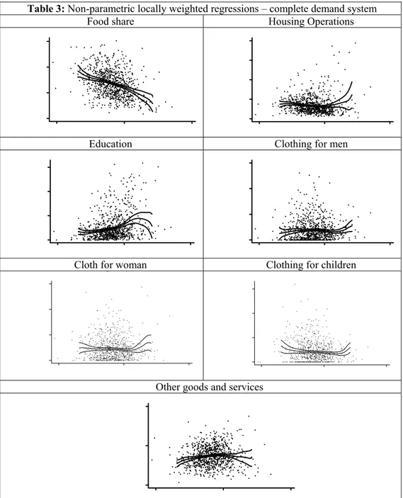
We investigate the shape of the Engel curves and the rank of the demand system as a data description tool and with the objective to learn some priors about a specification of the demand system capable of interpreting the data correctly. The non-parametric smoother that we use is a local linear fit (Fan 1992, Fan and Gijbels 1996) which proves to be a superior linear smoothers in regions where data are scarce. Other smoothers such as the Nadaraya-Watson generate a large bias when estimating a curve at a boundary region.

The findings of the nonparametric analysis gathered in Table 3 can be summarized as follows. As it is reasonable to expect, the Engel curve for Food is linear along the whole range of the income/expenditure distribution. In the case of Household operation, the

re-gression curve shows some degree of non-linearity at the boundary regions although the overall shape of the curve is almost flat.

This share is in average 13.7 percent of the budget of Italian households. The relative budget weight of goods showing non-linear Engel curves is important because the outcome of the rank test is sensitive to the size of the share. This implies that a non-linear small share within the demand system may not be sufficient to justify a rank three demand system which hosts a quadratic income term.

Table 1

Classification of Goods and Aggregation

Group Public Private

Exclusive Ordinary

Adults Children

Food at home Tobacco Non-alcoholic

beverages Alcoholic beverages

Food

Food away from home Electricity, gas, fuel oil

and coal

Semi-durable fur-nishing Domestic services Water and sanitary _services Household cleaners and

supplies Telephone

Housing Operations

Other household opera-tions

Magazines and

newspapers Tuition for school Movie theatre, and

spectator sports School books Toys and sport

equipment

Other exp. for education Holidays and trips

Education and Recreation

Other recreation

Men clothing Children clothing Men shoes Children shoes Men other apparels Women clothing Women shoes Clothing Women other apparels Communication Medical care Personal care Other Goods Transportation

Table 2

Descriptive Statistics – No. of obs. 836

Trunc. % Mean Std. Dev. Min Max

Shares

Food 0 0.270 0.104 0.035 0.605

Household operations 0 0.137 0.090 0.011 0.777

Education and Recreation 2.87 0.103 0.110 0.000 0.636 Clothing for men 16.03 0.037 0.041 0.000 0.262

Clothing for women 11.01 0.045 0.044 0.000 0.288 Clothing for children 22.01 0.041 0.043 0.000 0.320 Other consumption 0 0.367 0.130 0.032 0.876 Expenditures and Prices

Total expenditure 2322.901 647.103 318.659 5254.162 Husband total expenditure 673.888 235.888 49.148 1749.877 Wife total expenditure 690.034 241.632 55.834 1779.393 Children total expenditure 958.979 376.110 109.159 2314.640

Food 4.522 1.661 1.312 10.283

Household operations 19.914 12.698 4.151 69.083 Education and Recreation 1.136 1.071 0.064 4.051

Clothing for men 1.485 1.239 0.175 5.263

Clothing for women 1.589 1.339 0.181 5.635 Clothing for children 0.595 0.081 0.439 0.860 Other consumption 4.398 3.242 0.560 17.606 Demographic variables North-East 0.286 0.452 0 1 North-West 0.292 0.455 0 1 Center 0.184 0.388 0 1 South 0.175 0.380 0 1 No. of children 0-5 0.596 0.630 0 3 No. of children 6-14 0.836 0.746 0 3 No. of children 15-17 0.139 0.366 0 2 Separation ratio 1.093 0.287 0.422 1.427

Seasonal dummy - Fall=1 0.264 0.441 0 1

High Education 0.519 0.500 0 1

Wife - household head 0.036 0.186 0 1

Age ratio 0.483 0.020 0.387 0.558

Table 3: Non-parametric locally weighted regressions – complete demand system

Food share Housing Operations

Education Clothing for men

Cloth for woman g p Clothing for children

Other goods and services

The shares of Clothing for males, females and children do not vary substantially with the level of total expenditure, although the width of the bootstrapped confidence bands for Clothing for women shows greater variability. The Education and Recreation share is linear and upward sloping. As expected, the locally weighted nonparametric regression of the composite share of other consumption goods shows a non-linear shape.

The investigation of the most appropriate functional form for the demand system was further explored applying the nonparametric test of the rank of a demand system introduced by Lewbel (1991b, 1997). The results of the rank test applied to our sample presented in Table 4 support a rank of two. We proceed sequentially by examining whether the rank of the demand system is r = 1, that is evaluating the null hypothesis that only pivot d1 is

sig-nificantly different from zero, and consequently, all remaining six pivots are zero. We re-ject the null because the probability to have χ2 _{with six degree of freedom less than 10.93 is} less than 10%.Therefore, the rank is greater than one. From the inspection of column d = 2 and r = 3, we see that the second pivot is significantly different from zero. The null hy-pothesis that all remaining five pivots are zero is accepted. The statistics χ2

(0.01, 5) is less then the critical values 15.09. The probability that all but two pivots are zero is 99 percent. The combination of the results of the nonparametric locally weighted regression and the rank test indicate that a linear specification of the demand system is probably the most ap-propriate for the overall demand system even if some degree of non-linearity is present in some goods of the Italian basket particularly in the tails of the distribution.

In order to test whether there is consistency between the non-parametric and parametric evidence, we decided to estimate a demand system quadratic in the logarithm of total ex-penditure. On the basis of the non-parametric evidence, we expect that most of the parame-ters associated with the quadratic income term are not statistically significantly different from zero.

It is interesting to note that there is a direct connection between the rank of a demand system and the property of independence of the base level of utility or income chosen for interpersonal comparisons (Lewbel 1989 and 1991, Blackorby and Donaldson 1991, Pen-dakur 1999). If two adjacent Engel curves referring to household types differing for one characteristic are shape invariant and linear, then the two Engel curves of interest are also parallel. It follows that the vertical distance between the curves does not vary across income levels. Equivalence scales are therefore exact in the sense that they are independent of the income level chosen as a reference for comparisons.

Econometric Method

In this section, we review two feasible methods of estimation for systems of equations with multiple censored variables. The generalized Heckman procedure is an extension to a system of equations of the two-step Heckman estimator (Heckman 1974 and 1979), while the maximum simulated likelihood method (Hajivassiliou, McFadden and Ruud 1996) uses multiple integrals that are computed with a simulated algorithm to reproduce the statistical process that generated the zero realizations. Both methods provide unbiased estimates of the structural parameters. However, in the simulated maximum likelihood approach the variance-covariance matrix of the random disturbances of the latent variables in the cen-sored model is a full matrix. In other words, it is possible to explicitly model the correlation

among the random disturbances of the latent variables of a censored system. On the other hand, in the case of the generalized Heckman estimator only the diagonal terms (the vari-ances of the latent variables) can be estimated. In this paper, we estimate reasonable start-ing values for the maximum simulated likelihood estimation usstart-ing the estimates of the gen-eralized Heckman procedure which is computationally less demanding.

Table 4

Nonparametric Rank Test

Pivots χ2 _{statistics and p-values}

d=1 d=2 d=3 d=4 r=1 r=2 r=3 r=4 0.657 -0.105 -0.010 -0.002 10.93 0.185 0.002 0.000

0.141 0.999 1 1

Note: The four largest pivots d are reported. The remaining three pivots are zero to three or more decimal

places. r denotes the rank being tested. The test is that all pivots, except the rth _{largest pivot, are zero.} Each test is consistent only against alternatives that the rank is greater than r. The degrees of freedom of the statistic are 7-r. The p-values of the χ2 _{distribution are in italics.}

We describe the two proposed estimation methods using a general representation of a system of equations with censored endogenous variables. Each equation in the system can be written as: ( , ) if ( , ) 0 0 if ( , ) 0 i i i i i i i i i i i i i i y f x u f x u y f x u β β β = + + > = + < (31)

where, yi is the endogenous variable corresponding to the i-th equation in the system, xi is a

vector of explanatory variables, βi is a vector of parameters and ui is a random variable.

Precisely, ui is the i-th component of a multivariate normal random vector u of mean zero

and variance Σ. Therefore,

2 ~ (0, )

i i

u N σ

where, σi2 is the i-th diagonal term of the matrix Σ.

Generalized Heckman Estimator

This procedure amounts to transform the system of censored equations in (31) into a system of uncensored equations by using the appropriate correction. Let us consider the un-conditional mean (un-conditional only on explanatory variables):

[ | ] [ | 0] ( , ) ( , ) ( , ) ( , ) i i i i it i i i i i i i i i i i i i i i f x E y x E y y f x f x f x β σ β β β σ φ σ σ   = > Φ =       = Φ +       (32)

where, φ and Φ are respectively the probability density function and the cumulative density function of a standard normal distribution. Using the expression for the unconditional ex-pected value of each endogenous variable we consider the following system of uncensored equations: ( , ) ( , ) ( , ) i i i i i i i i i i i i i i f x f x y f x β β σ φ β ξ σ σ     = Φ +  +     (33)

where ξ =_it y_it−E y x

[

_i | _it

]

. The system in (32) can be estimated by limited maximum like-lihood assuming that:

~MVN(0, )

ξ Ω

where, ξ is a random vector which i-th element is ξi. An important detail is that this is a

straightforward maximum likelihood estimation since the system in (32) does not contain any censored equation. From equation (32), it is clear that only the variances of the random disturbances of the latent variables in the censored system described in expression (30) get estimated. In fact, the off-diagonal terms of the matrix Σ do not appear in expression (32). In this sense, it is important to note that the random disturbances of the observed variables in the uncensored system in (32) are different from the random disturbances of the latent variables in expression (30). We use this approach to generate reasonable starting values for the method of simulated maximum likelihood.

Simulated Maximum Likelihood

In this section, we discuss the likelihood function of a system of censored equations. As we will see below, the characteristics of the associated likelihood function has precluded the use of this estimation procedure in empirical papers. The likelihood function of the sys-tem in (30) when all endogenous variables are above their censoring levels is given by:

1 ( , ... ,1 m)

L =df u u

where the ui's are the random disturbances of the system in (30) and df is the probability

density function of a multivariate normal random vector with mean zero and variance Σ. The likelihood function for an observation in which the n first endogenous variables out of

1 2 1 1 1 1 1 1 1 1 c cn m n c cn n+ m n n+ m n

L ... df(u ,...,u )du ...du

df (u ,...,u ) ... cf(u ,...,u | u ,...,u )du ...du

−∞ −∞ −∞ −∞ = = =

∫ ∫

∫ ∫

(33)

where, dfi is the marginal probability density function of the uncensored portion and cf is

the probability density function of the censored variables conditional on the uncensored ones. Expression (33) represents a portion of the likelihood function with an n-dimensional definite integral. Under the assumption of multivariate normality of the disturbances of the system this integral does not have a close form solution. Therefore, estimating the system of equations by maximum likelihood requires an efficient method for evaluating the high dimensional definite integrals. Maximum Simulated Likelihood (SML) consists on simulat-ing rather than calculatsimulat-ing these integrals ussimulat-ing probability simulation methods.

Probability simulation methods are based on the fact that the integral of interest repre-sents the probability of an event in a population. Lerman and Manski (1981) propose gener-ating a pseudo-random sample of observations from the relevant population and using the relative frequency of the event in the sample to approximate the integral of interest. This simulation method is called a “crude frequency simulator” and it was improved in several subsequent papers. Stern (1992) explains the importance of smoothness in a probability simulator and proposes an smooth alternative to the “crude frequency simulator.” Geweke (1989) and Borsh-Saupan and Hajivassiliou (1993) proposed the GHK simulator. Hajivas-siliou, McFadden and Ruud (1996) find that the GHK probability simulator outperforms all other methods by keeping a good balance between accuracy and computational costs.3

Results

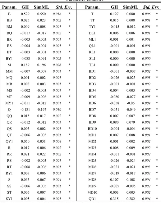
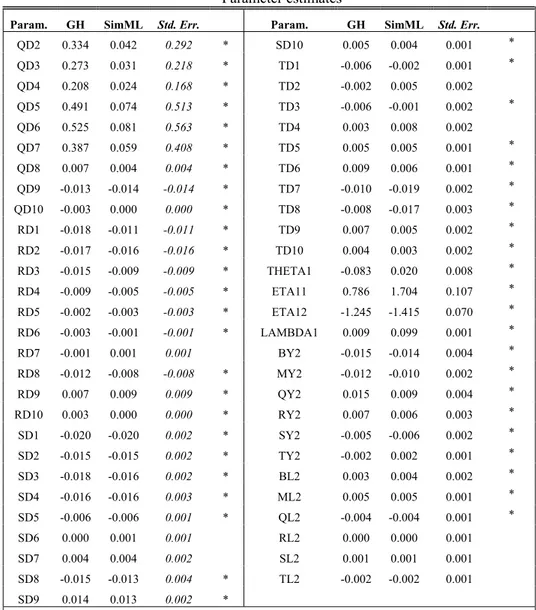
This section describes the estimates of the Quadratic Almost Ideal Collective Demand System (QAICDS) obtained using the method of simulated maximum likelihood to account for zero expenditures and the derived equivalence scales conditional upon the intra-household distribution of resources. Identification of the sharing rule requires that individ-ual and household total expenditure are exogenous. Expenditures can be endogenous be-cause of measurement errors arising from infrequency of purchase and, especially in the context of a collective model, simultaneity. Table A.1 in the appendix reports the results of the Hausman-Wu tests conducted following the general methodology illustrated in Mroz (1987).

Total expenditure is endogenous in the Food, Housing and Education shares and ex-ogenous for the Other goods share. Total expenditure is exex-ogenous in all types of clothing. However, total expenditure for men is endogenous in the equation Clothing for men and is exogenous in the equation clothing for women. Symmetrically and in line with our expecta-tions, total expenditure for women is endogenous in the equation clothing for women and exogenous in the equation clothing for men. Individual expenditures are exogenous in the equation clothing for children. In general, it is important to point out that the

tion of expenditure is a delicate exercise. Instrumentation should preserve the main features of the original distribution. If not, we may experience a change in the true rank of the de-mand system (Blundell and Duncan 1998, Blundell, Duncan and Pendakur 1998, Gozalo 1997, Lyssiotou, Pashardes and Stengos 1999) and a loss of important features when meas-uring child costs such as the monotonicity of total expenditure with respect to children.

The Quadratic Almost Ideal Collective Demand system has been estimated using the Generalized Heckman procedure to obtain reasonable starting value for the Simulated Maximum Likelihood procedure. The system has been estimated with the properties of symmetry and homogeneity as maintained hypothesis. The Slutsky matrix has two individ-ual income terms which sum to the household level income effect because of the symmetry of the individual transfers as shown in equation (17).

Table A.2 reports the estimated parameters of the collective demand system described in equations (27). We report the starting values generated using the Generalized Heckman procedure and the parameters obtained using simulated maximum likelihood along with the associated standard errors. The parameters are in general significantly different from zero including the parameters associated with the factors of the sharing rule (THETA1, ETA11, ETA12, LAMBDA1). Interestingly, the parameters associated with the quadratic income term (BL1, ML1, QL1, RL1, SL1, TL1 and BL2, ML2, QL2, RL2, SL2, TL2) are in gen-eral not significantly different from zero pointing to the fact that the Engel space underlying the estimated demand system can be rank two. The value of the Likelihood Ratio Test of 19.73 comparing the Individual Model Quadratic in Income (CQAIDS) with respect to the Individual Demand System Linear in Income (CAIDS) shows that the quadratic specifica-tion is not statistically superior to the linear specificaspecifica-tion at the .05 level of significance (χ2

(12)=21.03 where 12 are the degrees of freedom). These results are in line with the non-parametric test of the rank reported in the previous section. This initial evidence about the shape of individual Engel curves should be the subject of further empirical investigation.

Table 5 reports the compensated price and income elasticities computed at the data mean using numerical procedures. Note that all elasticities are unconditional in the sense that incorporate also the impact on the probability to consume. The estimated demand sys-tem is regular and economically meaningful. The compensated own price elasticities are of the correct sign. The good most responsive to income is education and leisure. Expenditures on clothing for children are more necessary than expenditures on clothing for adults.

Demographic effects reported in Table 6 are of the translated type. The number of chil-dren has a negative impact on food. This sign is explained by the instrumentation of total expenditure. Nonparametric analysis of Engel curves varying for an increasing number of children conducted using non instrumented total expenditure shows Engel curves moving to the right as family size increases. The other demographic effects are in general consistent with expectations.

Table 7 shows the predicted values of the sharing rule evaluated at the household spe-cific constant Ya ma/Y as the number of children in the household increases. When only one

child is present in the household, the adults hold for their own consumption 46.5 percent of the household resources. In households with two children, each child receives 34 percent of the household resources which is less than the 53.5 percent of household resources received by a single child. With three children, each child receives 26 percent of household re-sources which is slightly higher than the fair allocation of 20 percent in a household of five members.

Table 5

Unconditional Compensated Price and Income Elasticities

Unconditional Compensated Price Elasticity Food Housing Education and

Leisure Clothing for man Clothing for woman Clothing for Children Other goods Income Elasticity Food -0.561 0.183 0.010 0.023 0.031 0.055 0.360 0.880 Housing 0.329 -0.920 0.112 0.056 0.026 -0.020 0.417 0.992 Education and Leisure -0.030 0.106 -0.711 -0.066 0.066 -0.044 0.519 1.238 Clothing for man 0.099 0.161 -0.135 -0.498 0.005 -0.166 0.399 1.137 Clothing for woman 0.170 0.082 0.175 0.007 -1.081 0.159 0.500 1.015 Clothing for children 0.373 0.024 -0.037 -0.110 0.155 -0.652 0.498 0.755 Other goods 0.212 0.135 0.159 0.042 0.058 0.048 -0.671 1.034 Table 6 Demographic Elasticities Food Housing Education and Leisure Clothing for man Clothing for woman Clothing for

chil-dren Other goods

North-West -0.041 0.054 0.415 -0.394 -0.389 -0.104 0.002 North-East -0.108 0.007 0.451 -0.379 -0.294 -0.060 0.032 Center -0.012 0.063 0.357 -0.338 -0.352 -0.106 -0.015 South 0.009 -0.007 0.280 -0.201 -0.323 0.049 -0.026 No. of children < 6 -0.342 -0.202 0.711 -0.017 -0.122 0.016 0.110 No. of children 6-14 -0.259 -0.179 0.759 -0.033 -0.008 0.073 0.013 No. of children 15-17 -0.222 -0.148 0.552 -0.001 0.070 -0.231 0.066 Wife - household head 0.040 0.119 0.037 -0.282 -0.308 -0.113 0.012 Seasonal Dummy - Fall=1 0.040 -0.036 -0.112 0.169 0.279 0.106 -0.054 High Education -0.018 0.023 -0.028 0.077 0.109 0.071 -0.021

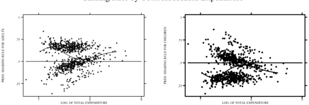
The panels in Fig. 1 show how the estimated sharing rule varies in relation to total household expenditure. The first graph, representing the level of the sharing rule

(

/

)

a a

Y Y m , is a mirror image of the second graph representing the amount of transfers

re-ceived by the children from the adults

(

/

)

(

1 a

)

a

Y Y −m . The graph shows that households with lower levels of total household expenditures have a lower propensity to transfer re-sources to children.

Table 7

Predicted Sharing Rule of Adults by Number of Children

Children Mean Std. Dev. Min. Max.

1 0.465 0.262 0.388 0.583 2 0.322 0.419 0.169 0.429 3 0.219 0.549 0.094 0.353

Fig. 1

Sharing Rule by Total Household Expenditure

P R ED. S HAR ING R U LE F O R ADULTS

LOG. OF TOTAL EXPENDITURE

7 8 9 .25 .5 .75 1 P R ED. S HAR ING R U LE F O R C H ILDR EN

LOG. OF TOTAL EXPENDITURE

7 8 9

.25 .5 .75 1

Fig. 2 describes how the propensity to transfer resources to children in the Italian households is affected by changes in the separation rates in the Italian regions. The graph shows that at low and high levels of separation rate, the adults hold more resources for themselves. This mixed effect suggests that the different separation rates observed in the Italian regions is a factor that may affect bargaining decisions between husbands and wives, but does not significantly affect the degree of aversion to intra-household inequality and the polarization between adults and children.

In order to determine how much money is needed to make each household member as well off as they were before a change in living conditions, equivalence scales should be de-fined on the basis of individual rather than household welfare. The collective nature of the estimated demand system allowed us to derive both a household and an individual cost and indirect utility function as described in the methodology section. Table 8 presents tradi-tional equivalence scales representing the index of the cost associated with the characteris-tic “presence of a child of a certain age.” Younger children are about 23 percent of the cost of a childless couple and about 46 percent of an equivalent adult. Older children cost about 60 percent more and are about 80 percent of the cost of an equivalent adult. The cost of a

child proposed in Table 8 is independent of the base level of income chosen for comparison because demographic information has been introduced in the demand system as a translat-ing effect. Table 9 describes a measure of the variation in relative utility levels associated with shifts in the distribution of power. In households where mothers are more educated the transfer to children are higher. Children are relatively less well-off in households with rela-tively older household heads with respect to the other partner’s age. The separation rate and the relative price of cloths seem less important in affecting individual levels of well-being. This information may be used also to infer the amount of effective basic resources actually received by children in relation to the redistributive behaviour and the degree of caring of the Italian households.

Fig. 2

Sharing Rule and Rate of Separation

PRED.

SHARING RULE FOR ADULTS

RATE OF SEPARATION .5 1 1.5 0 .2 .4 .6 .8 Table 8

The Traditional Cost of a Child Child age Cost of a child

0-5 1.24 6-14 1.22 15-17 1.39

The recovery of individual utilities for adults and children permits the estimation of cost of children taking the intra-household distribution of resources into account. In fact, while the traditional cost of a child does not depend on income, a cost of a child accounting for the distributive behaviour for the adults does depend on the sharing rule. We use then the definition provided in equation (29) to determine the equivalent transfer necessary to guarantee the same welfare level to two children living in the same or similar households in two different redistributive situations. Let us take the minimum and maximum value of the

predicted sharing rule of households with one child presented in Table 7 as an example of two different redistributive situations, everything else hold equal. The compensation to be given to the child living in the household where less is distributed is

0 1

lnet =lnmc−lnmc=0.58 0.38 0.2− = of the reference level of income. This example shows that parent’s aversion to inequality may significantly affect the actual cost of a child and level of children’s utility.

Table 9

. The Indirect Utility Ratio between Adults and Children

(½ Va_)/Vc

+10% 1.034

Separation ratio 1.036

Age ratio 1.083

Education ratio 0.903

Clothing price ratio 1.035

Conclusions

This paper uses an indirect structural approach to identify the sharing rule between adults and children of the ISTAT 1999 sample of Italian households. The identification of the sharing rule within a Collective Demand System which accounts for economic non-consumption permitted recovering individual utilities. Knowledge of the sharing rule pro-vides information about the intra-household distribution of power. When making welfare comparisons it is desirable to implement them across households or individuals with a simi-lar propensity to redistribute resources among the household members. We therefore report equivalence scales distinguishing among Italian household where adults are more or less prone to transfer resources to their children. We show that the cost of Italian children is sig-nificantly affected by the parents’ aversion to intra-household inequality.

The structural approach to the estimation of the sharing rule pursued in this study can be extended to the joint estimation of both the rule governing the horizontal transfers be-tween husband and wife and the vertical transfers bebe-tween adults and children. It should be stressed that the estimated collective system of individual demands is just one member of a family of collective demand systems yet to be characterized.