2016
Publication Year
2020-05-19T08:33:49Z
Acceptance in OA@INAF
Analytical model of Europa's O2 exosphere
Title
MILILLO, Anna; PLAINAKI, CHRISTINA; DE ANGELIS, Elisabetta; MANGANO, VALERIA; MASSETTI, Stefano; et al.
Authors
10.1016/j.pss.2015.10.011
DOI
http://hdl.handle.net/20.500.12386/24947
Handle
PLANETARY AND SPACE SCIENCE
Journal
130
Analytical model of Europa’s O
2
exosphere
Anna Milillo ([email protected]), Christina Plainaki, Elisabetta De Angelis, Valeria Mangano, Stefano Massetti, Alessandro Mura, Stefano Orsini, Rosanna Rispoli
INAF/Istituto di Astrofisica e Planetologia Spaziali, via del Fosso del Cavaliere, 00133 Rome, Italy
Abstract
The origin of the exosphere of Europa is its water ice surface. The existing exosphere models, assuming either a collisionless environment (simple Monte Carlo techniques) or a kinetic approach (Direct Monte Carlo Method) both predict that the major constituent of the exosphere is molecular oxygen. Specifically, O2 is generated at the
surface through radiolysis and chemical interactions of the water dissociation products. The non-escaping O2 molecules circulate around the moon impacting the
surface several times, due to their long lifetime and due to their non- sticking, suffering thermalization to the surface temperature after each impact. In fact, the HST observations of the O emission lines proved the presence of an asymmetric atomic Oxygen distribution, related to a thin asymmetric molecular Oxygen atmosphere. The existing Monte Carlo models are not easily applicable as input of simulations devoted to the study of the plasma interactions with the moon. On the other hand, the simple exponential density profiles cannot well depict the higher temperature/higher altitudes component originating by radiolysis. It would thus be important to have a suitable and user-friendly model able to describe the major exospheric characteristics to use as a tool.
This study presents an analytical 3D model that is able to describe the molecular Oxygen exosphere by reproducing the two-component profiles and the asymmetries due to diverse configurations among Europa, Jupiter and the Sun. This model is obtained by a non-linear fit procedure of the EGEON Monte Carlo model (Plainaki et al. 2013) to a Chamberlain density profile. Different parameters of the model are able to describe various exosphere properties thus allowing a detailed investigation of the exospheric characteristics. As an example a discussion on the exospheric temperatures in different configurations and space regions is given.
1 Introduction
Among the different bodies of our Solar System, the icy moons of Jupiter experience a strong interaction with the magnetospheric plasma; in fact, the Galileo mission data analysis showed that these moons are continuously irradiated by energetic ions (H+, O+ and S+) and electrons in the energy range from keV to MeV (Cooper et al., 2001;
Paranicas et al., 2002). Even if the details of the processes and their impact on the near-body environment are still to be investigated, there is agreement within the science community that the origin of the exosphere of Europa is its water ice surface. More specifically, the surface components (mainly water) in atomic or molecular
water dissociation via radiolysis (OH + H) and chemical recombination which produce at the end molecular Oxygen and Hydrogen. The gas molecules are then released (Cassidy et al., 2010) and follow ballistic trajectories until they redeposit or bounce to the surface, or escape from the gravity field or are ionized and picked up. Europa’s O2 environment can be considered as a transitional case between a
(collisional) atmosphere and a (collisionless) exosphere (Leblanc et al. 2002; Plainaki et al., 2010). Nonetheless the atmosphere is so tenuous that it does not act as a significant obstacle to escaping particles released from its surface. The existing exosphere models, assuming either a collisionless environment (simple Monte Carlo techniques) (e.g. Johnson et al., 2004; Cassidy et al., 2010; Plainaki et al., 2010; 2012; 2013) or a kinetic (Direct Monte Carlo Method) (Shematovich et al., 2005; Smyth and Marconi, 2006) or numerical (Saur et al. 1998) approach, all predict that the major constituent of the exosphere is molecular Oxygen. This is mainly due to two reasons: first, Oxygen does not freeze to the surface as water molecules do (Johnson et al., 1982, Shematovich et al., 2005) and second it lacks the sufficient energy to overcome Europa’s gravity, contrary to H2 (Smyth and Marconi, 2006) that due to its low
weight escapes from the moon much more easily. Even if, the H2 and H2O
components are expected to be the major constituents of the exosphere at higher altitudes (above about 500 km) (Plainaki et al. 2012; Smyth and Marconi, 2006), the O2 molecules are present in a relevant fraction up to high altitudes and the O-emission
line (proxy of O2) is the only one presently observed.
Although direct observations of Europa's atmosphere do not yet exist, the presence of atmosphere asymmetries has been for long suspected, based on HST OI observations. Indeed observations of the 135.6 nm O-emission line (indicative of O2 dissociation)
displayed spatially localized and asymmetric emissions (i.e.: McGrath et al., 2004, Saur et al., 2011). It has been assumed since then that asymmetric features could be attributed either to asymmetric e-populations impacting a homogeneous atmosphere or to a spatially non-uniform O2 atmosphere or both (see also discussion in Roth et al.,
2014). Cassidyet al. (2007) hypothesized a non uniform O2 resulting from different
local surface properties. Asymmetric emission of neutrals from Europa's surface was modeled for the first time by Plainaki et al. 2010, for all three main species (i.e. H2O,
O2, H2). In that paper this asymmetric surface emission was attributed to different
agents:
a) to different sputtering efficiencies determined mainly by the spatial distribution of the energetic ion flux impacting the moon (i.e. the impacting ion flux becomes maximum at the trailing hemisphere apex) (more effective for the released H2O
population).
b) to surface temperature distribution (peaking at the subsolar point) determining the efficiency of the radiolysis process, (producing asymmetries in the O2 and H2
populations mainly at higher altitudes).
In subsequent papers the O2 asymmetric emissions from the surface were further
modeled (e.g. using more accurate yield functions (Plainaki et al., 2012) and studied for different orbital phases (Plainaki et al., 2013).
The outputs of the existing exosphere Monte Carlo models are not always easily applicable and/or integrated (for example, being used as inputs) in simulations devoted to the study of the plasma interactions with the moon. On the other hand, the simple exponential density profiles cannot well depict the higher temperature/higher altitudes component originating from the radiolytic release. It would thus be important to have a suitable and user-friendly model able to describe the major exospheric characteristics through a series of parameters related to the actual physical
mechanisms taking place and to the resulting spatial distribution of the neutral population.
This study presents an analytical 3D model that is able to describe the molecular Oxygen exosphere along the Europa orbit around Jupiter (forth dimension) by reproducing the asymmetries due to the variable configurations among Europa, Jupiter and the Sun, that is, the illumination phase angle and the two-components profile. This model is obtained by a non-linear fit procedure of the EGEON Monte Carlo model (Plainaki et al., 2013, referred as P2013 from here below) to a Chamberlain density profile.
The model development is described in Section 2 in relation to vertical profile (1D), equatorial distribution (2D), latitudinal distribution (3D) for the four configurations described by P2013 and in relation to orbit phase (4D). This first analysis is performed only for modelling the O2 generated after the O+ impact onto the surface.
Discussion on correction factors and final description of the O2 exosphere generated
by all the major impacting ions is given in Section 2.7. In Section 3, we discuss the exospheric scale heights and temperatures trends derived by the model. A brief summary of the global model and conclusions are drawn in Section 4.
2 Model development
P2013 described the O2 exosphere generated by different ions impacting the Europa
surface in four Europa-Jupiter–Sun configurations by using the EGEON model runs of about 1M of particles for each configuration. The major loss process, i.e. electron impact dissociation is included in the EGEON model. A sketch of the four exospheric distributions in the equatorial plane along the orbit around Jupiter is given in Figure 1. The longitude definition is: 0° corresponds to Jupiter direction, 90° is the leading side, 180° anti-Jupiter, 270° trailing side. The Sun direction is in the equatorial plane and it is at longitude S=90°for Conf a, S=180°for Conf d, S=270°for Conf c, S=0°for
Conf b.
We start to consider the Conf a generated after the O+ impact where leading
hemisphere corresponds to the illuminated side (S=90°) and +x space, and
Jupiter-facing hemisphere corresponds to +y space. We analyse the radial vertical profiles in the range R=1.05 - 5 RE by fitting them with a Chamberlain function (Chamberlain,
Figure 1 Monte Carlo simulated Europa’s equatorial exosphere of O2 generated after O+ impacts in four configurations around Jupiter (from P2013). J vector indicates the Jupiter direction, S vector indicates the Sun direction. Longitudes are indicated in each panel together with the configuration as labelled in P2013.
𝒍𝒐𝒈𝟏𝟎𝝆 = 𝒅 𝒆−𝒄(𝑹−𝟏)−𝑹−𝟏𝒂 + 𝒃, ( 1
where ρ is the density, R is the Europa centric distance (in Europa’s radii) ranging between 1.05 and 5 RE, and, a, b, c, d are free parameters. The a and b parameters,
mostly describes the gradual high altitudes profile, while the parameters c and d mostly describes the low altitudes steeply density decrease. The parameters a and c describe the gradient of the radial profile (’(R=1)=-1/a-dc; ’(R)=-1/a), while b and d describe the absolute value of the density at high and low altitudes, respectively ((R=1)=10b+d; (R)=10b).
To obtain the longitude, Ln, and latitude, Lt, dependence of the four parameters we perform an iterative process. We fit the vertical profile of the Monte Carlo simulated exosphere at different longitudes at latitude 0°, then we determine the functional form able to describe the four parameters (a(Ln), b(Ln), c(Ln), d(Ln)). When the functional forms versus longitude are defined, we assume symmetry with respect to the subsolar point, angle , for configurations Conf a and Conf c and symmetry with respect a longitudinal-shifted angle for Conf b and Conf d. Then we fit different latitudes verifying that the functional form is valid and optimizing the parameter values.
At the end, the parameters are defined as a function of longitude and latitude, hence, a 3D function describing the global exosphere in each specific configuration is obtained.
Finally, we describe also the modulation of the parameters along the moon orbit. As a final step, we apply a correction in the density taking into account the contribution of different impacting ions.
Thank(you(
23>27#September#2013# ISSI:#Plasma#Sources#for#Solar#System#Magnetospheres# Anna#Milillo#42#
180° 0° 180° 180° 180° d 0° 0° 0° 90° 90° 90° 90° 270° 270° 270° 270° c b a
2.1 Conf-a: 1D analysis
The equatorial vertical profile of Conf a have been analysed to verify that the selected Chamberlain function well describes the density vs r.
Examples of fits at different longitudes at Lt=0 are shown in Figure 2.The fits have regression coefficients r2 > 0.95.
Figure 2 O2 density profiles of Conf a for different longitudes at Lt=0°. Here the longitudes are considered at an interval of 15°. Points connected by solid lines are from the EGEON model results, and dashed lines
are from the fit for each profile identified by colour as in the legend. 2.2 Conf-a: 2D analysis
The parameters as a function of longitude are plotted in Figure 3, together with the fit with the function F = pa + pb sin(Ln). Parameter a and c seem to have no trend vs longitude, in fact the regression coefficient r2 is < 0.6 (not shown), while parameters b and d are described by the fit function. Generally, in this study, we assume that the functions are not representative of the trends when r2 < 0.6. Results of these fits are
listed in Table 1, where the “value” is the weighted average of the parameters with the standard deviation and “relative error” is the ratio between these two quantities:
𝑝̅ =∑ 𝑝𝑖 1 Δ𝑝⁄ 𝑖 ∑ 1 Δ𝑝⁄ 𝑖 ( 2 Δ𝑝̅ = √(∑ 1 Δ𝑝1 𝑖 ⁄ −1)∑ [1 Δ𝑝⁄ 𝑖(𝑝𝑖 − 𝑝̅) 2]
Figure 3. Conf a parameters a, b, c and d vs Ln. Confidence intervals are shown with dashed lines and fits are shown with solid lines.
Table 1 Results of 4- parameters analysis with function pa+pb*sin(Ln)
Parameter Average Relative error pa pb r2
a 2.4±0.5 0.2 - - -
b 9.2±0.4 0.04 9.07±0.06 0.56±0.08 0.897
c 5.7±0.9 0.15 - - -
d 6.7±2 0.3 7.24±0.5 -2.3±0.7 0.643
Finally, the adopted functional forms of the parameters are listed in Table 2. Table 2 Results of a, b, c and d functional forms versus Ln
Parameter function
a p1
b p2+p3*sin(Ln)
c p4
Figure 4 Above: Monte Carlo simulated equatorial exosphere of O2 generated after O+ impacts in the configuration a of P2013: leading corresponding to the illuminated side +x direction, Jupiter facing hemisphere in +y direction. Below: density (O2 after O+) obtained by 2D fit in the equatorial plane
The density at latitude 0° as a function of radial distance (R) and longitude (Ln) is shown in Figure 4 and described by the following function:
𝑙𝑜𝑔10𝜌 (𝑅, 𝐿𝑛, 𝐿𝑡 = 0) = (𝑝5 + 𝑝6 sin(𝐿𝑛)) 𝑒—(𝑝4)(𝑅−1)−(𝑅−1)
𝑝1 + 𝑝2 + 𝑝3 sin(𝐿𝑛)
( 3
2.3 Conf-a: 3D analysis
The dependence on the angle from the Sun zenith direction, , in the equatorial plane
is eq, =Ln-S, and in off equatorial plane is lt=Lt.
Considering a cylindrical symmetry of the distribution in respect to the Sun direction, we can extend the function (3) in the third dimension by substituting the sin(Ln) dependence with the cosine of the subsolar angle, .
cos(𝛼) = cos (𝛼𝑒𝑞)cos (𝛼𝑙𝑡) = cos(𝐿𝑛 − 𝛼𝑆) cos(𝐿𝑡) ( 4
so that the final function becomes:
𝑙𝑜𝑔10𝜌 (𝑅, 𝛼) = (𝑝5 + 𝑝6 cos(𝛼)) 𝑒—(𝑝4)(𝑅−1)−(𝑅−1)
𝑝1 + 𝑝2 + 𝑝3 cos(𝛼) ( 5
This function has been applied to obtain a 2D best fit with six free parameters of the density at different latitudes at radial distances R between 1.05 and 5 RE. The 2D fit
has been performed for each latitude (interval of 10°), so that finally a 3D description can be derived. The fits have regression coefficients r2 > 0.945.
Figure 5 6-parameter fit Parameters vs Lt for Conf a. Weighted averages and errors are indicated by solid and dashed lines.
The final parameters, resulting from the fit procedure are shown in Figure 5 and listed in Table 3. The absence of a trend in the plots of Figure 5 is an indication that the adopted trend vs Lt is correct.
Table 3 Results of parameters analysis case O+ Conf a
Parameter Value Rel. err.
p1 2.54(±0.1) 0.04 p2 9.00(±0.05) 0.007 p3 0.61(±0.03) 0.05 p4 5.25(±0.3) 0.06 p5 5.77(±0.2) 0.03 p6 -0.76(±0.06) 0.08
2.4 Case Conf-c
In the case of O2 released after O+ impact when the trailing side is illuminated by the
Sun, S =270° (Conf c), the same functional form of Conf a has been adopted. The
2D best fits with six free parameters of the density at different latitudes at radial distances R between 1.05 and 5 RE have been performed. In Figure 6 the resulting fit
in the equatorial plane is shown. The resulting parameters for Conf c versus Lt are plotted in Figure 7 and listed in Table 4.
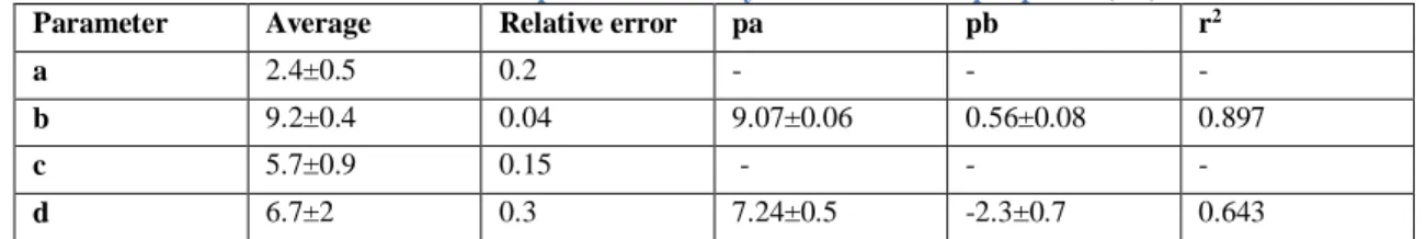
Figure 6 Same as Figure 4 for Conf c. Above: Monte Carlo simulated equatorial exosphere of O2 generated after O+ impacts in the configuration c of P2013. Below: density (O
2 after O+) obtained by 2D fit in the equatorial plane
Figure 7 Same as Figure 5. Parameters vs Lt for Conf c. Table 4 Results of parameters analysis case O+ Conf c
Parameter Value Rel. err.
p1 2.54(±0.1) 0.04 p2 9.60(±0.04) 0.004 p3 0.80(±0.06) 0.08 p4 5.0(±0.3) 0.06 p5 5.86(±0.2) 0.03 p6 -1.07(±0.06) 0.06
We can note that the density in this configuration is higher than the configuration a as well described by the parameter p2.
2.5 Cases Conf-b and Conf-d
In the case of O2 released after O+ impact when the Sun is toward Jupiter or anti
Jupiter (Figure 1), the density has a maximum at an angle between the subsolar point and the trailing direction. We need to use a new parameter to describe the shift angle. To be sure that a simple shift describes these configurations, we performed the 1D fit with eq. (1) and analysed the 4 free parameters of the density profiles versus Ln in the equatorial plane at radial distances R between 1.05 and 5 RE. The fits are shown in
Figure 8 and the parameters as a function of longitude are plotted in Figure 9 together with the fit with the function F = pa + pb cos(Ln+pc). The 4-parameters analyses are listed in Table 5 and Table 6.
Figure 8. As in Figure 2. 4-parameters fit of density profile Conf b (above) and Conf d (below) for all longitudes.
Figure 9. Conf b and Conf d parameters a, b, c and d vs Ln and weighted average intervals, fit function F=pa + pb cos(Ln+pc) is indicated by solid lines.
Table 5 Results of 4- parameters analysis for Conf b with function pa+pb*cos(Ln+pc)
Parameter Average Relative error
pa pb pc r2
a 1.9±0.4 0.21 - - - -
b 9.665±0.4 0.4 9.51±0.09 0.64±0.1 -37±10 0.857
Table 6 Results of 4- parameters analysis for Conf d with function pa+pb*cos(Ln+pc)
Parameter Average Relative error pa pb pc r2 a 2.0±0.5 0.25 - - - - b 9.65±0.4 0.4 9.5±0.1 -0.55±0.1 27±15 0.742 c 6.2±1 0.16 - - - - d 6.6±2 0.3 5.9±0.5 -0.6±0.7 20±60 0.713
Parameter b has again a clear trend versus Ln and an offset of -37° for Conf b, the same parameter for Conf d has a shifted trend (following the subsolar longitude S =
180°), in fact the pb sign is opposite for the two configurations with an offset of +27°. Parameter d seems to have a trend only for Conf d. The other parameters have no clear trend vs longitude as in the other configurations. For coherence with the previous functional form (5), we consider the function:
𝑙𝑜𝑔10𝜌 (𝑅, 𝛼𝑒𝑞, 𝛼𝑙𝑡) = (𝑝5 + 𝑝6cos (𝛼𝑒𝑞 − 𝑝7)cos (𝛼𝑙𝑡)) 𝑒—(𝑝4)(𝑅−1)−(𝑅−1)
𝑝1 + 𝑝2 +
𝑝3cos (𝛼𝑒𝑞 − 𝑝7)cos (𝛼𝑙𝑡) ( 6
where p7 is an angle function of the S, it is null at S=90° and 270° and
maximum/minimum at S=0° / 180°. For simplicity we consider the same p7
parameter for low and high altitudes. Finally, the functional forms of the parameters a, b, c, and d, as a function of the Sun-zenith angle, , are listed in Table 7.
Table 7 Results of a, b, c and d functional forms versus
Parameter function
a p1
b p2+p3*cos(-p7)
c p4
Figure 10 Same of Figure 4 for Conf b and Conf d. From above: P2013 Monte Carlo simulated equatorial exosphere of O2 generated after O+ impacts in Conf b; in Conf d; density obtained by 2D fit in the equatorial
plane for Conf b; for Conf d;.
Repeating the same procedure of Conf a and Conf c for these other configurations the resulting fits at the equatorial plane are shown in Figure 10. The resulting parameters versus Lt are plotted in Figure 11 and listed in Table 8
Figure 11 Same as Figure 5. Parameters vs Lt for Conf b above and Conf d below. Parameter p7 is expressed in radiants.
Table 8 Results of parameters analysis case O+ Conf b and Conf d
Parameter Value (Conf b) Rel. err. (Conf b) Value(Conf d) Rel. err. (Conf d)
p1 2.47(±0.1) 0.04 2.48(±0.2) 0.08 p2 9.33(±0.05) 0.005 9.32(±0.05) 0.005 p3 0.71(±0.06) 0.08 0.72(±0.03) 0.04 p4 5.29(±0.5) 0.09 5.27(±0.5) 0.09 p5 5.83(±0.2) 0.03 5.83(±0.08) 0.01 p6 -0.92(±0.1) 0.1 -0.91(±0.06) 0.07 p7 -25(±4) 0.2 31(±3) 0.1
2.6 Dependence by orbit phase
From the resulting fit parameters it is clear that some of them modulate along the Europa orbit around Jupiter while others are about constant.
We consider as constant parameters (values within the error in the four configurations) p1 and p4, which are the parameters describing the profile versus altitude.
We express the parameters p2, p3, p5, p6 and p7 as a function of orbit phase, that is, of the position of the Sun, S. Having only four points, we suggest a simple harmonic
function; hence, the functional forms of each parameters are expressed in Table 9. Finally a 4D analytical model is obtained.
Table 9. Functional form of the parameters
Parameter Functional forms Functions
p1 const 2.51
p2 p2(S=0)-(p2(S=270)-p2(S=90))/2*sin(S) 9.3-0.3*sin(S)
p3 p3(S=0)-(p3(S=270)-p3(S=90))/2*sin(S) 0.71-0.09*sin(S)
p4 const 5.2
p7 p7(S=0) *cos(S) -28*cos(S)
2.7 Corrections
To obtain the total O2 density at Europa, the obtained parameters must be corrected
for two reasons.
1) The O2 release yields used in P2013 need to be revised similarly to the updates in
Plainaki et al. (2015) following the argumentations described in Section 2.7.1.
2) This analysis has been performed by considering only the O+ ions impacting the icy surface. The contribution of different ions, mainly H+ and S+ must be added to this density profile according to the argumentations described in Section 2.7.2.
2.7.1 Yield revision
In P2013 an erroneous interpretation of the surface-binding energy parameter, U, included in the Famà et al. (2008) formula had been considered. In particular, while incorporating the Famà formula in the EGEON model, the experimentally derived value of U = 0.05 eV (Boring et al., 1984; Brown et al., 1984) was considered. However, such a consideration ignored the fact that the original lab data were fit in a formula that used the value of the water sublimation energy, U = 0.45eV, rather than the experimentally derived value. Therefore, the yield values, in the whole energy range and for all three species (H+, O+, S+), must be corrected by a factor c
1, equal to
0.05/0.45.
Moreover, while calculating the O2 release yield, within the EGEON model, only
normal ion incidence had been considered. Whereas, non-normal ion incidence can increase the surface release yield (e.g. Johnson, 1990), the existence of regolith regions can lower the yield (Cassidy et al., 2013). The two effects on the yield could cancel each other. By considering the case of a pure ice surface, we choose to correct our calculations for the O2 release yield by inserting an additional correction factor, c2, that represents the angle-averaged yield. This factor is equal to the average value
of cos-f(θ), with the incidence angle θ varying in the (0-70) degrees range (Wei et al., 2009). Therefore, for the incidence-angle correction factor, c2, we derive the
following values: O+ (m1=16 --> f=1.7): c
2=2
S+ (m1=32 --> f=1.8 ): c2=2
H+ (m1=1 --> F=1.3 ): c2=1.6
A third correction to the formula of the yield regarding the fractioning of the Famà et al., (2008) formula must be considered. P2013 fractioned the temperature-dependent part of the formula, Ydiss(T), in a stoichiomteric way, that is, 2-to-1 H2-to-O2
partitioning and, therefore, YO2=1/3 * Ydiss(T) However, the mass of these molecules
must be considered. This means that it is more correct to consider .
Finally, this yield a third correction factor to be applied which is c3=3/2.
In conclusion, the EGEON model of P2013 must be scaled by a factor of
c1*c2*c3=1/3, that is, a factor –log10(3) in function (6). This factor modifies only the
p2 parameter.
2.7.2 Other ions effects
This analysis has been performed by considering only the O+ impacting the icy
surface. The contribution of different ions, i.e.: H+ and S+ must be added to this
density profile. We can consider that H+ and S+ have similar impacting distributions,
Y
Oso that the obtained released densities can be simply added to that obtained from O+ impact to have the total O2density.
As summarized in Table 1 of P2013 the ratios of the density due to H+ and to S+ to
the density due to O+are a factor 0.5 and 0.008, respectively.
To obtain the total O2density, the density after O+ impact must be multiplied by a
factor c4= 1.508, that is, a factor log10(1.508) in function (6). Also this factor modifies
the parameter p2, that finally becomes p2= p2-log10(3)+log10(1.508)=p2-0.3.
3 Discussion
The analytical model of the O2 distribution resulting from the EGEON model is a
7-parameters Chamberlain function of Europa centric distance R, angle from the subsolar point in the equatorial plane eq and Lt as shown in eq (5). This model
describes the O2 profiles in the altitudes range from 1.05 to 5 RE according to the
range of the source model P2013, nevertheless, the profiles could be extrapolated down to 1 RE as a first approximation. The EGEON model assumes non-collisional
regimes. Possible close-to-surface additional effects are expected only at subsolar point where higher temperatures, up to 132 K, increase the H2O sublimation rate
producing a vapor pressure of the order of 1012 Pa, hence a non-collisional condition could occur (Smyth and Marconi, 2006; Plainaki et al., 2010). Only in that region the close-to-surface density profile could significantly differ from the extrapolated one. The function trend versus altitude (parameters a of Eq. 1) ) is not -dependent or Configuration dependent at high altitudes. In fact, the density profile versus altitude is driven by the energy distribution of the emitted particles and at high altitudes only the more energetic particles released after radiolysis are present. The emitted O2 energy
distribution assumed in EGEON is a fit to an equivalent laboratory measurement (Johnson et al., 1982; Brown et al., 1984) used also in previous analyses:
( 7
where U0=0.015eV (Shematovich et al., 2005), an is the normalization factor and Ee is
the energy of the ejected O2 molecules.
The parameters b and d are dependent on , as expected, since the released O2 is
dependent on the impacting ion flux and on yield of the release (number of particles released by single ion). The yield of the radiolytic release is dependent on temperature and on impacting energy (Famà et al., 2008).
The surface temperature map considered in P2013 was the one given in Spencer et al. (1999), based on Galileo mission data. In particular, the temperature map was assumed as 40 + 50cos(Lt)1/4 + 40cos() K in the dayside, and 40 + 50 cos(Lt)1/4 K in the nightside (Cassidy et al., 2007). A preferential O2 ejection from the trailing
hemisphere was considered in EGEON (see Eq. (4) in Plainaki et al. 2012). This may occur due to preferential ion (Pospieszalska and Johnson, 1989) or electron (Paranicas et al., 2001) irradiation. As evidenced in P2013 the temperature effect is predominant with respect to the impacting flux effect, but the release is higher when the trailing hemisphere coincides with the illuminated side, as well described by parameter p2. By fitting the vertical profile with the barometric profile, the exospheric temperature can be derived: 𝜌 = 𝜌1exp (−(𝑅 − 𝑅1)
𝐻
⁄ ), where 1 is the density at R1 that is the
minimum altitude, H is the scale height defined as 𝐻 =𝑘𝐵𝑇
𝑚𝑂2𝐺𝑀𝐸
𝑅12
⁄ , where kB is
constant, ME is the Europa’s mass. From these relations the temperature, T, can be
easily derived.
As evidenced before, the obtained density profiles evidence that there are two exosphere scale heights, thus two temperatures describing the neutral population at low and high altitudes in the Europa’s environment.
We performed two separate fits of the exosphere density profiles: one corresponding to region 1.05 < R < 1.5 RE (low altitudes) and one to region 2 < R < 5 RE (high
altitudes). In Figure 12 the derived profiles at low and high altitudes are shown in the case of Conf a for the trailing and the leading hemisphere profiles.
It is clear that both the densities and the temperatures are higher in the illuminated side. The temperature at low altitudes in the illuminated side (Til= 270 K) is higher
than in the dark side (Tdl= 210 K), with a relative variation about 25%. This result can
be interpreted as follows: the low-altitude O2 exosphere is the result of a
density-weighted combination of both the surface-thermalized component (the surface temperature is about 130 K in the subsolar point) and the more energetic radiolytically-released population. The low temperature at low altitudes - dark side is the indication of a major weight of the population thermalized at lower temperatures, with respect to the illuminated side. The proposed scenario includes a first release after radiolysis with a yield proportional to ion flux and temperature, then the molecules start bouncing and to be thermalized with the surface. The lifetime of the thermalized component is driven by the loss via electron impact dissociation (considered symmetric and of the order of 107 s in the EGEON model), longer than the ballistic flight time (Plainaki et al. 2012), so that, the intense atmosphere around the moon is, in fact, generated by this thermalized population, as mentioned in the introduction.
The temperature for the higher altitudes is less variable, between 2170 and 2200 K; in fact, the relative variation is less than 2%. This uniformity was expected since the higher altitudes profile is generated by the temperature-independent energy distribution of radiolysis release (equation 7).
Figure 12 Examples of equatorial vertical profile for Conf a and derivation of temperature at low and high altitudes.
The two temperatures can be easily derived for each longitude and configuration (Figure 13). Tl/Tl is about 30% and Th/Th about 2%. The average scale height at
related to the parameters in Table 9. In fact, we can approximate the analytical model 6) at low altitudes as:
𝜌𝑙 (𝑅 < 1.5) ≈ 10𝑝2+𝑝5exp (− ln(10) (p5 p4 + 1
𝑝1) (R − 1)) 𝜌ℎ (𝑅 > 2) ≈ 10𝑝2+𝑝5exp (−𝑝4)exp (− ln(10) ( 1
𝑝1) (R − 1))
The analytical scale heights at R=1RE and at R=2RE are, then, Hl=0.014 RE = 20 km
(corresponding to 124 K) and Hl=1.1 RE = 1700 km (2400 K), respectively, in
agreement with the fitted-derived values.
Figure 13 Temperatures obtained at different longitudes for low (right) and high (left) altitudes for the four configurations.
We note that in the lower region (< 1.5 RE) the average scale heights estimated with
our tool are in good agreement with the near-surface scale heights estimated in other studies. For example, Sittler et al. (2013), using the model by Amsif et al. (1997) and the parameters in Cassidy et al. (2007) estimated an O2 scale height that is increasing
with altitude being equal to 20 km near the surface and 32 km at the altitude of about 600 km.
4 Conclusions
A 3D analytical model of Europa’s O2 exosphere along the orbit around Jupiter
(which finally provides the fourth dimension of the equation) has been obtained with a simple functional form described by equation (6). The final parameters of the total molecular oxygen density distribution are summarized in Table 10.
Table 10 Analytical model parameters for total O2 density
As mentioned in the introduction, other molecular components like H and H O are Parameter Functions p1 2.51(±0.4) p2 9.0-0.3*sin(S) p3 0.71-0.09*sin(S) p4 5.2 p5 5.825-0.045*sin(S) p6 -0.92+0.155*sin(S) p7 -28*cos(S)
could be still a relevant fraction at higher distances. This model is intended to be the basic reference for the description of this O2 component. In the future, we aim to
develop further analytical models, with similar procedures, to describe also the other major components. This analytical model is a useful and user-friendly tool able to describe the bulk and especially the high altitude exospheric profiles and the expected asymmetries.
The model is able to reproduce the asymmetries in the O2 distributions and their
modulations due to the configurations among Europa, Jupiter and the Sun. Furthermore, the parameterization of the O2 density distribution with parameters able
to describe separately the different altitude ranges and the asymmetries in longitude and in orbit phase is an elegant way to quantify the density profile properties.
The analytical model permits to evidence and quantify the two-temperature components of the exosphere, and the longitude asymmetries of the low altitude temperatures.
This model could be optimized by including secondary effects like loss by dissociation by UV photons or charge-exchange with ambient plasma. It could be used as a tool in many possible applications in the context of a) theoretical studies related to the plasma-neutrals interactions at Europa; b) planning of either space mission observations or observations with ground and/or space telescopes; c) analysis of in situ and/or remote sensing data (e.g. obtained with HST and other telescopes). Here, we just highlight few examples.
Through this tool, input for plasma circulation models can be provided and feedback for the evaluation of plasma sources (e.g. electron-impact ionization) and losses (e.g. charge-exchange) in the near-Europa space environment can be obtained
During preparation for future missions to Europa, this tool can be used in ENA simulations; once future ENA measurements are available, the tool can be used while performing plasma deconvolution procedures.
The tool can be used for the interpretation and analysis of the remote sensing observations, helping in the identification of sporadic phenomena.
Through this tool the bulk exosphere population can be obtained; this information can be used as an input for minor exospheric species simulations. The atmospheric physics of the Galilean moons of Jupiter, and in particular of Europa, is one of the major interests of the international scientific community. The recent observations with HST of Europa's O2 environment (McGrath et al., 2004; Saur
et al., 2011; Roth et al., 2014) and their potential implication on the nature of the moon's inner ocean, as well as subsequent debates on the interpretation of in situ and remote observations (Shemansky et al., 2014), opened a new chapter in the study of Europa's O2 environment. In this context, the accurate characterization of the moon's
exospheric O2 background is a mandatory prerequisite. The analytical model
presented in the current paper aims at providing the necessary link between observable quantities and physical processes. In particular, the scale heights for different components could be obtained during a mission to the icy moons. A comparison with the presently estimated quantities will directly provide information on the source process. Finally, the availability to the science community of the analytical model of Europa's O2 exosphere may be of significant interest in view of
Discussions in this paper have been partially performed in the context of the activities of the ISSI International Team #322, http://www.issibern.ch/teams/exospherejuice/. This work is partially supported by the ASI contract no. I/081/09/0.
5 References
Amsif 1997Boring, J.W., Garrett, J.W., Cummings, T.A., Johnson, R.E., Brown, W.L., 1984. Sputtering of solid SO2. Nucl. Instrum. Methods B 1, 321–326.
Brown, W.L. et al., 1984. Electronic sputtering of low temperature molecular solids. Nucl. Instrum. Methods Phys. Res. B 1, 307–314.
Cassidy, T.A., Johnson, R.E., McGrath, M.A., Wong, M.C., Cooper, J.F., 2007. The spatial morphology of Europa’s near-surface O2 atmosphere. Icarus 191, 755–764.
Cassidy et al., 2010, Radiolysis and Photolysis of Icy Satellite Surfaces: Experiments and Theory, Space Science Reviews, 153, Issue 1-4, 299-315.
Cassidy, T.A, et al., 2013. Magnetospheric ion sputtering and water ice grain size at Europa. Planetary and Space Science 77, 64–73.
Chamberlain, J. W., 1963, Planetary coronae and atmospheric evaporation, Planet. SpaceSci., 11, 901.
Cooper et al., 2001, Energetic ion and electron irradiation of the icy Galilean Satellites, Icarus 149, 133-159.
Famà et al. 2008, Sputtering of water ice by low energy ions, Surface Sci. 602, 156 Johnson et al., 1982, Planetary applications of ion-induced erosion of condensed-gas
frost, Nucl. Instrum. Methods, 198, 147
Johnson, R.E., 1990. Energetic charged-particle interactions with atmospheres and surfaces. Springer-Verlag eds. ISBN 3-540-51908-4 Berlin Heidelberg New York Johnson et al., 2004. Radiation Effects on the Surface of the Galilean Satellites, in:
Jupiter-The Planet, Satellites and Magnetosphere, Ed. F. Bagenal, T. Dowling, and W.B. McKinnon, Cambridge University, Cambridge. Chapter 20, 485-512
Johnson, R.E., et al., 2009. Composition and Detection of Europa’s Sputter-Induced Atmosphere. In: Pappalardo, R.T., McKinnon, W.B., Khurana, K.K. (Eds.), Europa. University of Arizona Press, Tucson.
Leblanc, F., Johnson, R.E., Brown, M.E., 2002. Europa’s sodium atmosphere: An ocean source? Icarus 159, 132–144.
McGrath et al., 2004; Satellite atmospheres, In: Jupiter. The planet, satellites and magnetosphere. Ed. F. Bagenal, T. E. Dowling, W.B. McKinnon, Cambridge University Press., Vol. 1, 457 – 483
Paranicas, C., Carlson, R.W., Johnson, R.E., 2001. Electron bombardment of Europa. Geophysical Research Letters 28, 673–676.
Paranicas et al., 2002, The ion environment near Europa and its role in surface energetics, Geophys. Res. Letters, 29 (5), 1074
Plainaki et al., 2010, Neutral particle release from Europa’s surface, Icarus, 210, 385– 395.
Plainaki et al., 2012, The role of sputtering and radiolysis in the generation of Europa exosphere, Icarus, 218 (2), 956–966.
P2013 Plainaki et al., 2013, Exospheric O2densities at Europa during different orbital
phases, Planetary and Space Science, 88, 42-52.
Plainaki, et al., 2015. The H2O and O2 exospheres of Ganymede: the result of a
Pospieszalska, M.K., Johnson, R.E., 1989. Magnetospheric ion bombardment profiles of satellites—Europa and Dione. Icarus 78, 1–13.
Roth et al. Transient water vapor at Europa’s south pole. Science, 343, 171, 2014 Saur, J. et al., 1998 Interaction of the Jovian magnetosphere with Europa: Constraints
on the neutral atmosphere. J. Geophys. Res., 103.
Saur et al. 2011, Hubble Space Telescope/Advanced Camera for Surveys Observations of Europa's Atmospheric Ultraviolet Emission at Eastern Elongation, Astroph. J., 738, 2, article id. 153.
Shemansky, D. E. et al., 2014 Understanding of the Europa atmosphere and limits on geophysical activity. Astrop. J., 797, 84.
Shematovich et al., 2005, Surface-bounded atmosphere of Europa. Icarus 173, 480-498.
Sittler 2013
Smyth and Marconi, 2006. Europa’s atmosphere, gas tori, and magnetospheric implications. Icarus 181, 510–526.
Spencer et al. (1999)
Wei et al., 2009. Influence of surface morphology on sputtering yields. J. Phys. D: Appl. Phys. 42 (2009) 165304 (6pp) doi:10.1088/0022-3727/42/16/165304